Precise Control of Both Dispersity and Molecular Weight Distribution Shape by Polymer Blending

Abstract

The breadth and the shape of molecular weight distributions can significantly influence fundamental polymer properties that are critical for various applications. However, current approaches require the extensive synthesis of multiple polymers, are limited in dispersity precision and are typically incapable of simultaneously controlling both the dispersity and the shape of molecular weight distributions. Here we report a simplified approach, whereby on mixing two polymers (one of high Đ and one of low Đ), any intermediate dispersity value can be obtained (e.g. from 1.08 to 1.84). Unrivalled precision is achieved, with dispersity values obtained to even the nearest 0.01 (e.g. 1.37→1.38→1.39→1.40→1.41→1.42→1.43→1.44→1.45), while maintaining fairly monomodal molecular weight distributions. This approach was also employed to control the shape of molecular weight distributions and to obtain diblock copolymers with high dispersity accuracy. The straightforward nature of our methodology alongside its compatibility with a wide range of polymerisation protocols (e.g. ATRP, RAFT), significantly expands the toolbox of tailored polymeric materials and makes them accessible to all researchers.

Tuning dispersity and molecular weight distribution shape significantly impacts polymer properties. Herein, we report a straight‐forward approach, wherein blending just two polymers allows for unrivalled precision in tuning molecular weight distributions.

Introduction

The term dispersity (Đ) is a measure of the spread of different molecular weight species within a polymeric material and is quantified by the ratio of the weight average (M _w) and number average molecular weights (M _n).[¹, ²] Both molecular weight distribution (MWD) shape and dispersity can significantly impact polymer properties including their overall performance, processability, self‐assembly and rheological behaviour.[³, ⁴, ⁵, ⁶, ⁷, ⁸, ⁹] Although low dispersity polymers (Đ<1.20) were initially the preferred target for polymer chemists,[¹⁰, ¹¹, ¹²] it has recently been demonstrated that moderate (Đ=1.20–1.50) and high dispersity (Đ>1.50) materials are equally desirable and exhibit complementary properties and characteristics.[⁷, ¹³, ¹⁴, ¹⁵, ¹⁶] This has resulted in the development of various chemistry and engineering methods to target different dispersity values and to tailor MWD shapes.[³, ⁸, ¹⁷, ¹⁸, ¹⁹, ²⁰, ²¹, ²²]

Polymer blending is the most famous and widely used approach owing to its great simplicity. Polymers consisting of different molecular weights are mixed in predetermined ratios to obtain the desired MWD.[²³, ²⁴, ²⁵, ²⁶] These polymers usually possess comparable dispersity values; they are either all of high dispersity when synthesised through free radical polymerisation or all of relatively low dispersity when controlled polymerisation strategies are employed.[²⁷, ²⁸, ²⁹, ³⁰] The main drawback of this strategy is that a large number of polymers (typically >10) have to be synthesised and rigorously purified prior to blending, thus making the process tedious and time‐consuming.[²⁶, ³¹] Another limitation is that common blending strategies either result in a narrow dispersity window (e.g. when discrete oligomers are mixed) or yield bimodal and multimodal MWDs.[¹⁸, ²⁹, ³², ³³]

To target more continuous distributions with much wider dispersity ranges, a number of alternative strategies have recently emerged. For instance, Fors and co‐workers reported an elegant strategy, which allows for the deterministic control of MWDs by regulating the rate of initiator addition in controlled polymerisation methods such as nitroxide mediated polymerisation and anionic polymerisation.[⁵, ⁶, ¹⁷, ³⁴, ³⁵, ³⁶] Although this method enables full control over the shape of MWDs, it is less powerful to yield fully monomodal, continuous and symmetric SEC traces as it is often accompanied by low molecular weight tailing due to the delayed initiation of some polymer chains. In a different approach the groups of Boyer, Junkers, Frey, Leibfarth and Guironnet have developed flow methods to alter MWDs for a range of polymerisation methodologies.[¹⁸, ¹⁹, ²⁰, ²², ²⁴, ³⁷, ³⁸, ³⁹, ⁴⁰] Such methods require the use of syringe pumps and may also employ mathematical models and software. Importantly, for all the aforementioned strategies an individual polymerisation must be performed for each MWD shape or dispersity required. For example, if 20 different dispersity values are needed, 20 individual polymers have to be synthesised and purified.

In addition, strategies that directly manipulate the chemistry of polymerisation equilibriums to control chain growth have been exploited. By either changing the catalyst concentration in atom transfer radical polymerisation (ATRP), mixing chain transfer agents of different activity in reversible addition fragmentation chain transfer (RAFT) polymerisation or through the reversible photo‐isomerisation of initiators in cationic polymerisation, a range of dispersities values can be produced while preserving high‐end group fidelity.[⁴¹, ⁴², ⁴³, ⁴⁴, ⁴⁵, ⁴⁶, ⁴⁷, ⁴⁸] Although these methods can tune the dispersity, they do not allow for any control over the shape of MWDs. There are others caveats to these processes too. Like with all the flow and initiation regulation methods, chemistry approaches also demand the synthesis of a new polymer for each targeted dispersity, which may lead to extensive synthesis cycles. This issue is further amplified when a consistent molecular weight is needed for all targeted dispersity values as many chemistry methods suffer from a loss of initiator efficiency.[⁴³, ⁴⁴] An additional disadvantage is that the accuracy in synthesising a polymer of a chosen dispersity is commonly limited to the nearest 0.1–0.2, which may also affect the reproducibility of the developed approaches. Other methods involve the addition of termination agents or co‐monomers to control polymer dispersity, thus leading to partially terminated chains and adulterated polymer chains, respectively.[⁴⁹, ⁵⁰, ⁵¹]

To overcome the aforementioned limitations, we sought to develop a new method where both the shape of MWDs and dispersity could be efficiently and precisely controlled by simply mixing only 2 polymers (Figure 1). To achieve this, low (Đ≈1.08) and high dispersity (Đ≈1.84) polymers of comparable M _p were first synthesised. By subsequently blending these two polymers in different ratios, a wide range of monomodal molecular weight distributions could be obtained. Importantly, our method can, for the first time, accurately and precisely prepare polymers with dispersity values within 0.01 of those targeted. The resulting polymers also possess very high end‐group fidelity, as exemplified by chain extensions forming dispersity controlled diblock copolymers. Furthermore, our approach can simultaneously control both the shape of the molecular weight distribution and the dispersity, allowing predictable access to a wide range of systematically skewed materials.

Figure 1.

Previous approaches and our current approach in tuning the dispersity.

Results and Discussion

Our first target was to synthesise two polymers with the same peak molecular weight and significantly different dispersity values. We selected photoATRP as an exemplary method owing to its simplicity and potential to access dispersity extremes, (e.g. both low and high values) while also maintaining very high end‐group fidelity (Scheme S1).^[43] With a high catalyst concentration (2 % w.r.t initiator) low dispersity poly(methyl acrylate) (PMA) was obtained with a dispersity of 1.08, (P1, M _n=24900, M _p=25800, Figures S1a & S2a) while with a low catalyst concentration (0.05 % w.r.t initiator) high dispersity PMA was prepared with a dispersity of 1.84 (P2, M _n=15200, M _p=25,400, Figures S1b & S2b). These two polymers were subsequently purified, by extraction to remove catalyst and solvent, and then dialysis to remove any unreacted monomer (and initiator in the high dispersity case), before being dried to constant mass under vacuum.

We next simulated the process of mixing these two polymers. In size exclusion chromatography (SEC), log molecular weight is typically plotted against intensity (dw/dlogM), with the area under the curve directly proportional to the weight concentration of the polymer (Figure S3).^[52] Thus, low dispersity polymers have fewer different molecular weight species but each has a much higher intensity compared to those of a high dispersity sample. We simulated mixing the low and high dispersity polymers, by running SEC of these samples, normalising their areas and then adding them together in different ratios. We then calculated the dispersity of these mixtures to investigate how dispersity evolved with composition (Table S1, Figures 2 a & S4). Importantly, the overall dispersity of the blended mixture increased linearly with the percentage increase of the high dispersity polymer. For example, a 1:1 mixture by weight, yielded an intermediate dispersity value of 1.46 (the middle value between 1.08 and 1.84, Table S1 Entry 6). This allowed us to generate the following equation, Đ _mix=Ð _P1 + Wt%_P2(Ð _P2−Ð _P1), which can be used to predict the dispersity value of any subsequent mixture, where the overall dispersity of the blended mixture (Đ _mix) is equal to the dispersity value of the first polymer (Ð _P1) plus the weight percentage of the second polymer (Wt%_P2) multiplied by the difference in dispersity of the two polymers (Ð _P2−Ð _P1). For example, a 1:4 ratio of low to high dispersity polymer, gives a predicted Đ _mix of 1.69 (Đ _mix=1.08 + 0.8(1.84−1.08). Thus, for every additional 10 % of the high dispersity polymer, the dispersity incrementally increased by 0.07 or 0.08 (Figure 2 a).

Figure 2.

Simulation and real SEC data for mixing one low dispersity and one high dispersity PMA. a) and b) illustrate the simulated SEC traces and predicted dispersity values for different polymer compositions and c) and d) illustrate the obtained SEC data and dispersity values for mixtures of these two polymers.

Having successfully simulated the blending process, we wanted to see if in reality mixing these polymers could provide such precision. As SEC samples are typically measured at ≈1 mg mL⁻¹ concentrations, we prepared a stock solution of each polymer thus avoiding any error from weighing small amounts of polymers. On mixing the two polymers in a 1:1 ratio, pleasingly the predicted dispersity of 1.46 was obtained to within an error of 0.01 (Ð _50:50=1.45), illustrating how accurately dispersity values can be targeted with our method (Table S2 Entry 6, Figures 2 b & S5). Similarly, when the polymers were mixed in a ratio of 1:4, the predicted dispersity of 1.69 was obtained to within an error of 0.01 (Ð _20:80=1.68) further exemplifying the precision of this system (Table S2 Entry 3, Figures 2 c,d). We next ran a sequence of SEC measurements, in which the amount of low and high dispersity polymer were carefully varied (100:0, 90:10, 80:20, 70:30, 60:40, etc.). Again, excellent accuracy was achieved for every measurement, with consistent changes in dispersity as the ratio of the two polymers was changed (i.e. Ð _100:0=1.08, Ð _90:10=1.15, Ð _80:20=1.22, Ð _70:30=1.30, Ð _60:40=1.37, Ð _50:50=1.45, Ð _40:60=1.53, Ð _30:70=1.60, Ð _20:80=1.68, Ð _10:90=1.76, Ð _0:100=1.84, Table S2, Figures 2 c,d & S5). Together this data illustrates that by blending just two polymers, numerous different dispersity values can be precisely obtained. The simplicity of this approach contrasts previous methods, where to obtain these distributions either 11 different polymers would have to be prepared and purified, or numerous low dispersity materials would need to be synthesised, purified and then blended.^[43] Furthermore, the correlation between the predicted dispersity and that of the obtained polymer is unparalleled by any other method. Another important advantage of our approach is the high reproducibility, with dispersity values consistently obtained to within 0.01 (Table S3). Therefore, as long as the first two polymers are successfully synthesised, any intermediate value can be obtained with high accuracy. This is in contrast to chemistry methods where targeting a precise value (e.g. 1.45) may require several synthetic iterations.^[43]

Next, we were interested in investigating whether even greater precision could be achieved with this system. No reported method can simply target individual dispersity values and obtain them to the nearest 0.01, so we therefore selected two consecutive ratios from the previous experiment (Ð _60:40=1.37 and Ð _50:50=1.45) and targeted each dispersity value in between. First a mixture of 45 % low dispersity polymer and 55 % high dispersity polymer was prepared and, pleasingly, an intermediate dispersity of 1.41 was obtained (Table 1 Entry 5, Figures 3 & S6). Next six further ratios were prepared with incremental changes in composition (3 compositions with between 40 & 45 % of P2 and 3 compositions with between 45 & 50 % of P2). Pleasingly, every individual polymer dispersity could be obtained with Ð _58.7:41.3=1.38, Ð _57.5:42.5=1.39, Ð _56.2:43.8=1.40, Ð _55:45=1.41, Ð _53.8:46.2=1.42, Ð _52.5:47.5=1.43 and Ð _51.2:48.8=1.44 (Table, Figures 3 & S6). It is very impressive that such level of accuracy could be obtained, which highlights the robustness of our method. It is also important to note that the analytical techniques utilised (e.g. balance and SEC) are sufficiently accurate to reveal this level of precision. Taken altogether, this approach is not only incredibly simple to perform, but has precision unmatched by any other chemistry, engineering or blending method.

Table 1.

SEC data for the precision mixing of high and low dispersity PMA illustrating incremental increases in dispersity as the amount of high dispersity polymer was increased.^[a]

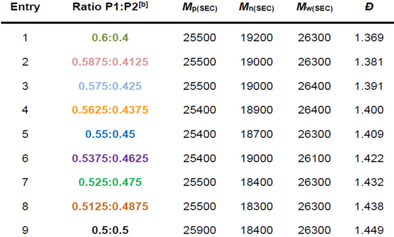
[a] Molecular weight and dispersity values were determined by SEC. [b] P1:P2 is the ratio of low dispersity to high dispersity polymer. Colours match the SEC traces in Figure 3.

Figure 3.

Overlapping SEC traces illustrating 9 consecutive dispersity value polymers (Đ=1.37→1.45) formed by mixing high and low dispersity PMA. Inset are two expanded in segments of the spectrum.

One of the great benefits of controlled radical polymerisation is that the polymers produced can possess high end‐group fidelity which allows for the generation of block copolymers. In turn, block copolymers are used in a wide range of applications[⁵³, ⁵⁴] We therefore investigated whether we could incorporate our high level of precision into diblock copolymers by chain extending macroinitiator (MI) mixtures. Our low dispersity (M _n=24,900, M _p=25800, Ð=1.08) and high dispersity polymers (M _n=15200, M _p=25,400, Ð=1.84) were mixed in ratios of 3:1 and 1:3 so to obtain macroinitiators with selected dispersity values of 1.25 and 1.64 (Table S4 & Figure 4). With these mixtures, chain extensions were performed with photoATRP, using a high concentration of catalyst, so to generate low dispersity diblocks and allow for clear shifts in the MWDs. Successful chain extension were evidenced by high polymerisation conversions, large shifts in the molecular weight distributions and decreases in dispersity, with final dispersities of 1.12 (Ð _MI=1.25, Table S4 & Figure 4 a) and 1.14 (Ð _MI=1.64, Table S4 & Figure 4 b). Together this demonstrates that the dispersity of the first block can simply be selected and prepared, before subsequent chain extension is performed. This avoids the time‐consuming optimisation of previous approaches, whereby many polymers would need to be blended or each individual dispersity value diblock copolymer would need to be optimised and prepared.

Figure 4.

SEC analysis for the chain extension of macroinitiators formed by mixing one low and one high dispersity PMA, in a ratio of a) 3:1 and b) 1:3.

In addition to controlling the MWD breadth and associated dispersity value, we also investigated whether our approach could precisely tune the shape of the MWD. Methods to control the shape though, are much more limited and often are not able to simultaneously control both the shape and the dispersity.[³, ⁴] First we prepared a low dispersity polymer with the same number average molecular weight (M_n=15,000, Ð=1.09) as our initially employed high dispersity polymer and then we mixed these two polymers in different ratios. Pleasingly, our simulation illustrated that the shape of the distribution could be systematically changed, while simultaneous controlling the dispersity value (Table S5, Figures S8–10). In fact, a linear relationship between the composition of the mixture and its overall dispersity was again observed, with the trend‐line Đ=Ð _P1+W%_P2(Ð _P2−Ð _P1).

We therefore mixed the polymers in a range of ratios (100:0, 90:10, 80:20, 70:30 etc.), generating a gradual skew to high molecular weight and an incremental increase in dispersity (i.e. Ð _100:0=1.09, Ð _90:10=1.14, Ð _80:20=1.24, Ð _70:30=1.30, Ð _60:40=1.38, Ð _50:50=1.44, Ð _40:60=1.54, Ð _30:70=1.61, Ð _20:80=1.68, Ð _10:90=1.76, Ð _0:100=1.84, Table S6, Figures 5 a & S11–13). Next, we wanted to skew the distribution in the opposite direction, so to gradually increase the amount of low molecular weight species. We therefore simulated mixing the high dispersity polymer with different molecular weight low dispersity polymers (M _n =20,000–60,000, Ð=1.08), so to obtain the mirrored molecular weight distribution shape. Based on the difference in log M _p values for the high and low dispersity M_n alignment, we ascertained that the molecular weight required was around 35,000 (Table S7, Figure S14). This was again synthesised by photoATRP with a final M _n of 35500 and a dispersity of 1.08 (Figure S15). Pleasingly, mixing this polymer with our high dispersity polymer, the molecular weight distribution was systematically skewed to lower molecular weight, with observed trace intensities directly corresponding to those previously skewed in the opposite direction (Table S8, Figures S16–18). We should note that, unlike the previous examples, there isn't a linear evolution in dispersity with the mixing ratio (i.e. Ð _100:0=1.07, Ð _90:10=1.18, Ð _80:20=1.29, Ð _70:30=1.39, Ð _60:40=1.48, Ð _50:50=1.57, Ð _40:60=1.66, Ð _30:70=1.71, Ð _20:80=1.77, Ð _10:90=1.82, Ð _0:100=1.84, Table S9, Figures 5 b & S19). This is due to a greater difference in molecular weights of the two polymers resulting in slightly higher dispersity values. All in all, this data shows that our simple method is compatible with shape control and by changing the molecular weight of the low dispersity polymers, desired distributions can be designed and tailored.

Figure 5.

SEC data illustrating molecular weight distribution shape control utilising our blending process, with a) gradual skewing of the distribution to high molecular weight and b) gradual skewing of the distribution to low molecular weight.

Finally, we wanted to apply our methodology to another polymerisation type and monomer class, so we selected RAFT as an alternative polymerisation technique. We first used thermal RAFT and then photo‐induced electron/energy transfer (PET) RAFT to prepare both high and low dispersity poly(methyl methacrylate) (PMMA).[⁴⁶, ⁴⁷, ⁵⁵] 4‐Cyano‐4‐(phenylcarbonothioylthio)pentanoic acid (CTA1) and 2‐cyanobutan‐2‐yl 4‐chloro‐3,5‐dimethyl‐1H‐pyrazole‐1‐carbodithioate (CTA2) were selected as the high and low activity CTAs, respectively (Figure S20). With thermal RAFT, PMMA was obtained with dispersities of 1.13 (M _n=27200, M _p=31100, Figure S21a) and 1.69 (M _n=20400, M _p=31200, Figure S21b), respectively. These polymers were purified by dialysis in acetone, before being dried to constant mass under vacuum. Next the polymers were mixed in 11 different ratios (100:0, 90:10, 80:20, 70:30 etc.). Again, the dispersity increased linearly with the addition of high dispersity polymer illustrating predictable and precise values (i.e. Ð _100:0=1.13, Ð _90:10=1.19, Ð _80:20=1.25, Ð _70:30=1.30, Ð _60:40=1.36, Ð _50:50=1.42, Ð _40:60=1.47, Ð _30:70=1.53, Ð _20:80=1.58, Ð _10:90=1.64, Ð _0:100=1.69, Tables S10–11, Figures S22–25). With PET RAFT, PMMA was obtained with final dispersities of 1.22 (M _n=21200, M _p=27300, Figure S26a) and 1.59 (M _n=18100, M _p=26500, Figure S26b). These polymers were purified by passing through a short column of alumina prior to dialysis and drying. Similarly, on mixing, the dispersity increased linearly with the addition of high dispersity polymer (i.e. Ð _100:0=1.22, Ð _90:10=1.25, Ð _80:20=1.29, Ð _70:30=1.32, Ð _60:40=1.36, Ð _50:50=1.39, Ð _40:60=1.43, Ð _30:70=1.47, Ð _20:80=1.50, Ð _10:90=1.55, Ð _0:100=1.59, Tables S12–13, Figures S27–30). This verifies that our system is compatible with a wide range of reported methods whereby both high and low dispersity polymers can be obtained, allowing for facile access to all intermediate values.

Conclusion

To summarise, we report a straight‐forward and predictable blending method which allows for a wide range of dispersities to be obtained. By simply mixing two polymers in precise ratios, all intermediate dispersity values can be accessed with accuracy illustrated to the nearest 0.01. Not only does this approach afford unparalleled precision in dispersity control, it can be applied to the synthesis of both homo and block copolymers and is compatible with a wide range of polymerisation protocols. In addition, the shape of the molecular weight distributions can also be efficiently controlled. The simplicity of this method will allow not only chemists but also scientists from different fields to precisely tune molecular weight distributions on demand.

Conflict of interest

The authors declare no conflict of interest.

Supporting information

As a service to our authors and readers, this journal provides supporting information supplied by the authors. Such materials are peer reviewed and may be re‐organized for online delivery, but are not copy‐edited or typeset. Technical support issues arising from supporting information (other than missing files) should be addressed to the authors.

Supporting Information

Supporting Information

R. Whitfield, N. P. Truong, A. Anastasaki, Angew. Chem. Int. Ed. 2021, 60, 19383.

References

- 1.Stepto R. F., Pure Appl. Chem. 2009, 81, 351–353. [Google Scholar]
- 2.See Ref. [1].
- 3.Whitfield R., Truong N. P., Messmer D., Parkatzidis K., Rolland M., Anastasaki A., Chem. Sci. 2019, 10, 8724–8734. [DOI] [PMC free article] [PubMed] [Google Scholar]
- 4.Gentekos D. T., Sifri R. J., Fors B. P., Nat. Rev. Mater. 2019, 4, 761–774. [Google Scholar]
- 5.Rosenbloom S. I., Fors B. P., Macromolecules 2020, 53, 7479–7486. [Google Scholar]
- 6.Nadgorny M., Gentekos D. T., Xiao Z., Singleton S. P., Fors B. P., Connal L. A., Macromol. Rapid Commun. 2017, 38, 1700352. [DOI] [PubMed] [Google Scholar]
- 7.Gentekos D. T., Jia J., Tirado E. S., Barteau K. P., Smilgies D.-M., R. A.DiStasio, Jr. , Fors B. P., J. Am. Chem. Soc. 2018, 140, 4639–4648. [DOI] [PubMed] [Google Scholar]
- 8.Sifri R. J., Padilla-Vélez O., Coates G. W., Fors B. P., J. Am. Chem. Soc. 2020, 142, 1443–1448. [DOI] [PubMed] [Google Scholar]
- 9.Chatzigiannakis E., Vermant J., Soft Matter 2021, 17, 4790–4803. [DOI] [PubMed] [Google Scholar]
- 10.Perrier S. B., Macromolecules 2017, 50, 7433–7447. [Google Scholar]
- 11.Matyjaszewski K., Adv. Mater. 2018, 30, 1706441. [DOI] [PubMed] [Google Scholar]
- 12.Parkatzidis K., Wang H. S., Truong N. P., Anastasaki A., Chem 2020, 6, 1575–1588. [Google Scholar]
- 13.Yadav V., Jaimes-Lizcano Y. A., Dewangan N. K., Park N., Li T.-H., Robertson M. L., Conrad J. C., ACS Appl. Mater. Interfaces 2017, 9, 44900–44910. [DOI] [PubMed] [Google Scholar]
- 14.Junkers T., Macromol. Chem. Phys. 2020, 221, 2000234. [Google Scholar]
- 15.Li T.-H., Yadav V., Conrad J. C., Robertson M. L., ACS Macro Lett. 2021, 10, 518–524. [DOI] [PubMed] [Google Scholar]
- 16.Wang C.-G., Chong A. M. L., Goto A., ACS Macro Lett. 2021, 10, 584–590. [DOI] [PubMed] [Google Scholar]
- 17.Kottisch V., Gentekos D. T., Fors B. P., ACS Macro Lett. 2016, 5, 796–800. [DOI] [PubMed] [Google Scholar]
- 18.Junkers T., Vrijsen J. H., Eur. Polym. J. 2020, 134, 109834. [Google Scholar]
- 19.Domanskyi S., Gentekos D. T., Privman V., Fors B. P., Polym. Chem. 2020, 11, 326–336. [Google Scholar]
- 20.Walsh D. J., Schinski D. A., Schneider R. A., Guironnet D., Nat. Commun. 2020, 11, 3094. [DOI] [PMC free article] [PubMed] [Google Scholar]
- 21.Liu H., Xue Y.-H., Zhu Y.-L., Gu F.-L., Lu Z.-Y., Macromolecules 2020, 53, 6409–6419. [Google Scholar]
- 22.Liu K., Corrigan N., Postma A., Moad G., Boyer C., Macromolecules 2020, 53, 8867–8882. [Google Scholar]
- 23.Lynd N. A., Hillmyer M. A., Macromolecules 2005, 38, 8803–8810. [Google Scholar]
- 24.Rubens M., Junkers T., Polym. Chem. 2019, 10, 6315–6323. [Google Scholar]
- 25.Hashimoto T., Tanaka H., Hasegawa H., Macromolecules 1985, 18, 1864–1868. [Google Scholar]
- 26.Noro A., Iinuma M., Suzuki J., Takano A., Matsushita Y., Macromolecules 2004, 37, 3804–3808. [Google Scholar]
- 27.Takamatsu T., Shioya S., Okada Y., Ind. Eng. Chem. Res. 1988, 27, 93–99. [Google Scholar]
- 28.Terreau O., Luo L., Eisenberg A., Langmuir 2003, 19, 5601–5607. [Google Scholar]
- 29.Corrigan N., Almasri A., Taillades W., Xu J., Boyer C., Macromolecules 2017, 50, 8438–8448. [Google Scholar]
- 30.Corrigan N., Manahan R., Lew Z. T., Yeow J., Xu J., Boyer C., Macromolecules 2018, 51, 4553–4563. [Google Scholar]
- 31.Ye X., Sridhar T., Macromolecules 2005, 38, 3442–3449. [Google Scholar]
- 32.De Neve J., Haven J. J., Harrisson S., Junkers T., Angew. Chem. Int. Ed. 2019, 58, 13869–13873; [DOI] [PubMed] [Google Scholar]; Angew. Chem. 2019, 131, 14007–14011. [Google Scholar]
- 33.Oschmann B., Lawrence J., Schulze M. W., Ren J. M., Anastasaki A., Luo Y., Nothling M. D., Pester C. W., Delaney K. T., Connal L. A., McGrath A. J., Clark P. G., Bates C. M., Hawker C. J., ACS Macro Lett. 2017, 6, 668–673. [DOI] [PubMed] [Google Scholar]
- 34.Gentekos D. T., Dupuis L. N., Fors B. P., J. Am. Chem. Soc. 2016, 138, 1848–1851. [DOI] [PubMed] [Google Scholar]
- 35.Rosenbloom S. I., Gentekos D. T., Silberstein M. N., Fors B. P., Chem. Sci. 2020, 11, 1361–1367. [DOI] [PMC free article] [PubMed] [Google Scholar]
- 36.Rosenbloom S., Sifri R., Fors B., Polym. Chem. 2021, doi: 10.1039/D1PY00399B. [Google Scholar]
- 37.Morsbach J., Müller A. H., Berger-Nicoletti E., Frey H., Macromolecules 2016, 49, 5043–5050. [Google Scholar]
- 38.Rubens M., Junkers T., Polym. Chem. 2019, 10, 5721–5725. [Google Scholar]
- 39.Reis M. H., Varner T. P., Leibfarth F. A., Macromolecules 2019, 52, 3551–3557. [Google Scholar]
- 40.Seno K. I., Kanaoka S., Aoshima S., J. Polym. Sci. Part A 2008, 46, 2212–2221. [Google Scholar]
- 41.Wang Z., Yan J., Liu T., Wei Q., Li S., Olszewski M., Wu J., Sobieski J., Fantin M., Bockstaller M. R., Matyjaszewski K., ACS Macro Lett. 2019, 8, 859–864. [DOI] [PubMed] [Google Scholar]
- 42.Plichta A., Zhong M., Li W., Elsen A. M., Matyjaszewski K., Macromol. Chem. Phys. 2012, 213, 2659–2668. [Google Scholar]
- 43.Whitfield R., Parkatzidis K., Rolland M., Truong N. P., Anastasaki A., Angew. Chem. Int. Ed. 2019, 58, 13323–13328; [DOI] [PubMed] [Google Scholar]; Angew. Chem. 2019, 131, 13457–13462. [Google Scholar]
- 44.Rolland M., Truong N. P., Whitfield R., Anastasaki A., ACS Macro Lett. 2020, 9, 459–463. [DOI] [PubMed] [Google Scholar]
- 45.Rolland M., Lohmann V., Whitfield R., Truong N. P., Anastasaki A., J. Polym. Sci. 2021, 10.1002/pol.20210319. [DOI] [Google Scholar]
- 46.Whitfield R., Parkatzidis K., Truong N. P., Junkers T., Anastasaki A., Chem 2020, 6, 1340–1352. [Google Scholar]
- 47.Parkatzidis K., Truong N. P., Antonopoulou M. N., Whitfield R., Konkolewicz D., Anastasaki A., Polym. Chem. 2020, 11, 4968–4972. [Google Scholar]
- 48.Liu D., Sponza A. D., Yang D., Chiu M., Angew. Chem. Int. Ed. 2019, 58, 16210–16216; [DOI] [PubMed] [Google Scholar]; Angew. Chem. 2019, 131, 16356–16362. [Google Scholar]
- 49.Liu X., Wang C. G., Goto A., Angew. Chem. Int. Ed. 2019, 58, 5598–5603; [DOI] [PubMed] [Google Scholar]; Angew. Chem. 2019, 131, 5654–5659. [Google Scholar]
- 50.Yadav V., Hashmi N., Ding W., Li T.-H., Mahanthappa M. K., Conrad J. C., Robertson M. L., Polym. Chem. 2018, 9, 4332–4342. [Google Scholar]
- 51.Jia R., Tu Y., Glauber M., Huang Z., Xuan S., Zhang W., Zhou N., Li X., Zhang Z., Zhu X., Polym. Chem. 2021, 12, 349–355. [Google Scholar]
- 52.Yau W., Fleming S., J. Appl. Polym. Sci. 1968, 12, 2111–2116. [Google Scholar]
- 53.Cabral H., Miyata K., Osada K., Kataoka K., Chem. Rev. 2018, 118, 6844–6892. [DOI] [PubMed] [Google Scholar]
- 54.Feng H., Lu X., Wang W., Kang N.-G., Mays J. W., Polymers 2017, 9, 494. [DOI] [PMC free article] [PubMed] [Google Scholar]
- 55.Xu J., Shanmugam S., Duong H. T., Boyer C., Polym. Chem. 2015, 6, 5615–5624. [Google Scholar]
Associated Data
This section collects any data citations, data availability statements, or supplementary materials included in this article.
Supplementary Materials