A comparative analysis of eleven neural networks architectures for small datasets of lung images of COVID-19 patients toward improved clinical decisions

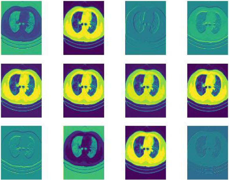
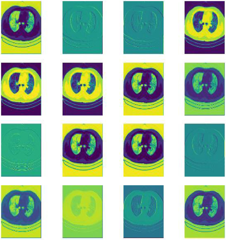
Abstract

The 2019 novel severe acute respiratory syndrome coronavirus 2-SARS-CoV2, commonly known as COVID-19, is a highly infectious disease that has endangered the health of many people around the world. COVID-19, which infects the lungs, is often diagnosed and managed using X-ray or computed tomography (CT) images. For such images, rapid and accurate classification and diagnosis can be performed using deep learning methods that are trained using existing neural network models. However, at present, there is no standardized method or uniform evaluation metric for image classification, which makes it difficult to compare the strengths and weaknesses of different neural network models. This paper used eleven well-known convolutional neural networks, including VGG-16, ResNet-18, ResNet-50, DenseNet-121, DenseNet-169, Inception-v3, Inception-v4, SqueezeNet, MobileNet, ShuffeNet, and EfficientNet-b0, to classify and distinguish COVID-19 and non-COVID-19 lung images. These eleven models were applied to different batch sizes and epoch cases, and their overall performance was compared and discussed. The results of this study can provide decision support in guiding research on processing and analyzing small medical datasets to understand which model choices can yield better outcomes in lung image classification, diagnosis, disease management and patient care.

1. Introduction

COVID-19, a highly infectious lung disease, has caused an extremely serious pandemic that has spread worldwide. Some papers forecast the long-term trajectories of COVID-19 cases using mathematical modeling approaches [1] and stochastic forecasting models [2]. Three important symptoms of COVID-19 are shortness of breath or difficulty breathing, fever, and drying cough [3]. However, in many younger persons, these symptoms might not be present, as a result, other means of detecting infected individuals should be used. Nasal or throat swabs from asymptomatic infected persons are collected, which is uncomfortable and invasive, and then pathological tests such as reverse transcription-polymerase chain reaction (RT-PCR) tests or rapid antigen tests (RAT) are performed on those samples. In addition, diagnosis based on X-ray and computed tomography (CT) chest images is commonly used to assess the severity of the disease and in disease management and patient care [4]. However, identifying COVID-19 from these medical images is time-consuming, challenging, and prone to human errors. As a result, researchers in computer science have developed many automated diagnostic models based on machine learning (ML) or deep learning (DL) to help radiologists improve the accuracy of diagnoses [5] and obtain content performance [6].

In artificial intelligence (AI) methodologies, DL networks are more popular than traditional ML methods. The reason is that, unlike ML techniques, all feature extraction stages, feature selection, and classification are automated in the DL model.

DL generally requires a large amount of training data to enable its network to learn the data characteristics. However, currently, there are two major limitations to using DL on COVID-19 datasets. First, the CT datasets used cannot be shared with the public due to privacy concerns. As a consequence, the DL results cannot be reproduced, and the trained models cannot be used in other hospitals. In addition, the lack of an open-source, annotated COVID-19 CT dataset hinders the research and development of advanced AI methods that can test COVID-19 CT images more accurately. Second, to achieve a performance level that meets clinical standards, using a DL method requires a large number of CT scans to be collected during model training. This requirement is stringent and might not be met by many hospitals, especially since health care professionals are busy caring for COVID-19 patients and are unlikely to have the time to collect and annotate large numbers of COVID-19 CT scans.

In this research, an important finding is that in most papers, it is difficult to quantitatively compare the strengths and weaknesses of the various DL models used on COVID-19 CT scans. This difficulty arises from the lack of standard datasets, networks, indicators, and experimental methods. Another important issue is how to identify a neural network model that can effectively classify small CT datasets. Therefore, eleven well-known convolutional neural networks(CNNs), VGG-16, ResNet-18, ResNet-50, DenseNet-121, DenseNet-169, Inception-v3, Inception-v4, SqueezeNet, MobileNet, ShuffeNet, and EfficientNet-b0, were used to investigate the merits of detecting lung problems in small datasets of COVID-19 patients. This paper notes that these neural network options are not mutually exclusive. In contrast, they can help to guide research or development efforts to understand which model choices can yield better results on small datasets. For the model evaluation and comparison, this research used uniform datasets, data augmentation, hyperparameter training, and consistent optimal weight during the training process. By conducting comparative experiments on the application of the eleven DL models on CT for COVID-19 diagnosis, disease classification, and their variabilities, this research makes the following contributions:

• ●A comprehensive comparative analysis of five performance metrics, namely, accuracy(Acc), recall, precision(Pre), F1, and area under the curve (AUC), were performed on the eleven DL models.
• ●For these eleven models, different batch sizes and epochs and the same five metrics were employed to assess their merits and limitations.
• ●For the traditional neural network models used (ResNet-18, ResNet-50, Dense121, Dense169, Inception-v3, or Inception-v4), this research compared their performance differences under different parameter cases, including different batch sizes and epochs.
• ●The comparative analysis of CNN models conducted in this research on the COVID-19 small datasets can help to guide decision-making and planning recommendations; and help to understand which model choices could yield better transfer learning.

2. Materials and methods

2.1. Deep learning study

2.1.1. VGG

Since winning the ImageNet first runner-up position in 2014, the VGG model has been widely used for image classification. The VGG architecture consists of multiple convolutional layers activated by ReLU (rectified linear unit), and the kernel size of the VGG convolutional layers is chosen to be 3 × 3. VGG-11, VGG-16, and VGG-19 are three variants of the VGG model, which are not very different from each other in terms of the model structure. They consist of successive convolutional and pooling layers, followed by three fully connected layers [7]. They differ only in the number of convolutional layers (11, 16, or 19), which is directly reflected in their names.

In [8], the researchers collected 777 CT images from 88 COVID-19 patients and trained and tested them using VGG. The model had an Acc of 84% with an F1 index of 84% and an AUC of 91%. In Ref. [9], the 150 collected CT images were cut into smaller parts and labeled to form the dataset. The constructed dataset was then trained using the VGG16 network, and two sets of test results were obtained depending on the setting of the dataset, with the optimal set achieving 96.93% accuracy, 99.20% sensitivity, and 94.67% specificity. For this study, VGG-16 was selected.

2.1.2. ResNet

ResNet is a widely used and favored DL network for the identification of COVID-19 CT images. In ResNet and other DL networks, there is a tendency for the accuracy of the model prediction to decrease as the depth increases beyond a certain number, and thus the model depth must be carefully selected. In Ref. [10], this problem was solved by passing features from the lower layers to the higher layers and adding an identity mapping between the higher and lower layers of the network. The main difference between ResNet-18 and ResNet-34 is the multiplier of the block usage, while the main difference between ResNet-34 and ResNet-50 is the internal structure of the block. For this study, ResNet-18 and ResNet-50 neural network models were employed.

In [11], an automated ResNet-based CT image analysis tool for detecting and distinguishing between COVID-19 patients and nonpatients was developed. The results showed an AUC of 99.6%, a sensitivity of 98.2%, and a specificity of 92.2%. In Ref. [12], a total of 618 CT images were collected and used to train the improved model neural network based on ResNet, with a final accuracy of 86.7%. In Ref. [13], the 3D Unet++-ResNet50 combined model was used to classify and identify patients with COVID-19. The final sensitivity and specificity were 97.4% and 92.2%, respectively, and the AUC was 99.1%.

2.1.3. DenseNet

The core of the ResNet model is to train deeper CNNs by establishing shortcuts (skip connections) between the front and back layers, which helps to backpropagate the gradient during training. The DenseNet model is developed based on the same basic idea as ResNet, but it establishes dense connections between all of the previous and subsequent layers, which is reflected in its name [14]. These features allow DenseNet to achieve better performance than ResNet with fewer parameters and less computational cost [15]. DenseNet-121 and DenseNet-169 use the same structure of bottleneck (BN) layers.,i.e., the BN-ReLU-Conv (1 × 1) - BN-ReLU-Conv (3 × 3). The main difference between DenseNet-121 and DenseNet-169 is the multiplier used by the dense block. DenseNet-121 and DenseNet-169 neural network models were used for this study.

In [15], DenseNet was combined with Nu-SVM (support vector machine) to detect COVID-19 pneumonia and achieved a final recall of 90.8%, a precision of 89.7%, and an accuracy of 95.0%. In Ref. [16], DenseNet-121 was used as a control group to compare the results of pneumonia disease classification using Moco self-monitored learning, and the final model achieved an accuracy of 85.5%.

2.1.4. Inception

GoogLeNet, the 2014 ImageNet winner, mainly uses the structure of inception. The main feature of Inception is that it extracts information from different scales of the image through multiple convolutional kernels, finally concatenating them to obtain a better representation of the image [17].

Inception-v2 differs from Inception-v1 in two main ways. The first is the decomposition of the 5 × 5 convolution into two 3 × 3 convolutions. The second is the decomposition of n × n convolutional kernel's size into two convolutions of 1 × n and n × 1. Inception-v3 primarily uses Batch Norm [18]. Inception-v4 introduces a dedicated reduction block, which is used to change the network width and height.

Inception-v4 has a more unified and simplified architecture and more inception modules than Inception-v3 [18].

Inception-v3 was used in Ref. [19] and achieved a final recall of 80.08%, a precision of 80.07%, and an accuracy of 81.63%. In this study, Inception-v3 and Inception-v4 neural network models were used.

2.1.5. SqueezeNet

The core of SqueezeNet is the proposed fire module, which consists of two parts, the squeeze part and the expand part. The squeeze part is a 1 × 1 convolutional kernel and a 1 × 1 convolutional layer. The expand part is 1 × 1 and 3 × 3 convolutional kernels and convolutional layers, respectively. In the expanded layer, the 1 × 1 and 3 × 3 feature maps are concatenated. A comparison on the ImageNet dataset shows that the accuracy of SqueezeNet and AlexNet is roughly equal [20].

In [21], a lightweight CNN model based on SqueezeNet for the recognition of lung CT images, was proposed. The improved model achieved 83% accuracy, 85% sensitivity, 81% specificity, and an F1 value of 0.833 on the test dataset.

2.1.6. MobileNet

The basic unit of MobileNet is the depthwise separable convolution, which can be broken down into two smaller operations: depthwise convolution and pointwise convolution. Depthwise convolution uses different convolution kernels for each input channel, i.e., one convolution kernel for each input channel; thus depthwise convolution is a depth-level operation. The pointwise convolution is just a normal convolution, but it uses 1 × 1 convolution kernels [22].

In [19], the experiments used MobileNet-V1 and obtained a final recall of 88.53%, precision of 88.64%, and accuracy of 89.14%. With MobileNet-V2, the recall was 87.66%, precision was 82.84% and st the accuracy was 85.52%.

2.1.7. ShuffleNet

The design of ShuffleNet accounts for mobile devices with low computing power. The core of ShuffleNet is composed of two operations: pointwise group convolution and channel shuffling, which significantly reduce the computational load of the model while maintaining accuracy. The basic unit of ShuffleNet is demonstrated on the basis of a residual unit [23].

In [24], ShuffleNet was used on X-ray images as raw data, and the final model achieved accuracy, sensitivity, FPR (false-positive rate) and F1 score of 65.26%, 65.26%, 17.36% and 58.79%, respectively.

2.1.8. EfficientNet

To make the neural network model balance the speed and accuracy, EfficientNet combines several dimensions of model scaling: network depth, network width, and image resolution. EfficientNet uses a compound scaling method to find the best combination of these three dimensions, which affect one another [25].

In [26], the EfficientNet model achieved an accuracy of 0.7840 on the test set of 1248 CXR (lung X-ray) images of COVID-19 patients, patients with non-COVID-19-induced pneumonia, and healthy individuals from 2 publicly available datasets.

2.2. Further barriers to comparision

2.2.1. Different datasets

An analysis of the datasets from the relevant literature revealed that except for a few studies that used publicly available datasets, most studies did not provide a detailed description of the chosen data sources. To make the comparison more explicit, this study investigated the datasets that were used in many existing studies. The results are shown in Table 1 .

Table 1.

Different datasets.

Paper	Model	Data source
[8]	VGG-16/DenseNet/ResNet	Images of 88 COVID-19 patients in Wuhan People's Hospital
[24]	ResNet/ShuffleNet DenseNet/MobileNet	These 127 COVID-19 X-ray images were shared by a postdoctoral fellow at the University of Montreal
[26]	VGG-16	A total of 1248 CXR images were obtained from two public datasets, which included 215 images of COVID-19 patients
[9]	VGG-16/GoogleNet/ResNet-50	53 CT images of infected persons provided by the Italian Radiology Association
[27]	ResNet/DenseNet/Inception	CXR images were obtained from two public datasets, which include 236 images of COVID-19 patients
[28]	Inception/ResNet50/MobileNet	Images of 349 confirmed patients and 397 healthy people
[11]	ResNet	The lung CT image data of 157 patients from Chinese hospitals and the United States
[12]	ResNet18	The 618 CT images used were collected from the First Affiliated Hospital of Zheijiang University including 219 images of COVID-19 patients
[13]	Inception/ResNet50/Attention ResNet50	The 1136 (723 COVID-19 positive) training samples were collected from five hospitals including Wuhan Leishenshan Hospital.
[16]	ResNet/DenseNet	The dataset was provided by the Italian Society of Medical and Interventional Radiology
[21]	SqueezeNet	The dataset was provided by the Italian Society of Medical and Interventional Radiology

First, due to patient privacy concerns, hospitals cannot share CT images in their original format, which makes it difficult to reproduce many of the findings. Second, the medical images used in a significant portion of the work in many studies include other forms of imaging, such as X-rays. For many models not trained on a uniform dataset, the trained models can show excellent classification results in some cases, but they might not be robust. Therefore, to conduct a comprehensive comparative analysis of 11 neural networks, this study trained and tested them on a public dataset to ensure the reproducibility of the model training. When researching and analyzing datasets in the relatively small data regime, it also helps to understand which model to choose to obtain desirable results.

2.2.2. Architecture ambiguity

Because some models have many variants, it is difficult to determine the exact network model structure used in some publications, and a typical example is ResNet. For example, in Ref. [12], the classical ResNet-18 network structure for image feature extraction was used. The output of the convolutional layer was flattened to a 256-dimensional feature vector. Then, it was converted to a 16-dimensional feature vector using a fully connected network.

In [19], the ResNet50 model was used to extract features from images. Initially, the ResNet50 model was used to obtain a 1024 dimensional feature map. Then, the SVM was applied to the extracted feature map to classify the sample into two categories. Therefore, in many cases, what is used is a specific neural network model that is a custom variant of the neural network structure. The usual approach is to remove the last few layers of the original neural network and replace them with fully connected layers. In addition, some batch layer, dropout layers, and so on, can also be added.

2.2.3. Different methods of data augmentation

Data augmentation techniques can improve the size and quality of training datasets in such a way that they can be used to build better deep neural network models. In particular, for medical images, creating large medical datasets is very challenging due to the low numbers of patients with specific diseases and the privacy issues of patient data. Therefore, it is necessary to perform data augmentation on medical datasets. Conventional data augmentation methods include geometric transformations, flipping, color space, cropping and rotation. There are also ways to enhance data by developing models, for example, using the popular generative modeling framework to form a generative adversarial network (GAN). In Table 2 , several previously studied image augmentation methods are summarized.

Table 2.

Different methods of data augmentation.

Paper	Data augmentation
[8]	Each set of 3D CT images was equally divided into 15 slices. The slices with incomplete lung were removed. The lung region in each slice was automatically extracted. The images were then filled with a background composed of 10 translational and rotational lungs
[24]	NONE
[26]	The conventional data augmentation method included ± 15° rotation, ± 15% x-axis shift, ± 15% y-axis shift, horizontal flipping, and 85%–115% scaling and shear transformation. The parameters of mixup was set to 0.1
[9]	The original image is divided into 16 * 16 and 32 * 32 blocks to build two data sets
[27]	All the of images were initially preprocessed to have the same size. To make the image size uniform throughout the dataset, each of the images was interpolated using bicubic interpolation.
[28]	The image size was resized to 224 * 224 * 3
[29]	GAN was used for data augmentation. First, the image was resized to 286 * 286, and then it was cropped to 256 * 256 by patchGAN.
[11]	U-net was used to remove the irrelevant areas. Image rotation, horizontal flipping and clipping were used to enhance the data.
[12]	A total of 3957 candidate cubes were generated from the 3D segmentation model. Subsequently, a total of 3957 candidate cubes were generated from the 3D segmentation model.
[13]	Image rotation, horizontal flipping and clipping were used to enhance the data.
[16]	Using random clipping with color distortion to augment data, the size is adjusted
[21]	Rotation (random angle between 0 and 90°), scale (random value between 1.1 and 1.3) and Gaussian noise in the original image were used for data augmentation

2.2.4. Assessment of different metrics

To assess the performance of each DL model, different metrics were applied in different studies to measure their misclassification of COVID-19 in the tested CT images. In Table 3 , the metrics used to evaluate the COVID-19 diagnostic models are summarized. The most commonly used metrics are accuracy and AUC.

Table 3.

Performance criteria.

Paper	Performance Criteria
[8]	AUC\Recall\Precision\F1-score\Accuracy
[24]	Accuracy\Sensitivity\FPR\F1-score
[26]	Accuracy\Sensitivity
[9]	TP\TN\FP\FN\Accuracy \Sensitivity\Specificity\Precision \F1-score\Matthews Correlation Coefficient (MCC)
[27]	\F1-score\Recall\Precision\Specificity
[28]	AUC\Recall\Precision\F1-score\Accuracy
[29]	AUC\Recall\Precision\F1-score\Accuracy
[11]	AUC\Sensitivity\Specificity
[12]	Recall\Precision\F1-score
[13]	AUC\Sensitivity\Specificity
[16]	AUC\Recall\Precision\Accuracy
[21]	AUC\specificity\Precision\F1-score\Accuracy

2.3. Image acquisition

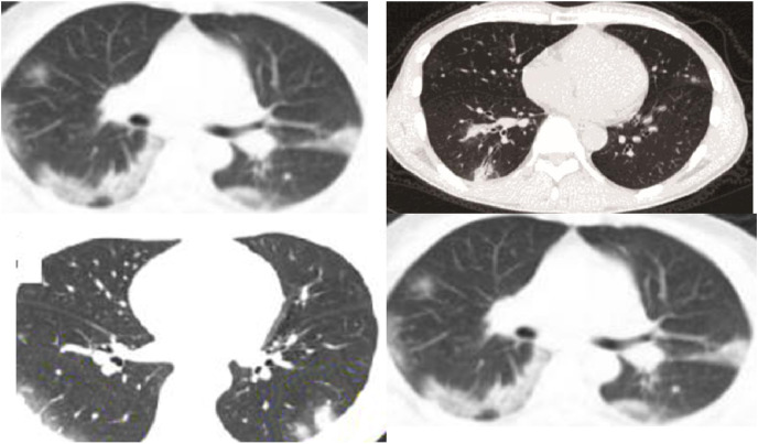
• A:An open-source dataset(UCSD-AI4H) of COVID-19 contains 349 COVID-19 positive CT images and 397 non-COVID-19 CT images from 216 patients. A senior radiologist and experimental studies confirmed the usefulness of the dataset (https://github.com/UCSD-AI4H/COVID-CT). The dataset is available for download at (https://github.com/UCSD-AI4H/COVID-CT). The 349 COVID-19 positive CT images used in this research have different sizes, with the mean, maximum and minimum heights being 491, 1853 and 153, respectively. In addition, the mean, maximum and minimum widths were 383, 1485 and 124, respectively. Fig. 1 shows some examples of COVID-19 CT images.
• B:Another open-source dataset (Italiancase) with 338 COVID-19 CT images is available, and it can be downloaded at (https://www.sirm.org/category/senza-categoria/covid-19/).

Fig. 1.

Four examples of UCSD-AI4H CT images that are positive for COVID-19.

2.4. CT image analysis

2.4.1. CT image preprocessing

The UCSD-AI4H dataset includes 349 COVID-19 CTs and 397 non-COVID-19 CTs, and Fig. 1 shows some of its examples. The CT images were resized to 224 × 224. Then, they were divided into training, validation, and test sets by patient ID. Table 4 shows the statistics for these three subdatasets.

Table 4.

UCSD-AI4H dataset split.

Class	Train	Validation	Test	Total
Normal	234	58	105	397
Pneumonia	191	60	98	349

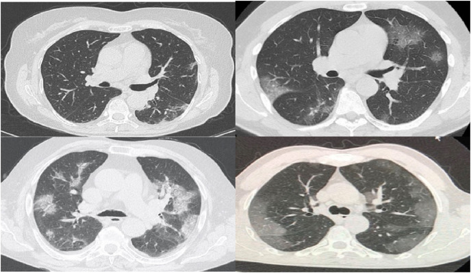
The Italiancase dataset consists of 338 COVID-19 CTs and 397 non-COVID-19 CTs. Fig. 2 shows some of its examples. The size of the CT images was adjusted to 224 × 224. Table 5 shows the statistics for the three subdatasets, including the training, validation, and test sets.

Fig. 2.

Four examples of Italiancase CT images that are positive for COVID-19.

Table 5.

Italiancase dataset split.

Class	Train	Validation	Test	Total
Normal	234	58	105	397
Pneumonia	190	56	92	338

In Fig. 3 the histograms of the pixel intensities of all of the CT scan images in the two datasets after normalization are depicted.

Fig. 3.

Histogram plots of the normalized pixel intensities for the images.

2.4.2. Data augmentation

An important problem with training neural networks on small datasets is that the trained models do not perform well on the validation and test datasets. In order to solve the overfitting problem of these models, a variety of methods have been produced, the simplest of which is to add regularization terms to the weighting paradigm [30]. Another popular technique is dropout, which is achieved by probabilistically removing neurons from a given layer during training or by discarding certain connections [31]. Data augmentation is another way to reduce the overfitting of models. Currently, a widespread and well-accepted practice of image data augmentation is geometric and color augmentation [32], such as reflecting the image, cropping and translating the image, changing the color palette of the image, color processing, and geometrical transformations (rotation, resizing, and so on.). Image augmentation algorithms [33] include geometric transformations, color space augmentations, kernel filters, random erasing, adversarial training, and meta-learning [33]. Among them, the basic methods of image processing data augmentation are geometric transformations, flipping, color space, cropping, rotation, and color space transformations.

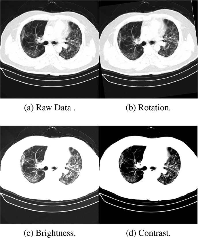
In [32], the dataset from tiny-imagenet-200 was used in one experiment to select pictures of dogs and cats in a binary classification task. The result shows that without any data augmentation, the accuracy was 85.5% on the validation set. After using traditional data augmentation methods, the accuracy was improved to 89%, which indicates that traditional data augmentation has some limited effect on improving the accuracy. The image augmentation methods used in this study are all basic methods. The input images were standardized to have zero mean and unit standard deviation. Then, they were cropped to 224 × 224 × 3. For the UCSD-AI4H dataset and Italiancase dataset, the data augmentation methods and values used for each image are shown in Table 6 .

Table 6.

Data augmentation.

Operation Name	Range
Contrast	[0.9,1.1]
Brightness	[0.9,1.1]
Rotate	[-10,10]

Fig. 4 shows several examples after data augmentation, including changing the brightness and contrasting the image or rotating it.

Fig. 4.

Example transformations after data augmentation.

2.5. Parameter numbers and hyperparameters

2.5.1. Parameter numbers

As shown in Table 7 , this paper listed the statistics of the number of parameters of the eleven selected models.

Table 7.

Comparison of parameter numbers.

Model	Number of model parameters
Vgg-16	138,357,544
ResNet-18	11,177,538
ResNet-50	23,512,130
Dense121	6,955,906
Dense169	12,487,810
inception-v3	21,789,666
inception-v4	41,287,330
SqueezeNet	736,450
MobileNet	2,226,434
ShuffleNet-v2	343,842
efficientNet-b0	44,578

2.5.2. Network hyperparameters

In addition to image preprocessing, hyperparameters are an essential part of neural network training. The hyperparameters of the final model used in this work are listed in Table 8 .

Table 8.

Network hyperparameters.

Hyperparameter	Options
Cost function	Binary cross entropy
Learning rate (Lr)	0.001
Optimizer	Adam
Epochs	800,1500
Batch Size	10,25
Lr Decay	10 times after a plateau

2.6. Neural network training

• (1)
  Training process

  • a)
    A batch of data is obtained from the training dataset to train the model and to input the trained neural network model.
  • b)
    The model outputs bicategorical results, calculates the loss function using cross-entropy, and updates the network weights using the Adam optimizer.
  • c)
    After each epoch, the model parameters are saved, and the model is used to classify the validation set to obtain the F1-score, accuracy, and AUC.
  • d)
    Determine if the best result is the current result according to the numerical value. If so, save an additional copy of the current model parameters;
  • e)
    Steps a-d are repeated until the maximum training epoch is reached.
• (2)Optimal weights of the model saved during the training phase

The optimal weight files generated during the training of the model are selectively recorded. The Accuracy, AUC, and F1-score values obtained by the model on the validation set are written into a dictionary after each training generation. The current values of accuracy, AUC, and F1-score are compared with their corresponding optimal historical values. If a value is greater than its corresponding optimal historical value, the optimal historical value is updated. At the same time, the optimal weight file for this generation of training is saved. Therefore, after the final training, three optimal weight files are obtained, including the Accuracy weight file, the AUC weight file, and the F1 weight file.

2.7. Evaluation metrics

The confusion matrix illustrated in Table 9 is determined. The confusion matrix has four expected outcomes, including true positive (TP), true negative (TN), false positive (FP), and false negative (FN). TP is the number of predicted positives (e.g., predicted as having a disease) and actual positives (e.g., actually having the disease). TN is the number of predicted negatives (e.g., predicted not having a disease) and actual negatives (e.g., not having the disease). FP is the number of predicted positives (e.g., predicted having a disease) but actual negatives (e.g., not having the disease). FN is the number of predicted negatives (e.g., predicted not having a disease) but actual positives (e.g., having the disease).

Table 9.

Confusion matrix.

	Predicted Positive	Predicted Negative
Actual Positive	True Positive (TP)	False Negative (FN)
Actual Negative	False Positive (FP)	True Negative (TN)

For the judgment of the training results of this research, the following five metrics were selected, which are the supporting data for calculating the overall performance metrics.

• 1.Precision is the ratio of the number of positives predicted correctly(TP) to the total number of positives predicted(TP + FP). Precision is specific to the predicted outcome, and this metric reflects how well the model learns about the positive sample characteristics. The higher the precision is, the more accurate the prediction of the positive sample.

$$\text{Precision }=\frac{\mathrm{T}\mathrm{P}}{\mathrm{T}\mathrm{P}+\mathrm{F}\mathrm{P}}$$

• 2.Recall is the percentage of the number of positives predicted correctly (TP) to the total number of actual positives (TP + FN). The higher the recall rate is, the more accuracy the target sample is predicted, and the less likely it is that a bad sample will be missed.

$$\text{Recall}=\frac{\mathrm{T}\mathrm{P}}{\mathrm{T}\mathrm{P}+\mathrm{F}\mathrm{N}}$$

• 3.The F1-score measures the accuracy of a test and is the harmonic mean of the precision and recall. In general, there is a contradiction between the precision and the recall, as a result, F1-score is introduced as a composite index to balance the effects of precision and recall and to evaluate classifier more a correctly.

$$\mathrm{F}1-\mathrm{s}core=2\left(\frac{\text{ Precision }\times \text{ Recall}}{\text{ Precision }+\text{ Recall}}\right)$$

• 4.Accuracy is the ratio of the number of correctly classified samples to the total number of samples. In our study, since it is a binary-classification problem and the number of positive and negative samples is not balanced, the pursuit of high accuracy alone might not reflect the classification effect objectively.

$$Accuracy=\frac{\mathrm{T}\mathrm{P}+\mathrm{T}\mathrm{N}}{\mathrm{T}\mathrm{P}+\mathrm{F}\mathrm{P}+\mathrm{F}\mathrm{N}+\mathrm{T}\mathrm{N}}$$

• 5.AUC (Area Under Curve) is defined as the area under the ROC (receiver operating characteristic) curve, and it is not greater than 1. The ROC curve and AUC are often used to evaluate a binary classifier's effectiveness.

3. Results

To make a comprehensive comparison of the performance of 11 neural networks on the COVID-19 dataset, this study analyzed and compared these models with different batch sizes and epochs. The batch size affects the direction of the gradient descent during backpropagation. The larger the batch size is, the more representative it is of the dataset's overall characteristics, and the faster it converges. However, in terms of computing power, it also requires more memory capacity and more time. In summary, this study chose 10 and 25 for the batch size, respectively. Epochs, another important hyperparameter, do not have a clear criterion in the training process of neural networks. When the periods are too small, the model cannot be adequately trained, which leads to poor performance. In addition, when the epochs are too large, an overfitting issue can arise. In this case, the model tends to perform very well on the training set. However, in fact, it does not learn the actual features of the image, and the classification performance on the test set is significantly reduced.

3.1. Overall performance evaluation on the UCSD-AI4H dataset

Fig. 5, Fig. 6, Fig. 7, Fig. 8, Fig. 9, Fig. 10, Fig. 11, Fig. 12 shows the results of five metrics (Precision, Recall, F1-score, Accuracy and AUC) for the comparison of the 11 models using different optimal weights on 2 COVID-19 datasets, UCSD-AI4H and Italiancase. In the case of the same parameter set, the results of using three different optimal weights were compared horizontally. In most cases, using three different optimal weights with the same epoch and batch size has little effect on the five metrics' results. However, in certain situations, it can have a large effect. For example, on the UCSD-AI4H dataset with epoch = 800 and batch size = 25, when EfficientNet-b0 uses the weights of the optimal accuracy, the accuracy is 76%, and when is uses the weights of the optimal AUC, the accuracy is 67%. Longitudinally, for the same dataset, the final results of the five metrics on the test set using different epochs and batch size parameters are different. However, from the overall comparison of the 11 models, the models’ performance on the five metrics is the same.

Fig. 5.

The overall performance comparison of 11 neural networks on the UCSD-AI4H dataset, with epoch = 800,batch-size = 10.

Fig. 6.

The overall performance comparison of 11 neural networks on the UCSD-AI4H dataset, with epoch = 800,batch-size = 25.

Fig. 7.

The overall performance comparison of 11 neural networks on the UCSD-AI4H dataset, with epoch = 1500,batch-size = 10.

Fig. 8.

The overall performance comparison of 11 neural networks on the UCSD-AI4H dataset, with epoch = 1500,batch-size = 25.

Fig. 9.

The overall performance comparison of 11 neural networks on the Italiancase dataset, with epoch = 800, batch-size = 10.

Fig. 10.

The overall performance comparison of 11 neural networks on the Italiancase dataset, with epoch = 800, batch-size = 25.

Fig. 11.

The overall performance comparison of 11 neural networks on the Italiancase dataset, with epoch = 1500, batch-size = 10.

Fig. 12.

The overall performance comparison of 11 neural networks on the Italiancase dataset, with epoch = 1500, batch-size = 25.

3.2. Overall performance evaluation on italiancase dataset

Overall, on the UCSD-AI4H dataset, EfficientNet-b0 achieved the best performance. On the Italiancase dataset, EfficientNet-b0, ResNet-18, ResNet-50, DenseNet-121, DenseNet-169, Inception-V3 and Inception-V4 all achieved good performance.

4. Discussion

4.1. Calculate comprehensive indicators

To determine the performance of the 11 models in a comprehensive and accurate way, this research considered how to use these five metrics (precision, recall, F1-score, accuracy, and AUC) in combination. However, several of these five metrics are related to each other. Among them, the Fl-score is a combined indicator of the accuracy and recall. It was also observed that some models performed well according to the recall but poorly according to the accuracy and precision, which indicates that the models actually performed poorly. Therefore, to evaluate the merits of the models in a more comprehensive way, the standard deviations (std) and the dispersion of the 4 indicators (precision, recall, accuracy, and AUC) were introduced. This research first added up (sum) the four indicators for each model, then obtained their std, and added a constant k = 0.02 to the obtained std (to make std + 0.02). The last two numbers were then divided to obtain the comprehensive evaluation indicator (sum/(std+0.02)). The process is displayed as follows.

• Step 1Delete F1-score.
• Step 2Calculate Sum = Accuracy + Precision + Recall + AUC
• Step 3Calculate std = std(Accuracy + Precision + Recall + AUC)
• Step 4Calculate sum/(std + 0.02). This value is the comprehensive indicator required.

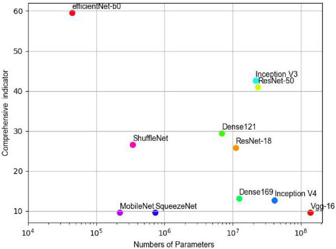
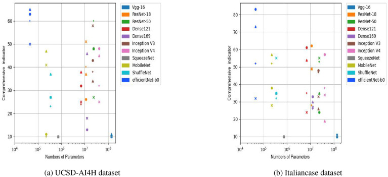
For the image classification task, in addition to the classification effect being the most important index, the number of model parameters was also used as an index to evaluate the merits of the model. Therefore, this research combined these two factors to list the efficiency-effects plot (Fig. 13 ), where the horizontal coordinate is the number of parameters of the model and the vertical coordinate is the overall performance index of the model. The closer the point representing the model is to the upper left corner of the efficiency-effects graph, the better and more efficient the model is. The opposite is true for models near the lower right corner. It can be seen that the EfficientNet-b0 model had the best performance in terms of overall metrics and had smaller model training parameters. The ResNet-18, ResNet-50, DenseNet-121, DenseNet-169, Inception-V3 and Inception-V4 models had moderate performance in terms of overall metrics. The VGG and SqueezeNet models had the worst performance.

Fig. 13.

Comparison of the comprehensive indicators of 11 neural networks for the UCSD-AI4H dataset, with epoch = 800,batch-size = 10.

4.2. Comparison of comprehensive indicators of 11 neural network models

This research employed the composite evaluation indicators mentioned above to compare the performance of each model. By performing the 11 models on the UCSD-AI4H dataset and Italiancase dataset, respectively, with a combination of 2 parameters (batch-size and epochs) and evaluating their performance based on the four sets of parameters, this research obtained the result for the UCSD-AI4H dataset (Fig. 14 (a)), and the result for the Italiancase dataset (Fig. 14 (b)).

Fig. 14.

Comparison of the comprehensive indicators of 11 neural networks. Dot means epoch = 800, batch-size = 10. Plus sign means epoch = 800, batch-size = 25. Triangle means epoch = 1500, batch-size = 25. Cross means epoch = 1500, batch-size = 10.

From the above observation, the 11 neural networks were grouped into four categories.

• ●The first category is Vgg-16 as a baseline methodology.
• ●The second category is ResNet-18, ResNet-50, DenseNet-169, DenseNet-121, Inception-v3, and Inception-v4.
• ●The third category is the SqueezeNet, MobileNet, and ShuffleNet-v2 lightweight models.
• ●The fourth class is EfficientNet-b0, which can scale the model on three parameters: depth, breadth, and input resolution.

Based on the above categorization of the models and the results shown in Fig. 14, the following five conclusions were made.

• 1.The VGG-16 had the worst overall performance.
• 2.SqueezeNet had the worst performance among the SqueezeNet, MobileNet, and ShuffleNet-v2 lightweight models.
• 3.MobileNet and ShuffleNet both outperformed SqueezeNet. MobileNet even achieved performances comparable to those of the ResNet, DenseNet, and Inception series but had the advantage of one order of magnitude fewer parameters.
• 4.The ResNet, DenseNet, and Inception series had no significant advantages over MobileNet and ShuffleNet under certain circumstances. However, the former three classes of models required larger numbers of parameters.
• 5.The EfficientNet-b0 model performs well in a variety of metrics.

On the two small datasets, the EfficientNet model performed better than the ResNet, DenseNet, and the Inception series of networks in terms of the accuracy, synthesis, and efficiency. Similar results were obtained when compared to those shown in Ref. [34]. MobileNet achieved a performance comparable to ResNet, DenseNet, and the Inception series on the two small datasets.

4.3. Different batch-size, epoch parameters on ResNet, DenseNet, and inception series models

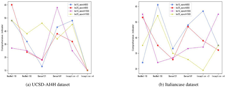
In this section, this research determined the general effect of the batch size and epoch parameters on the six ResNet, DenseNet, and Inception series models. The combined metrics of these six models in four different parameter combinations (batch size: 10 and 25; epoch: 800 and 1500) are shown in Fig. 15 .

Fig. 15.

Comparison of comprehensive indicators under different batch sizes and epoch parameters on ResNet, DenseNet, and Inception series models.

According to Fig. 15, the following two conclusions were obtained. First, a model with more layers might not have better performance, e.g., in the UCSD-AI4H dataset case, the overall performance of ResNet18 was better than ResNet50 in all four cases. In the Italiancase dataset, the overall performance of ResNet18 was better than ResNet50 in 2 out of 4 cases.

Second, a larger number of model parameters does not necessarily produce better overall model performance. For example, for the Inception series, the number of model parameters of Inception-v4 was greater than that of Inception-v3. In the case of the UCSD-AI4H dataset, in all four cases, Inception-v3 performed better than Inception-v4 in terms of the overall performance. In the case of the Italiancase dataset, in two of the four cases, Inception-v3 performed better than Inception-v4.

In [10], the top-1 errors of ResNet18 and ResNet34 on the ImageNet dataset were compared. The fact that ResNet34 had a lower error rate than ResNet18 indicated that ResNet34 performed better than ResNet18. In Ref. [15], on the ImageNet dataset, DenseNet 169 was less error-prone than DenseNet 121. In Ref. [35] on the ImageNet dataset, Inception-v3 was less error-prone than Inception-v4.

Through the two small datasets used in this study, for the ResNet, DenseNet, and Inception models, it can be found that a larger number of layers of the model does not necessarily give better performance.

To further investigate these two findings, this research evaluated the image quality of the ImageNet dataset, the UCSD-AI4H dataset, and the Italiancase dataset. Image quality assessment can generally be divided into two types: the subjective quality score given by managers and the objective quality score given by the image quality model. Subjective quality assessment methods would be more accurate. Nevertheless, because they are expensive, time-consuming, and unsuitable for large-scale data, algorithms should be investigated to predict the image quality. Current objective quality assessment methods are roughly divided into three categories, including full reference image quality assessment (FRIQA), reduced reference image quality assessment (RRIQA), and no reference image quality assessment (NRIQA) [36]. Among them, NRIQA is a so-called blind image quality assessment (BIQA).

Compared to other image assessment methods, the NRIQA method does not require the original distortion-free reference image, which fits most application scenarios; therefore, the NRIQA method was employed in this study. Compared with the BIQA method, the FRIQA method has developed a complete theoretical system and assessment model. The most commonly used indicators in FRIQA are the mean square error (MSE) based on pixel statistics, peak signal-to-noise ratio (PSRN), and structural similarity (SSIM) based on structural information [37].

The generic BIQA algorithm learns to map from image features to the corresponding quality fractions or to split the image into different distortion categories before mapping. Since the first use of natural scene statistics (NSS) [38] for image quality assessment in 2005, many experiments have shown that there is a close relationship between NSS features and image quality. In 2012, Mittal et al. proposed another model for extracting NSS features in the spatial space: the Blind/Referenceless Image Spatial Quality Evaluator (BRISQUE) [39].

The data quality of the Imagenet dataset, the UCSD- AI4H dataset, and the Italiancase dataset was evaluated using four metrics: MSE, PSNR, SSIM, and BRISQUE, and the results are shown in Table 10 .

Table 10.

Imagenet, UCSD-AI4H and Italiancase Image quality assessment.

	Imagenet	UCSD-AI4H	Italiancase
MSE	8264	13804	10645
PSNR	6.81	6.75	6.45
SSIM	0.145	0.172	0.142
BRISQUE	15.31	17.35	29.89

From Table 10, it can be seen that the PSNR and SSIM values are low. The image was selected as the reference image (ref) inside the LIVE dataset. The smaller the MSE result is, the smaller the gap between the detected image and the reference image. The BRISQUE result is a number between 0 and 100, and the smaller the number is, the better the quality. According to the MSE and BRISQUE metrics, the image data quality of the Imagenet dataset is better than that of the UCSD-AI4H and Italiancase datasets. Therefore, for the UCSD-AI4H dataset and the Italiancase dataset, more layers of the model and the more model parameters do not mean that the overall performance of the model is better. The likely reason is the poor quality of the dataset, which ultimately leads to the overfitting of the model.

This result can be used to extend classification studies on small image datasets to other areas. There are still some limitations to this study. First, the image quality of the two datasets was not high, and it was difficult for the neural network model to learn the features of the local pneumonia foci. Second, there were no clinical features associated with neocoronary pneumonia to examine the correlations between the symptoms and the pneumonia lesion characteristics.

4.4. Comparison of results before and after data augmentation

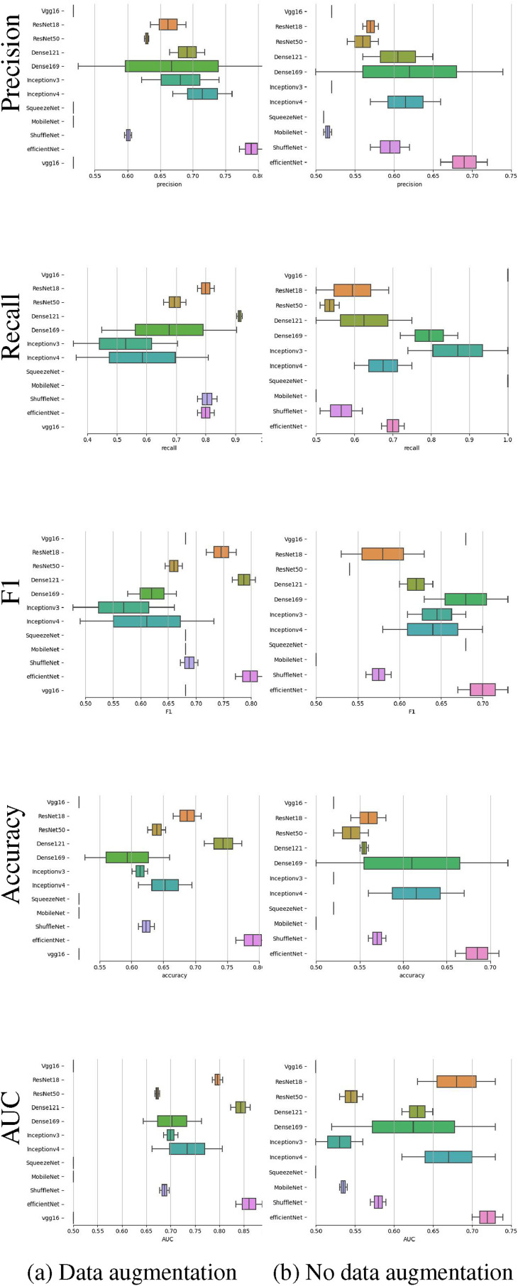
The contrast experiment for data augmentation and no data augmentation is performed on the UCSD-AI4H dataset. The boxplots of precision, recall, f1, accuracy and AUC are plotted in Fig. 16 . The experimental results show that after data augmentation, the accuracy of the test set and each metric without data augmentation are improved accordingly.

Fig. 16.

Boxplots of precision, recall,F1, accuracy and AUC for the UCSD-AI4H dataset in 2 experiments with data augmentation and without data augmentation.

4.5. Visualization interpretability

In recent years, deep neural networks (DNNs) have made great achievements in natural language processing, computer vision, and other applications. Their performance is not only better than a number of existing machine learning methods but also outstanding when addressing actual tasks.

With the intention of opening the black-boxes of DNNs, a number of scholars have paid attention to the interpretability of the model. Although many studies have explored this topic, there is currently no unified definition of interpretability. Moreover, the definitions and motivations of interpretability that they proposed are usually diverse or even significantly inconsistent with one another.

It can be noted that several papers have distinguished between explainability and interpretability. In this research, the minute variance between these two concepts was not considered. As defined above, this research considered the explanation to be the essence of interpretability; and used understandability, explainability, and interpretability interchangeably. Specifically, this research attempted to study the interpretability of DNNs, with the purpose of providing an explanation of their internal operations as well as input-output mappings.

The main functions of using feature visualization to explore the working mechanism of a deep convolution neural network are as follows:

• 1.It is helpful to understand and analyze the working principle and decision-making process of the neural network to better select or design the network. For example, for classification networks, CAM places higher requirements on the network in addition to the classification accuracy. Specifically, it not only requires high prediction accuracy, but also requires the network to extract the required features.
• 2.It makes use of visual information to guide the network to achieve better learning results.

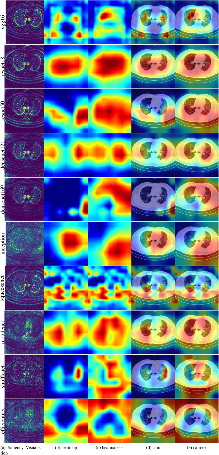
Among the interpretation forms of neural networks, methods based on saliency are the most commonly used. These methods assign importance weights to each pixel of the input image to indicate the significance of each pixel to the predicted category of the image. The saliency map [40] can be considered to be a feature map, which demonstrates the influence of the pixels in the image on the result of image classification.

The full name of CAM is Class Activation Mapping [41], also known as the Category Heat Map; In general, it is represented by a grayscale image from 0 to 255 with the same size as the original picture, and the pixel value of each position on it ranges from 0 to 1. It can be understood as the contribution distribution to the prediction output. The higher the value is, the higher the response and the greater the contribution of the corresponding area of the original picture to the network. The visualization of CAM can be presented in the form of a superposition of the heat map and the original image. The darker the red is, the greater the value. It can be considered that when the network predicts the “COVID-19” category, the red highlighted area is its primary bias for judgment.

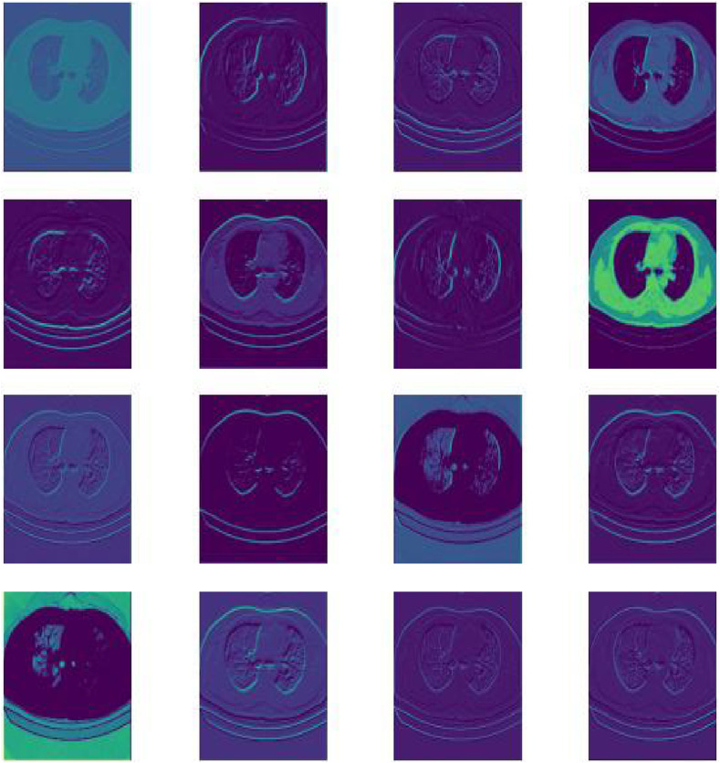
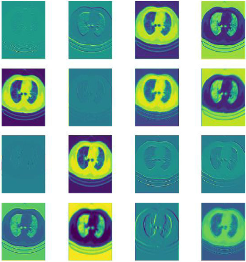
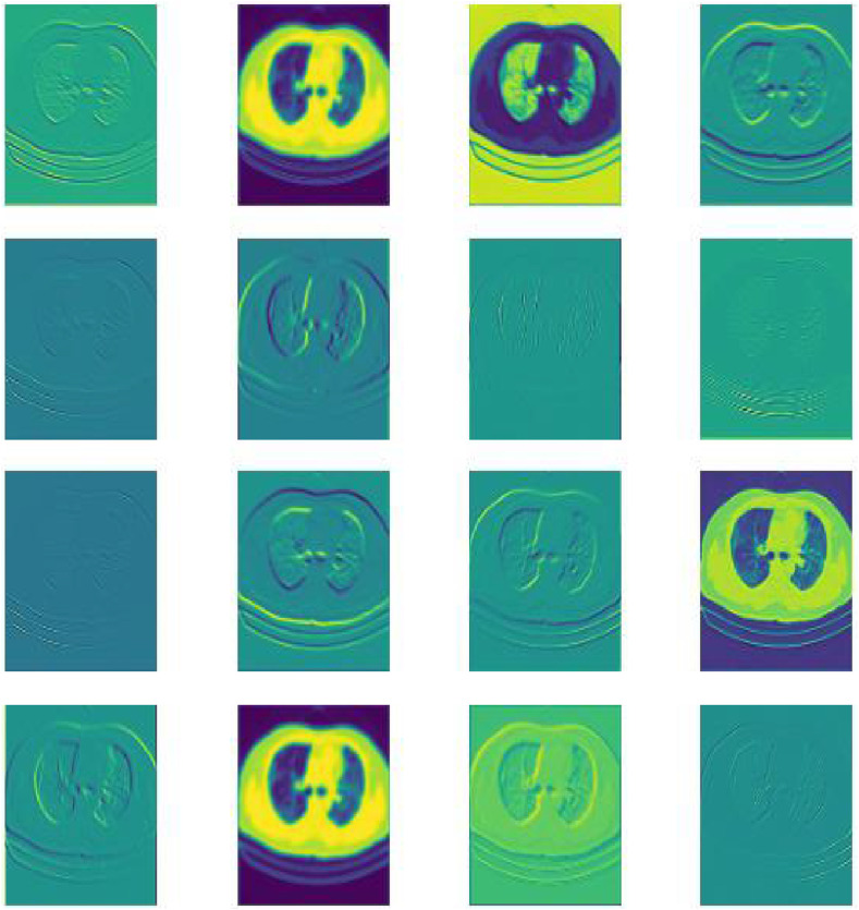
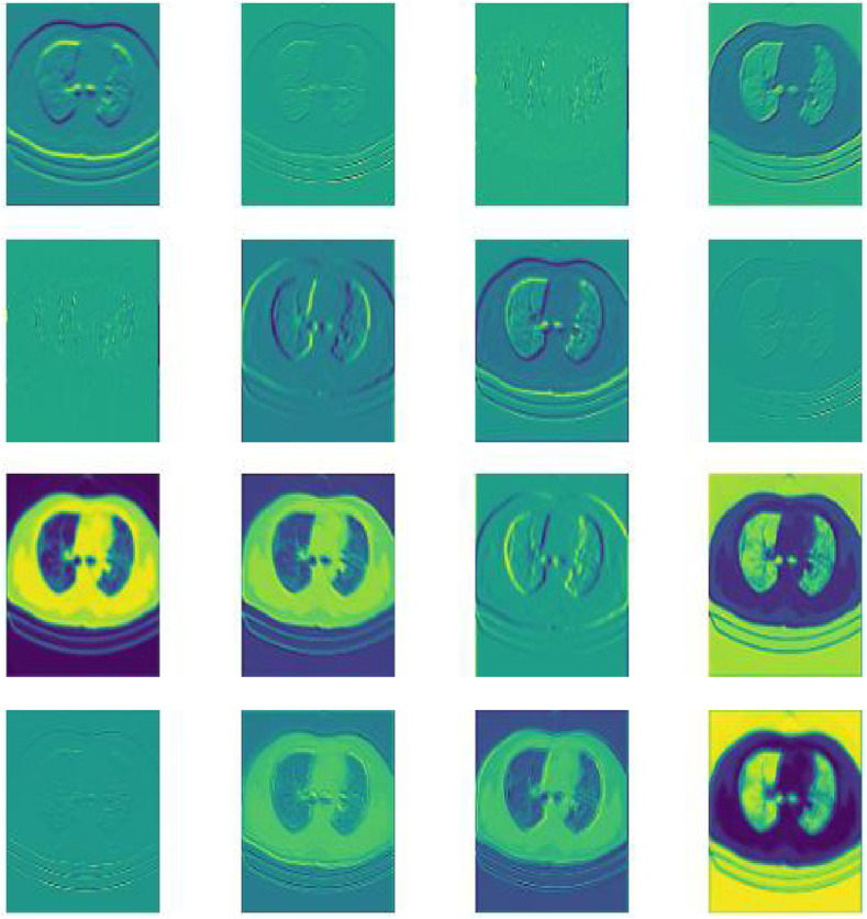
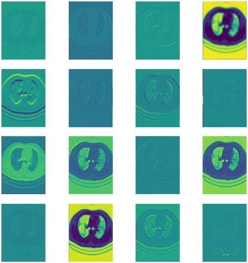
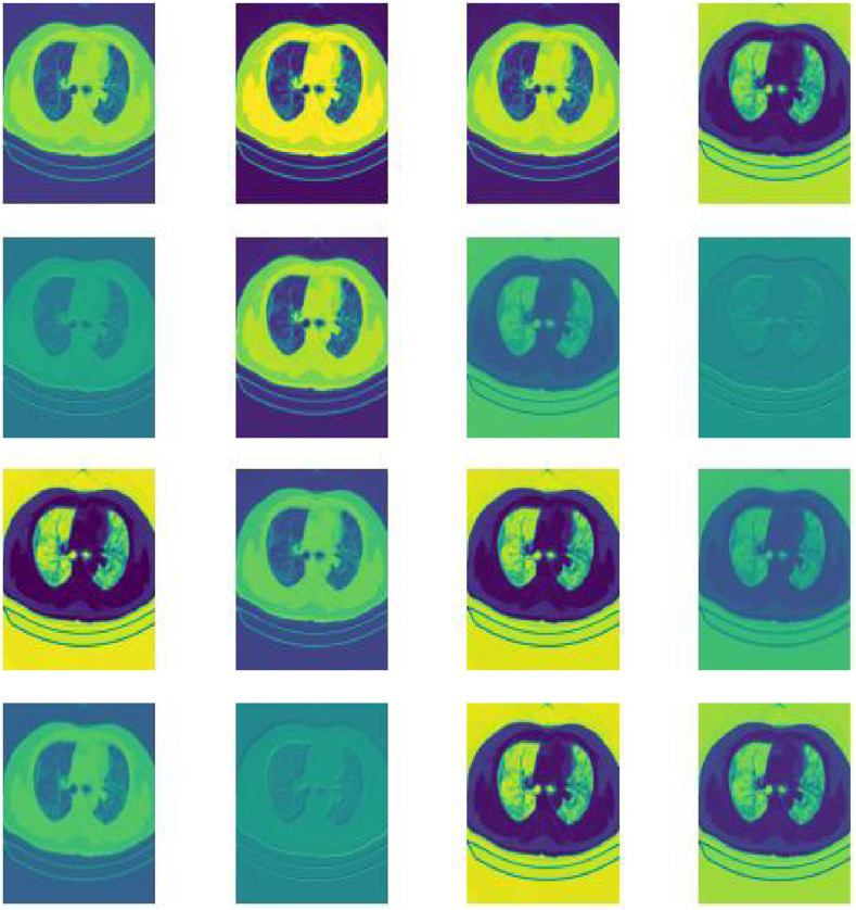
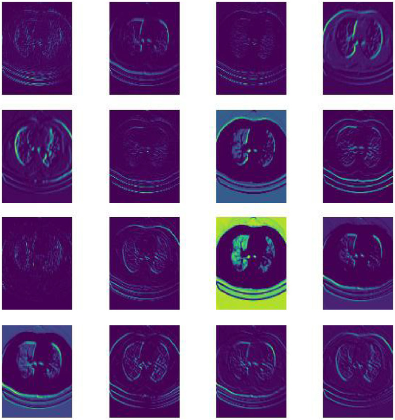
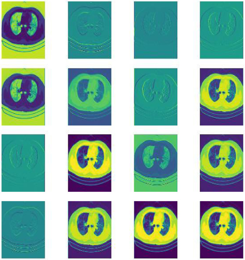
The intuitive visualization is to draw the weight of the target layer. The weights visualization [42] of the first layer are presented in Appendix A. In general, the coverage areas of the heatmap and CAM are similar, as in Fig. 17 . Therefore, the renderings presented by the CAMs of each neural network were discussed separately.

• ●Saliency maps of VGG, Resnet, and Denset pay more attention to local features; MobileNet, ShuffeNet, and SqueezeNet do not perform well in extracting key features; EffcientNet performs well not only in paying attention to global features, but also in distinguishing key features.
• ●The Grad-CAMs of VGG-16 and SqueezeNet do not cover the entire object. In contrast, those of Resnet, Denset, Inception, and EffcientNet have more comprehensive coverage. This finding further illustrates that the performance of the Resnet, Denset, Inception, and EffcientNet models is better than that of the VGG-16 and SqueezeNet models.
• ●Compared with Grad-CAM, the objects covered by Grad-CAM++ [43] are more comprehensive. The objects covered by Grad-CAM are only partial, while Grad-CAM++ covers almost all objects. In particular, the Grad-CAM++ of the Resnet, Denset, and EffcientNet models can basically cover all objects.

Fig. 17.

Visualization interpretability for learned features from several methods.

5. Conclusions

This research studied the effect of 11 neural networks on learning on the COVID19-CT dataset, and evaluated the performance of the random initialization network. In addition, the differences in the final classification performance of the neural network models on the COVID19-CT dataset were compared. The results of this research can guide researchers and help them determine the most suitable model, and understand the conditions under which the models will produce better results. This paper contributes to a systematic comparison and evaluation of the performance of 11 traditional neural network models in a relatively small data regime. For the relatively small data regime, a neural network model that has deeper layers does not necessarily provide better overall performance. In general, choosing neural networks with residual connectivity (e.g. ResNet) and automatic search capability (e.g. EfficientNet) gives better results. It should be noted that neural network models impact the model performance when using different hyperparameters. However, in general, neural networks with residual connections (e.g., ResNet) and automatic search capabilities (e.g., EfficientNet) have better migration performance.

Appendix A. Weights visualization

To deeply understand the behavior of 11 neural networks using weight visualization, visual explanations of the predictions of convolutional neural networks are provided. The weight visualization of the first layer is presented in Fig. A.18 to Fig. A.27. As output, the weights of the current layer were obtained to be grayscale images, and 16 of them were plotted. According to these images, certain pixels at the edges of the image are brighter than others.

Fig. A.18.

weights-01layer-vgg16.

Fig. A.19.

weights-01layer-resnet18.

Fig. A.20.

weights-01layer-resnet50.

Fig. A.21.

weights-01layer-densenet121.

Fig. A.22.

weights-01layer-densenet169.

Fig. A.23.

weights-01layer-inception-v3.

Fig. A.24.

weights-01layer-squeezenet.

Fig. A.25.

weights-01layer-mobilenet.

Fig. A.26.

weights-01layer-shufflenet.

Fig. A.27.

weights-01layer-efficientnet.

References

- 1.Ritu Y., Gupta Numerical analysis approach for models of Covid-19 and other epidemics. Int. J. Model. Simulat. Sci. Comput. 2021 doi: 10.1142/S1793962320410032. [DOI] [Google Scholar]
- 2.Ghosh I., Chakraborty T. An integrated deterministic–stochastic approach for forecasting the long-term trajectories of COVID-19. Int. J. Model. Simulat. Sci. Comput. 2021:2141001doi. doi: 10.1142/S1793962321410014. https://www.worldscientific.com/doi/abs/10.1142/S1793962321410014 [DOI] [Google Scholar]
- 3.Sohrabi C., Alsafi Z., O'Neill N., Khan M., Kerwan A., Al-Jabir A., Iosifidis C., Agha R. World Health Organization declares global emergency: a review of the 2019 novel coronavirus (COVID-19) Int. J. Surg. 2020;76:71–76. doi: 10.1016/j.ijsu.2020.02.034. https://linkinghub.elsevier.com/retrieve/pii/S1743919120301977 [DOI] [PMC free article] [PubMed] [Google Scholar]
- 4.Kadry S., Rajinikanth V., Rho S., Raja N.S.M., Rao V.S., Thanaraj K.P. 2020. Development of a Machine-learning System to Classify Lung CT Scan Images into Normal/COVID-19 Class.http://arxiv.org/abs/2004.13122 arXiv:2004.13122. [Google Scholar]
- 5.Ulhaq A., Khan A., Gomes D., Paul M. 2020. Computer Vision For COVID-19 Control: A Survey; pp. 1–24.http://arxiv.org/abs/2004.09420 arXiv:2004.09420. [DOI] [PMC free article] [PubMed] [Google Scholar]
- 6.Wu X., Hui H., Niu M., Li L., Wang L., He B., Yang X., Li L., Li H., Tian J., Zha Y. Deep learning-based multi-view fusion model for screening 2019 novel coronavirus pneumonia: a multicentre study. Eur. J. Radiol. 2020;128(April):1–9. doi: 10.1016/j.ejrad.2020.109041. [DOI] [PMC free article] [PubMed] [Google Scholar]
- 7.Simonyan K., Zisserman A. ICLR 2015 - Conference Track Proceedings. 2015. Very deep convolutional networks for large-scale image recognition, 3rd International Conference on Learning Representations; pp. 1–14. [Google Scholar]
- 8.Song Y., Zheng S., Li L., Zhang X., Zhang X., Huang Z., Chen J., Zhao H., Jie Y., Wang R., Chong Y., Shen J., Zha Y., Yang Y. 2020. Deep Learning Enables Accurate Diagnosis of Novel Coronavirus (COVID-19) with CT Images. [DOI] [PMC free article] [PubMed] [Google Scholar]
- 9.Ozkaya U., Ozturk S., Barstugan M. 2020. Coronavirus (COVID-19) Classification Using Deep Features Fusion and Ranking Technique; pp. 1–13. [Google Scholar]
- 10.He K., Zhang X., Ren S., Sun J. 2016 IEEE Conference on Computer Vision and Pattern Recognition (CVPR) IEEE; 2016. Deep residual learning for image recognition; pp. 770–778.http://ieeexplore.ieee.org/document/7780459/ [DOI] [Google Scholar]
- 11.Gozes O. 2020. Rapid AI Development Cycle for the Coronavirus (COVID-19) Pandemic: Initial Results for Automated Detection & Patient Monitoring Using Deep Learning CT Image Analysis. [Google Scholar]
- 12.Xu X., Jiang X., Ma C. Applied Intelligence; 2020. Deep Learning System to Screen Coronavirus Disease 2019 Pneumonia; pp. 1–29. [DOI] [PMC free article] [PubMed] [Google Scholar]
- 13.Jin S., Wang B., Xu H., Luo C., Wei L., Zhao W., Hou X., Ma W., Xu Z., Zheng Z., Sun W., Lan L., Zhang W., Mu X., Shi C., Wang Z., Lee J., Jin Z., Lin M., Jin H., Zhang L., Guo J., Zhao B., Ren Z., Wang S., You Z., Dong J., Wang X., Wang J., Xu W. 2020. AI-assisted CT Imaging Analysis for COVID-19 Screening: Building and Deploying a Medical AI System in Four Weeks; pp. 1–22. [DOI] [PMC free article] [PubMed] [Google Scholar]
- 14.Lee C.Y., Xie S., Gallagher P.W., Zhang Z., Tu Z. Deeply-supervised nets. J. Mach. Learn. Res. 2015;38:562–570. [Google Scholar]
- 15.Huang G., Liu Z., Van Der Maaten L., Weinberger K.Q. 2017 IEEE Conference on Computer Vision and Pattern Recognition (CVPR) 2017. Densely connected convolutional networks; pp. 2261–2269. [Google Scholar]
- 16.Chen X., Yao L., Zhou T., Dong J., Zhang Y. 2020. Momentum Contrastive Learning for Few-Shot COVID-19 Diagnosis from Chest CT Images. [DOI] [PMC free article] [PubMed] [Google Scholar]
- 17.Szegedy C., Liu Wei, Jia Yangqing, Sermanet P., Reed S., Anguelov D., Erhan D., Vanhoucke V., Rabinovich A. 2015 IEEE Conference on Computer Vision and Pattern Recognition (CVPR) IEEE; 2015. Going deeper with convolutions; pp. 1–9.http://ieeexplore.ieee.org/document/7298594/ [DOI] [Google Scholar]
- 18.Szegedy C., Vanhoucke V., Ioffe S., Shlens J., Wojna Z. Proceedings of the IEEE Computer Society Conference on Computer Vision and Pattern Recognition 2016-Decem. 2016. Rethinking the inception architecture for computer vision; pp. 2818–2826. arXiv:1512.00567. [DOI] [Google Scholar]
- 19.Saeedi A., Saeedi M., Maghsoudi A. 2020. A Novel and Reliable Deep Learning Web-Based Tool to Detect COVID-19 Infection from Chest CT-Scan. [Google Scholar]
- 20.Iandola F.N., Han S., Moskewicz M.W., Ashraf K., Dally W.J., Keutzer K. 2016. SqueezeNet: AlexNet-level Accuracy with 50x Fewer Parameters and <0.5MB Model Size; pp. 1–13. [Google Scholar]
- 21.Polsinelli M., Cinque L., Placidi G. 2020. A Light CNN for Detecting COVID-19 from CT Scans of the Chest; pp. 1–13. [DOI] [PMC free article] [PubMed] [Google Scholar]
- 22.Howard A.G., Zhu M., Chen B., Kalenichenko D., Wang W., Weyand T., Andreetto M., Adam H., MobileNets . 2017. Efficient Convolutional Neural Networks for Mobile Vision Applications. [Google Scholar]
- 23.Ma N., Zhang X., Zheng H.T., Sun J. 2018. Shufflenet V2: Practical Guidelines for Efficient CNN Architecture Design, Lecture Notes in Computer Science (including subseries Lecture Notes in Artificial Intelligence and Lecture Notes in Bioinformatics) 11218 LNCS; pp. 122–138. [DOI] [Google Scholar]
- 24.Sethy P.K., Behera S.K., Ratha P.K., Biswas P. Detection of coronavirus disease (COVID-19) based on deep features and support vector machine. Int. J. Math. Eng. Manage. Sci. 2020;5(4):643–651. doi: 10.33889/IJMEMS.2020.5.4.052. [DOI] [Google Scholar]
- 25.Tan M., Le Q.V., EfficientNet . 36th International Conference on Machine Learning. ICML; 2019. Rethinking model scaling for convolutional neural networks; pp. 10691–10700. 2019 2019-June. [Google Scholar]
- 26.Nishio M. Vol. 1. 2020. pp. 6–8. (Automatic Classification Between COVID-19 Pneumonia, Non-COVID-19 Pneumonia, and the Healthy on Chest X-ray Image: combination of Data Augmentation Methods in a Small Dataset). [DOI] [PMC free article] [PubMed] [Google Scholar]
- 27.Chatterjee S., Saad F., Sarasaen C., Ghosh S., Khatun R., Radeva P., Rose G., Stober S., Speck O., Nürnberger A. 2020. Exploration of Interpretability Techniques for Deep COVID-19 Classification Using Chest X-Ray Images. [DOI] [PMC free article] [PubMed] [Google Scholar]
- 28.Saeedi A., Saeedi M., Maghsoudi A. 2020. A Novel and Reliable Deep Learning Web-Based Tool to Detect COVID-19 Infection from Chest CT-Scan.http://arxiv.org/abs/2006.14419 arXiv:2006.14419. [Google Scholar]
- 29.Mobiny A., Cicalese P.A., Zare S., Yuan P., Abavisani M., Wu C.C., Ahuja J., de Groot P.M., Van Nguyen H. 2020. Radiologist-Level COVID-19 Detection Using CT Scans with Detail-Oriented Capsule Networks. [Google Scholar]
- 30.Wang B., Klabjan D. 2016. Regularization for Unsupervised Deep Neural Nets.http://arxiv.org/abs/1608.04426 arXiv:1608.04426. [Google Scholar]
- 31.Kubo Y., Tucker G., Wiesler S. 2016. Compacting Neural Network Classifiers via Dropout Training.http://arxiv.org/abs/1611.06148 arXiv:1611.06148. [Google Scholar]
- 32.Perez L., Wang J. 2017. The Effectiveness of Data Augmentation in Image Classification using Deep Learning.http://arxiv.org/abs/1712.04621 arXiv:1712.04621. [Google Scholar]
- 33.Shorten C., Khoshgoftaar T.M. A survey on image data augmentation for deep learning. J. Big Data. 2019;6(1):60. doi: 10.1186/s40537-019-0197-0. https://journalofbigdata.springeropen.com/articles/10.1186/s40537-019-0197-0 [DOI] [PMC free article] [PubMed] [Google Scholar]
- 34.Howard A., Sandler M., Chen B., Wang W., Chen L.C., Tan M., Chu G., Vasudevan V., Zhu Y., Pang R., Le Q., Adam H. Proceedings of the IEEE International Conference on Computer Vision 2019-Octob. 2019. Searching for mobileNetV3; pp. 1314–1324. arXiv:1905.02244. [DOI] [Google Scholar]
- 35.Szegedy C., Ioffe S., Vanhoucke V., Alemi A.A. 31st AAAI Conference on Artificial Intelligence. AAAI; 2017. Inception-v4, inception-ResNet and the impact of residual connections on learning; pp. 4278–4284. 2017. arXiv:1602.07261. [Google Scholar]
- 36.Wang Z., Bovik A.C. Modern image quality assessment, synthesis lectures on image. Video, and Multimedia Processing. 2006;2(1):1. doi: 10.2200/S00010ED1V01Y200508IVM003. http://www.morganclaypool.com/doi/abs/10.2200/S00010ED1V01Y200508IVM003 156. [DOI] [Google Scholar]
- 37.Sara U., Akter M., Uddin M.S. Image quality assessment through FSIM, SSIM, MSE and PSNR—a comparative study. J. Comput. Commun. 2019:8–18. doi: 10.4236/jcc.2019.73002. 07 (03) [DOI] [Google Scholar]
- 38.Sheikh H., Bovik A., Cormack L. No-reference quality assessment using natural scene statistics: JPEG2000. IEEE Trans. Image Process. 2005;14(11):1918–1927. doi: 10.1109/TIP.2005.854492. http://ieeexplore.ieee.org/document/1518954/ [DOI] [PubMed] [Google Scholar]
- 39.Mittal A., Moorthy A.K., Bovik A.C. No-reference image quality assessment in the spatial domain. IEEE Trans. Image Process. 2012;21(12):4695–4708. doi: 10.1109/TIP.2012.2214050. http://ieeexplore.ieee.org/document/6272356/ [DOI] [PubMed] [Google Scholar]
- 40.Simonyan K., Vedaldi A., Zisserman A. ICLR 2014 - Workshop Track Proceedings. 2014. Deep inside convolutional networks: visualising image classification models and saliency maps, 2nd International Conference on Learning Representations; pp. 1–8. arXiv:1312.6034. [Google Scholar]
- 41.Selvaraju R.R., Cogswell M., Das A., Vedantam R., Parikh D., Batra D. Grad-CAM: visual explanations from deep networks via gradient-based localization. Int. J. Comput. Vis. 2020;128(2):336–359. doi: 10.1007/s11263-019-01228-7. arXiv:1610.02391. [DOI] [Google Scholar]
- 42.Zeiler M.D., Fergus R. 2014. Visualizing and Understanding Convolutional Networks, Lecture Notes in Computer Science (including subseries Lecture Notes in Artificial Intelligence and Lecture Notes in Bioinformatics) 8689 LNCS (PART 1) pp. 818–833. arXiv:1311.2901. [DOI] [Google Scholar]
- 43.Chattopadhay A., Sarkar A., Howlader P., Balasubramanian V.N. Proceedings - 2018 IEEE Winter Conference on Applications of Computer Vision, WACV 2018 2018-January. 2018. Grad-CAM++: Generalized gradient-based visual explanations for deep convolutional networks; pp. 839–847. arXiv:arXiv:1710.11063v3. [DOI] [Google Scholar]