ADAPTIVE IMPORTANCE SAMPLING VIA AUTO-REGRESSIVE GENERATIVE MODELS AND GAUSSIAN PROCESSES

Abstract

The quality of importance distribution is vital to adaptive importance sampling, especially in high dimensional sampling spaces where the target distributions are sparse and hard to approximate. This requires that the proposal distributions are expressive and easily adaptable. Because of the need for weight calculation, point evaluation of the proposal distributions is also needed. The Gaussian process has been proven to be a highly expressive non-parametric model for conditional density estimation whose training process is also straightforward. In this paper, we introduce a class of adaptive importance sampling methods where the proposal distribution is constructed in a way that Gaussian processes are combined autoregressively. By numerical experiments of sampling from a high dimensional target distribution, we demonstrate that the method is accurate and efficient compared to existing methods.

1. INTRODUCTION

Adaptive importance sampling (AIS) is a class of powerful estimation methods that iteratively optimize the proposal distribution along with drawing weighted samples. There are many different variations of AIS; however the performance of all these methods is very sensitive to the quality of the chosen proposal distribution [18]. Traditionally, fixed parametric distributions, such as Gaussian mixtures, are used as proposal distributions [2, 16]. However, in high dimensional samples spaces, the target distributions are usually hard to be captured by these fixed-form distributions.

With the development of machine learning, several kinds of compound data generating methods have proven to be highly expressive, such as neural generative models [6, 14] and Gaussian process latent variable machines [20]. These methods succeed in capturing details of high dimensional data distributions. However, to use data generating methods as proposal distributions for AIS, point evaluations of the generative models are required to calculate the weights of the drawn samples. However, many data generating models cannot evaluate the probability analytically. For example, in [22], a variational autoencoder (VAE) model is used as a proposal distribution, where the probability is evaluated by Monte Carlo approximations.

There are two kinds of compound distributions that can evaluate probability of samples analytically. One is latent variable machines that use bidirectional transformations [5, 11, 15, 21]. The other kind of distributions, which are called autoregressive distributions, are the ones that can be factorized by the chain rule of conditional distributions. In [13], it was shown that these two types of models are equivalent under certain conditions. In this paper, we work within the autoregressive framework.

Kernel density estimation is a commonly used non-parametric density estimation method, and it is usually invoked in low dimension sample spaces. In terms of estimation of conditional distributions, there are several methods such as [9, 10]. Gaussian processes allow for a powerful non-parametric conditional density estimation, where the models of the data are conditional Gaussian distributions.

In this paper, we introduce a class of AIS methods that use autoregressive distributions whose components are non-parametric distributions, including kernel density estimation and Gaussian processes, as proposal distributions. We provide two examples of this class of methods, and they are based on AIS and adaptive multiple importance sampling (AMIS). By numerical experiments, we show that when the dimension of the target distribution is high, the proposed methods outperform the state-of-the-art AMIS methods and Gaussian mixture distributions.

The problem is defined in Section 2. In Section 3, we briefly review AIS, autoregressive distributions, and Gaussian processes. We propose our method in Section 4 and present results of numerical experiments in Section 5. In Section 6, we discuss the results and provide concluding remarks.

2. PROBLEM DEFINITION

Our goal is to draw samples from a given non-normalized target distribution π(x). We assume that we can only evaluate π(x) point-wisely. We also assume that the integral of π(·) is not tractable and that as a result, the partition function is not available. This is a common situation in Bayesian estimation when we want to draw samples from a posterior distribution: the partition function of a high-dimensional posterior distribution is usually not available.

When x is high dimensional, the target distribution is sparse, and the sampling process is very challenging. We address the problem of sampling from target distributions of this type.

3. BACKGROUND

3.1. Adaptive importance sampling and its variations

We operate in settings when we do not have much information about the target distribution π(x), and thus, handcrafting a proposal distribution q(x) for importance sampling (IS) is challenging [8]. AIS is a class of iterative importance sampling that optimizes the proposal distribution over iterations of IS [12]. We will use the subscript t to denote the iteration index. We start from some initialization of the proposal distribution q₁(x), and in each importance iteration t, we use the accumulated weighted samples ($X_{1:t}^{(m)}$,$w_{1:t}^{(m)}$), to optimize an updated proposal distribution q_t+1(x). This step is called “adaptation.” There are many ways of adaptation, depending on the form of the proposal distribution. Proceeding with iterations, we improve the proposal distribution, and thereby the quality of the drawn samples and the various statistics obtained from them.

Variations of AIS methods [2], such as AMIS [4] are usually different because of the adopted form of the proposal distribution, the process of adaptation, and how the results from previous iterations are used. Many of these methods use Gaussian or Gaussian mixture distributions as proposal distributions [3, 4]. The accuracy of these methods degrades fast with the increase of the dimension of the sample space. Therefore, an expressive proposal distribution that can approximate the target distribution better in higher dimensions is needed.

3.2. Autoregressive distributions

Autoregressive distributions are joint distributions that can be factorized based on the conditional distribution expansion rule,

$$q_t\left(x_t\right)=q_{1,t}\left(x_{1,t}\right)\prod _{d=2}^D{q}_{d,t}\left(x_{d,t}\mid x_{1:d-1,t}\right),$$ (1)

where D is the number of dimensions of the sample space. Samples of this distribution can be drawn by ancestral sampling [1]. Evaluation of the log-probability of a sample can be achieved by separately computing the factors corresponding to each dimension, and the sum of the evaluations is the log-probability of that sample. When optimizing the autoregressive distribution, each factor of the proposal distribution can be optimized separately in parallel.

3.3. Gaussian processes

The Gaussian process regression [23] is a non-parametric Bayesian model for estimation of functions from noisy data. They rely on conditional Gaussian distributions, where their covariances are regulated by “kernels” that measure similarities among data.

Suppose that training input and output data are given by (x^(1:N), y^(1:N)), where N is the number of training data. The predictive distribution of y* conditioned on x* is modeled by

$$q\left(y^{*}\mid x^{*},\theta ,{\sigma }^2\right)=\mathcal{N}\left(y^{*}\mid {\mu }_t\left(x^{*},\theta \right),{\Sigma }_t\left(x^{*},\theta \right)+{\sigma }^2\right),$$ (2)

where

$$\begin{gathered} {\mu }_t\left(x^{*},\theta \right)={\Sigma }_{*,x}{\left({\Sigma }_{x,x}+{\sigma }^2{I}_N\right)}^{-1}{y}^{(1:N)}, \\ {\Sigma }_t\left(x^{*},\theta \right)={\Sigma }_{*,*}-{\Sigma }_{*,x}{\left({\Sigma }_{x,x}+{\sigma }^2{I}_N\right)}^{-1}{\Sigma }_{*,x}^{\top }\text{,} \end{gathered}$$

and

$$\begin{gathered} {\Sigma }_{x,x}=\left[\begin{array}{ccc}{k}_{\theta }\left(x^{(1)},x^{(1)}\right)& \cdots & k_{\theta }\left(x^{(1)},x^{(N)}\right)\\ ⋮& \ddots & ⋮\\ k_{\theta }\left(x^{(N)},x^{(1)}\right)& \cdots & k_{\theta }\left(x^{(N)},x^{(N)}\right)\end{array}\right], \\ {\Sigma }_{*,\text{x}}=\left[\begin{array}{lll}{k}_{\theta }\left(x^{*},x^{(1)}\right)\hfill & \cdots \hfill & k_{\theta }\left(x^{*},x^{(N)}\right)\hfill \end{array}\right], \\ {\Sigma }_{*,*}=k_{\theta }\left(x^{*},x^{*}\right), \end{gathered}$$

where θ and σ² are hyperparameters of the GP model, and k_θ(·, ·) is the kernel function of the GP. In the proposed method, we use the radial basis function (RBF) kernel.

However, it is hard for the GP to work with large datasets because the inverse of the covariance matrix requires O(N³) complexity. There are many methods that aim to reduce the computational complexity of Gaussian process regression [17]. In our work, we utilize a python package GPy [7] that uses the deterministic training conditional (DTC) approximation [19] to reduce the computational complexity to O(n³) where n is the number of inducing input, and n is much smaller than the data size N.

4. THE PROPOSED METHOD

4.1. AIS with non-parametric proposals

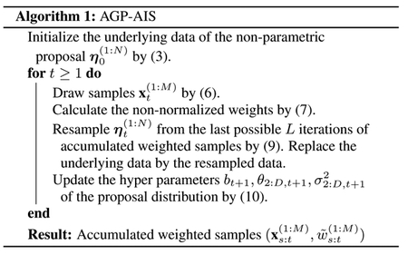
In the proposed AIS method, the proposal distribution has the autoregressive form (1). Because the proposal distribution is non-parametric, in the initialization step, we need to provide some initialization of the underlying data ${\eta }_{1:D,0}^{(1:N)}$. Here we can use random data drawn from a non-informative distribution, such as a standard Gaussian distribution,

$${\eta }_{1:D,0}^{(1:N)}\stackrel{iid}{~}\mathcal{N}\left(0,I_D\right),$$ (3)

where N is the number of drawn samples, and I_D denotes the D-by-D identical matrix.

The distribution of the first dimension q_1,t(x_1,t) can be modeled by kernel density approximation, which is non-parametric. Kernel density estimation is usually not challenging in low dimensional spaces. As we are using it for just one dimension, it will be suitable for modeling the distribution of the first dimension,

$$q_{1,t}\left(x_{1,t}\right)=\frac{1}{N}\sum _{n=1}^N\mathcal{N}\left(x_{1,t}\mid {\eta }_{1,t-1}^{(n)},b_t^2\right),$$ (4)

where b_t is the bandwidth of the smoothing kernel at iteration t.

The conditional distributions are modeled by Gaussian processes according to (2), with (${\eta }_{1:d-1,t}^{(1:N)}$, ${\eta }_{d,t}^{(1:N)}$) as underlying input and output training data, or

$$\begin{gathered} q_{d,t}\left(x_{d,t}\mid x_{1:d-1,t},{\theta }_{d,t},{\sigma }_{d,t}^2\right)= \\ \mathcal{N}\left(x_{d,t}\mid {\mu }_t\left(x_{1:d-1,t},{\theta }_{d,t}\right),{\Sigma }_t\left(x_{1:d-1,t},{\theta }_{d,t}\right)+{\sigma }_{d,t}^2\right). \end{gathered}$$ (5)

When sampling from a distribution, we first draw samples from the kernel density approximation and then we generate samples from the conditional distributions sequentially, i.e.,

$$\begin{gathered} k_t^{(1:M)}\stackrel{iid}{~}\mathcal{D}\mathcal{U}(1:N), \\ {x}_{1,t}^{(m)}~\mathcal{N}\left({\eta }_{1,t-1}^{\left(k_t^{(m)}\right)},b_t^2\right), \\ {x}_{d,t}^{(m)}~\mathcal{N}\left(x_{d,t}\mid {\mu }_t\left(x_{1:d-1,t}^{(m)},{\theta }_{d,t}\right),{\Sigma }_t\left(x_{1:d-1,t}^{(m)},{\theta }_{d,t}\right)+{\sigma }_{d,t}^2\right), \end{gathered}$$ (6)

where $\mathcal{D}\mathcal{U}(1:N)$ means discrete uniform distribution that samples integers from 1 to N.

The non-normalized sample weights are calculated by

$${\tilde{w}}_t^{(m)}=\text{exp}\left(\text{log}\left(\pi \left(x_t^{(m)}\right)\right)-\text{log}\left(q_t\left(x_t^{(m)}\right)\right)\right),m=1:M,$$ (7)

where the log-pdf evaluation of the proposal distribution is

$$\begin{gathered} \text{log}\left(q_t\left(x_t^{(m)}\right)\right)=\text{log}\left(\frac{1}{N}\left[\sum _{n=1}^N\mathcal{N}\left(x_{1,t}^{(m)}|{\eta }_{1,t-1}^{(n)},b_t^2\right)\right]\right) \\ +\sum _{d=2}^D\mathcal{L}\mathcal{N}\left(x_{d,t}^{(m)}\mid {\mu }_t\left(x_{1:d-1,t}^{(m)},{\theta }_{d,t}\right),{\Sigma }_t\left(x_{1:d-1,t}^{(m)},{\theta }_{d,t}\right)+{\sigma }_{d,t}^2\right), \end{gathered}$$ (8)

and $\mathcal{L}\mathcal{N}$ denotes the log-pdf of a Gaussian distribution.

The proposal distribution is non-parametric, and therefore adaptations can be achieved by replacing the underlying data set of the proposal distribution with resampled data from the accumulated weighted samples. Note that the number of resampled samples N does not have to be the same as the number of samples drawn from the proposal distribution M. The resampling process can be performed as follows:

$$\begin{gathered} i_t^{(1:N)}\stackrel{iid}{~}\mathcal{C}\left(s:t,\frac{{\sum }_{l=1}^M{\tilde{w}}_{s:t}^{(l)}}{{\sum }_{r=s}^t{\sum }_{l=1}^M{\tilde{w}}_r^{(l)}}\right), \\ {j}_t^{(1:N)}\stackrel{iid}{~}\mathcal{C}\left(1:M,\frac{{\sum }_{r=s}^t{\tilde{w}}_r^{(1:M)}}{{\sum }_{r=s}^t{\sum }_{l=1}^M{\tilde{w}}_r^{(l)}}\right), \\ {\eta }_t^{(n)}=x_{i_t^{(n)}}^{\left(j_t^{(n)}\right)},n=1:N, \end{gathered}$$ (9)

where $\mathcal{S}=\text{max}(0,t-L+1)$, and L is the maximum number of iterations that is kept. The earlier iterations are considered as burn-in. The symbols $\mathcal{C}\left(x^{(1:M)},w^{(1:M)}\right)$ denote a categorical distribution from which we draw x according to the weights w.

In addition to replacing the underlying data, we can also update the hyperparameters based on the resampled samples for better performance. The bandwidth of the kernel density estimation, the hyperparameters of the Gaussian process kernel, the white noise of the Gaussian process, and the inducing points can be updated by the type-II maximum likelihood as follows:

$$\begin{gathered} b_{t+1}=\underset{b}{\text{argmax}}\frac{1}{N}\sum _{n=1}^N\text{log}\left(q_{1,t}\left({\eta }_{1,t}^{(n)},b\right)\right), \\ {\theta }_{d,t+1},{\sigma }_{d,t+1}^2=\underset{{\theta }_d,{\sigma }_d^2}{\text{argmax}} \\ \frac{1}{N}\sum _{n=1}^N\text{log}\left(q_{d,t}\left(x_{d,t}^{(n)}\mid x_{1:d-1,t}^{(n)},{\theta }_{d,t},{\sigma }_{d,t}^2\right)\right). \end{gathered}$$ (10)

The inducing inputs are optimized by DTC using the GPy [7] package. The proposed AIS method is summarized by Algorithm 1, which we refer to as autoregressive GP AIS (AGP-AIS).

4.2. AMIS with non-parametric proposals

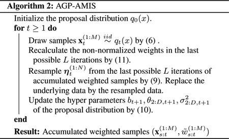
Our non-parametric proposal distribution can be used in different variations of AIS. For example, it can be applied in the AMIS structure if we change the weighting process of AIS (7) to the following:

$${\tilde{w}}_j^{(m)}=\frac{(t-s+1)\pi \left(x_t^{(m)}\right)}{{\sum }_{i=s}^t{q}_i\left(x_t^{(m)}\right)}j=s:t,m=1:M,$$ (11)

where q_i is the exponent of (8). Note that in each iteration t, we need to re-weight the history samples from iteration s to t. The proposed AMIS method is summarized by Algorithm 2 AGP-AMIS.

5. NUMERICAL EXPERIMENTS

The target distribution for all the experiments is a banana-shaped distribution [4], which is defined by

$$\pi (x)=f_{\mathcal{N}\left(0_D,\Sigma \right)}\left(x_1,x_2+b\left(x_1^2-{\sigma }^2\right),x_3,\cdots ,x_D\right),$$ (12)

where Σ = diag(σ², 1, …, 1). In our experiments, we set the parameters to b = 0.03 and σ = 10.

We ran experiments with the proposed AGP-AIS and AGP-AMIS methods. For comparison purposes, we also tested AMIS that uses a Gaussian mixture distribution with 10 components as a proposal distribution.

Even though we only utilize point evaluation of the target distribution, it is actually possible to generate samples from the target distributions directly by first drawing z^(1:M) from a standard Gaussian distribution, and then twist its first two dimensions to acquire x^(1:M), that is to follow these steps:

$$Z^{(1:M)}\stackrel{iid}{~}\mathcal{N}\left(0,I_D\right),$$ (13)

and then, for m = 1 : M

$$\begin{gathered} x_1^{(m)}=\sigma z_1^{(m)}, \\ {x}_2^{(m)}=z_2^{(m)}+b\left({\sigma }^2+{\left(x_1^{(m)}\right)}^2\right), \\ {x}_{3:D}^{(m)}=z_{3:D}^{(m)}. \end{gathered}$$ (14)

In the experiment, the ideal samples are directly drawn from the target distribution for benchmark performance comparisons.

The performance is measured in two ways. First, as suggested in [4], we measure the difference between the following statistics and their theoretical values:

$$P_1=\sum _{d=1}^D\text{mean}\left(x_{d,s:t}^{(1:M)}\right)-\sum _{d=1}^{D}E\left(x_d\right),$$ (15)

$$P_2=\sum _{d=1}^2\text{var}\left(x_{d,s:t}^{(1:M)}\right)-\sum _{d=1}^{2}V\left(x_d\right),$$ (16)

$$P_3=\sum _{d=3}^D\text{var}\left(x_{d,s:t}^{(1:M)}\right)-\sum _{d=3}^{D}V\left(x_d\right).$$ (17)

Second, we focus on the first two dimensions of the samples. Because we know the ideal samples can be acquired transforming the standard Gaussian distribution samples, we can apply the inverse transformation of (14) on samples from the proposed methods and measure the Gaussianity of the inverse transformed samples $T^{-1}\left(x_{s:t}^{(1:M)}\right)$, where T⁻¹(·) is defined by

$$T^{-1}\left(x_{1:2}\right)={\left[\frac{x_1}{\sigma },x_2+b\left({\sigma }^2+x_1^2\right)\right]}^{\top }$$ (18)

The performance is measured by the maximum difference between the sample cumulative distribution function (CDF) and the standard Gaussian CDF, which can be further used in the Kolmogorov–Smirnov Gaussianity test.

We did two sets of experiments. In the first experiment, we used M =1E5 and N =1E3 in all the compared sampling methods. We performed 10 simulations of the methods for target distributions with different dimensions D =5, 10, 15, 20. In this example, we see that the performance decays quickly for GM-AMIS when the number of dimensions increases, while the AGP-based methods remain with very high accuracy.

In the second experiment, we used the same dimension of the target distribution, D =10, and the same number of resampled samples for proposal adaptation N =1E3 for all the tested methods but drew different numbers of samples M =1E3, 1E4, 1E5 from the proposal distribution. In this example, we see that to achieve similar performance, GM-AMIS needs to draw many more samples than the AGP methods.

Because the target distribution becomes sparser in high dimensions, the Gaussian process-based distribution, which is more expressive, can estimate the target distribution better. The method is non-parametric, and it makes full use of the weighted samples. Thus, it needs less samples than the Gaussian mixture-based methods.

6. CONCLUSIONS AND DISCUSSIONS

In this paper, we proposed a class of adaptive importance sampling methods that use auto-regressive generative models and Gaussian processes for obtaining proposal distributions. Our numerical experiments suggest that the methods are efficient in the number of samples, more accurate, and less sensitive in dimensions than existing methods.

Fig. 1:

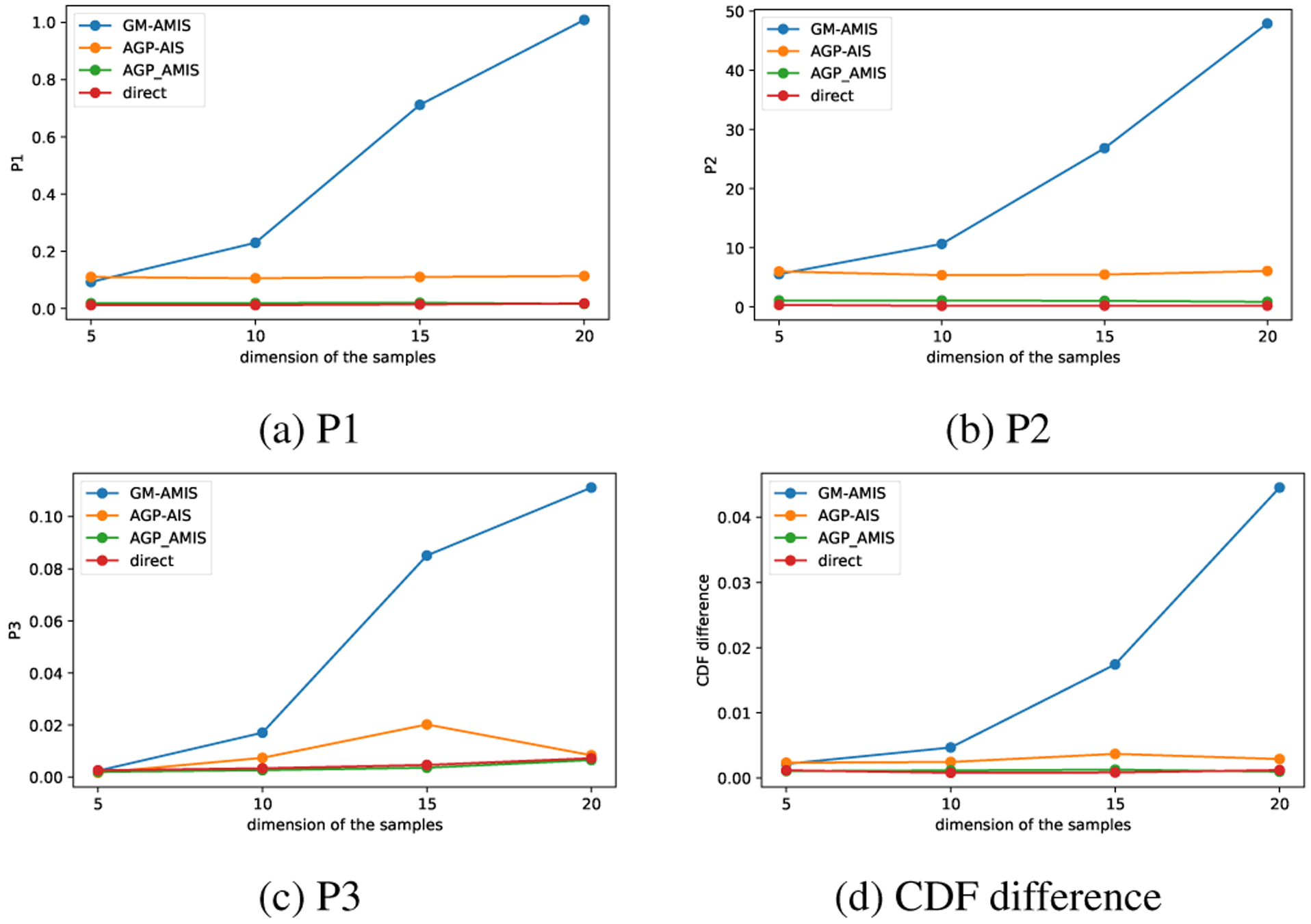
Performance of the methods as a function of the dimension of x. The definitions of P₁, P₂, and P₃ are given by (15)–(17).

Fig. 2:

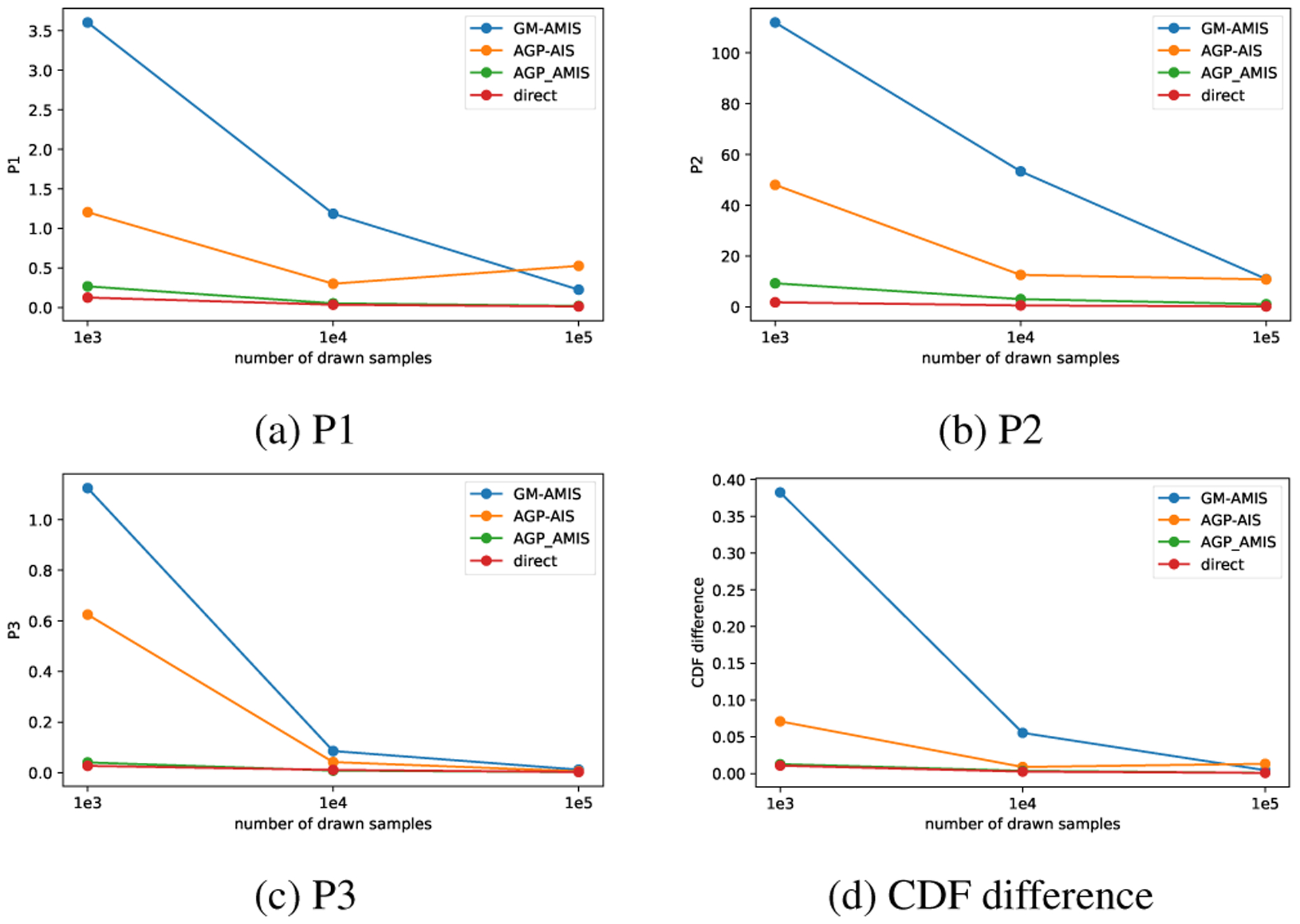
The performance of the methods as functions of the number of drawn samples. The definitions of P₁, P₂, and P₃ are given by (15)–(17).

Fig. 3:

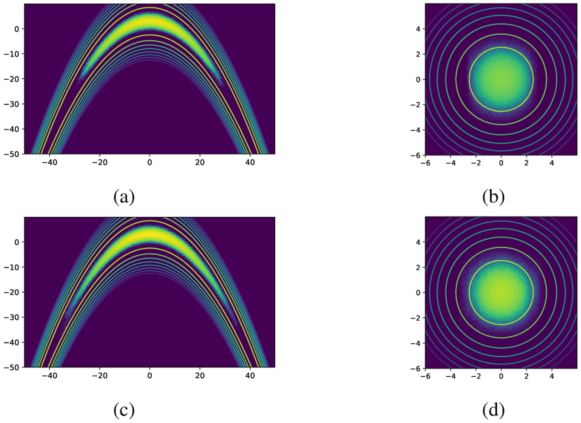
(a) and (c) are log-histograms of the samples acquired from one realization of the proposed methods with 1E5 samples drawn from a 20-dimensional banana-shaped distribution, where (a) is obtained by AGP-AIS and (c) is obtained by AGP-AMIS. The lines are contours of the log target distribution. (b) and (d) are transformed samples from (a) and (c) correspondingly. The lines are contours of the log standard normal distribution.