Assessment of event-triggered policies of nonpharmaceutical interventions based on epidemiological indicators

Abstract

Nonpharmaceutical interventions (NPI) such as banning public events or instituting lockdowns have been widely applied around the world to control the current COVID-19 pandemic. Typically, this type of intervention is imposed when an epidemiological indicator in a given population exceeds a certain threshold. Then, the nonpharmaceutical intervention is lifted when the levels of the indicator used have decreased sufficiently. What is the best indicator to use? In this paper, we propose a mathematical framework to try to answer this question. More specifically, the proposed framework permits to assess and compare different event-triggered controls based on epidemiological indicators. Our methodology consists of considering some outcomes that are consequences of the nonpharmaceutical interventions that a decision maker aims to make as low as possible. The peak demand for intensive care units (ICU) and the total number of days in lockdown are examples of such outcomes. If an epidemiological indicator is used to trigger the interventions, there is naturally a trade-off between the outcomes that can be seen as a curve parameterized by the trigger threshold to be used. The computation of these curves for a group of indicators then allows the selection of the best indicator the curve of which dominates the curves of the other indicators. This methodology is illustrated with indicators in the context of COVID-19 using deterministic compartmental models in discrete-time, although the framework can be adapted for a larger class of models.

Introduction

After the initial outbreak of COVID-19 in Wuhan, China, the novel coronavirus SARS-COV-2 has spread to multiple countries (Li et al. 2020) causing over 183 million cases and almost 4 million deaths by July 4, 2021 (World Health Organization 2021). Since the emergence and global spread of COVID-19 in a context where no approved vaccines, treatments, or prophylactic therapies were still available (Alvi et al. 2020), countries implemented different nonpharmaceutical interventions (NPI) (Flaxman et al. 2020). These prevention, containment, and mitigation policies had been implemented in order to flatten the peak of critical cases and consequently, to prevent as far as possible the health systems from being overwhelmed (Alvi et al. 2020; OECD 2020).

In a scenario where pharmaceutical interventions are not available, public health policy responses to the pandemic aim both to limit the number and duration of social contact. Even in a scenario where pharmaceutical interventions have begun to be implemented, mainly the progressive vaccination of the population, the nonpharmaceutical measures are needed to prevent widespread outbreaks, and therefore have continued to be applied (Moore et al. 2021; Yang et al. 2021). They include measures such as early detection of cases, and tracing and isolating infected individual’s contacts (testing and contact tracing), the use of Personal Protective Equipment (PPE) by health care workers, and social distancing measures, among others (Alvi et al. 2020; OECD 2020). Social distancing interventions include working from home, school closures, cancellation of public gatherings and restrictions on unnecessary movement outside one’s residence such as national or partial lockdowns (Alvi et al. 2020; Davies et al. 2020; Flaxman et al. 2020; OECD 2020). These measures have been shown to be successful in reducing the spread of SARS-COV-2 (Alvi et al. 2020; Flaxman et al. 2020). Lockdowns, in particular, have had a substantial effect on the transmission as measured by the changes in the estimated reproduction number (Flaxman et al. 2020). In fact, a modeling study of the demand for hospital services in the UK found that intermittent periods of more intensive lockdown-type measures are predicted to be effective in preventing health system overload (Davies et al. 2020).

Beyond the health consequences of the pandemic, it also has important economic consequences (Martin et al. 2020; McKibbin and Fernando 2020), throwing many countries into recession and possible economic depression (Brodeur et al. 2020; Kurowski et al. 2021). The economic impact can be direct and indirect (Béland et al. 2020; Brodeur et al. 2020; Fan et al. 2018; Martin et al. 2020; Meltzer et al. 1999), at the individual or aggregate level, affecting firms and different sectors (Martin et al. 2020; Nicola et al. 2020), and with effects in the short, medium and long term (Béland et al. 2020; Brodeur et al. 2020; Gong et al. 2020; Nicola et al. 2020). The negative economic effects may vary based on the severity of the social distancing measures, the length of their implementation, and the degree of compliance (Brodeur et al. 2020), and, as usual, in times of crises the most vulnerable groups are affected the most (Buheji et al. 2020; Marmot and Allen 2020).

Health systems must face direct costs related to the diagnosis and confirmation testing, outpatient and inpatient care, and vaccines and pharmaceutical treatments when these were available (Fan et al. 2018; Meltzer et al. 1999). On the other hand, productivity is affected by both absenteeism (patients and preventive isolation) and deaths caused by the virus (Brodeur et al. 2020; Fan et al. 2018; Meltzer et al. 1999; UNDP 2020).

In this context, authorities are constantly searching for balance between health and economic consequences; with the latter being the result of not only the former but also of the measures or policies implemented to confront the health issues. This is the case for the aforementioned lockdowns that keep the individuals of a certain locality or sector confined and, therefore, reduce the economic activity. Therefore, it is possible to perceive a trade-off between the extension of lockdowns, and its impact on productivity, and the health outcomes observed; for instance, the longer lockdown period, the fewer intensive care units (ICU) required (or number of cases, or deaths). In terms of the objective for the decision makers, it is sought to minimize both the lockdowns duration and the health consequences (Alvarez et al. 2020; Angulo et al. 2021; Grigorieva et al. 2020).

Several countries and cities have used epidemiological indicators to activate, reinstate and release NPI such as lockdowns. In fact, in World Health Organization (2020), has proposed various public health criteria to adjust public health and social measures in the context of COVID-19. The criteria are grouped into three domains: Epidemiology, Health system and Public health surveillance. Many of these criteria can be expressed in terms of the following indicators: effective reproduction number, active new cases, positivity rate, and hospitalization and intensive care unit (ICU) admissions due to COVID-19.

In this context, the government of San Francisco (US) has published on its website (San Francisco government 2020) various health indicators used to monitor the level of COVID-19 in the city and assess the ability of its health care system to respond to the pandemic. These health indicators are grouped into 5 areas: hospital system, cases, testing, contact tracing and personal protective equipment. The first three areas are characterized in terms of the following observations: COVID-19 hospitalizations, acute care beds available, ICU beds available, new cases per day per 100,000 residents, and tests collected per day. The last two areas consider the indicators related to contact tracing and personal protective equipment that are beyond the scope of our study. In other places, such as the city of Austin (US), it was decided to track daily COVID-19 hospital admissions and daily total hospitalizations across the city and trigger the initiation and relaxation of lockdown periods when admissions cross predetermined thresholds (Duque et al. 2020).

In the case of Chile, and in particular its capital, Santiago, which is our main case study, at the beginning of the outbreak the government used indicators mainly based on the active cases (per 100,000 residents and per area) and on the available hospital beds to activate lockdowns (Chilean Ministry of Health 2020). These lockdowns were dynamically applied to the most affected sectors of the cities. Since July 2020, a five-steps plan known as “Paso a Paso" (Step by Step), has been used to release and reinstate various NPI measures including lockdowns (Chilean Government 2020). Following the recommendations of the World Health Organization (2020) and of the COVID-19 advisory council (Aguilera et al. 2020), an independent organism conceived to guide the Chilean Ministry of Public Health in the policies that will be implemented to face the COVID-19 outbreak; this plan now takes into account several dimensions of the pandemic through the monitoring of the following indicators: ICU beds available, effective reproductive number, new active cases, positivity rate, and some additional tracing and surveillance indicators. Thus, lockdowns are now release/reinstate for a given district of a city when the values of these indicators, computed for such districts, are below/above the predetermined thresholds. In this country, the mass vaccination plan started in February 2021 and, as by early July, 10.5 million individuals have been fully vaccinated (Chilean Government 2021). Although four vaccines have been approved for emergency use: Pfizer-BioNTec, CoronaVac (Sinovac), AstraZeneca and CanSino (Chilean Ministry of Health 2021); CoronaVac has been the most used in the country (about 80% of the doses) (Aguilera et al. 2021), and the “Paso a Paso" plan (consisting in several NPIs) continues to be implemented (Chilean Government 2020).

Given the aforementioned situation, our aim is to propose a framework based on control theory that permits to assess and compare NPI policies based on epidemiological indicators.

It is important to note that the application of NPI strategies to mitigate the effects of the COVID-19 pandemic has been already modeled using control theory and other techniques, as fractional models (Aba Oud et al. 2021). For instance, in Djidjou-Demasse et al. (2020) andx Ullah and Khan (2020), optimal control theory is used to explore the best strategy for implementation while waiting for the development of a vaccine. More specifically, in Djidjou-Demasse et al. (2020) the authors seek a solution minimizing deaths and costs due to the implementation of the control strategy while in Ullah and Khan (2020) the objective is to minimize the total number of infected people (in different stages of the disease) together with the cost of the control implementation.

The same objective is studied in Richard et al. (2021) by the means of an age-structured optimal control model. Specifically, a model with a double continuous structure by host age and time since infection is proposed. In Bonnans and Gianatti (2020), the authors also propose an optimal control model with infection age. The main difference from the previous model is the consideration of the peak value in the objective function that leads to a problem with state constraints. This work has generated an open access code, based on the optimal control toolbox BOCOP. An SIR model is studied in Angulo et al. (2021) to derive a simple but mathematically rigorous criterion for designing optimal transitory NPIs. In particular, the authors found that reducing the reproduction number below one is sufficient but not necessary. This condition may be prescribed according to the maximum health services’ capacity.

In Bonnans and Gianatti (2020), Djidjou-Demasse et al. (2020), Richard et al. (2021) and Ullah and Khan (2020) (optimal) control strategies are obtained numerically in open-loop form and in Angulo et al. (2021) an analytical optimal solution is provided in closed-loop form. An open-loop strategy refers to a policy established at the beginning not taking into account the evolution of the state variables, while a closed-loop strategy (or feedback) is a function of the state variable and varies as the state variables evolve. For this reason, under several uncertainties sources, to establish an optimal closed-loop strategy is more robust. The problem with implementing this kind of policy, is the necessity to observe the state variables or part of them (as in Angulo et al. 2021). Moreover, these works consider that the effects of NPIs are perfectly controllable by the decision maker without taking into account that a decision regarding the application or release of an NPI may require time for the population to adapt. These considerations are important when the proposed trajectories are composed by bang-bangs, singular arcs or saturation of constraints, because in practice, these controls may be very difficult to implement.

Additionally, since NPIs activation/release decisions based on the observation of indicators are made at specific given moments (for instance, lockdowns may be activated on Mondays for the whole week, or always at a given time of the day, etc.), they would not be faithfully represented through the aforementioned approaches. This is a key aspect when one of the objectives of the study is to provide recommendations to decision makers.

Thus, our first aim is to propose a framework for representing the decision-making process related to the application of NPIs based on the observation of epidemiological indicators. The proposed framework uses event-triggered controls in discrete time. To the best of our knowledge, the notion of event-triggered control was first introduced in Arzén (1999) and allows to model update instants (in the decision, or control) by the violation of a condition depending on the state of the system, instead of assuming a constant or a periodic updating. As mentioned above, the event-triggered decisions is precisely the framework such as the NPIs that are being applied in several places, because depending on whether or not some indicators are in violation of their respective thresholds, the NPIs are applied or lifted.

In recent years, event-triggered control techniques have attracted increasing interest with studies focusing on the stabilization of event-triggered implementations and the existence of a minimum interevent time (see for instance Asadi Khashooei et al. 2018; Borgers and Heemels 2014; Dolk et al. 2017; Goebel et al. 2009; Mazo and Tabuada 2011; Tabuada 2007; Wakaiki and Sano 2020; Zhu and Lin 2019). In our work, these topics are not addressed because it is assumed that the stabilization is not an issue, in the sense that we are not concerned with the final state of the system but rather we seek to be able to determine what type of indicator-based strategy is more suitable for use. Ensuring the minimum interevent time is not an issue in our framework, because we impose this minimum interevent time to avoid the application and lifting (or vice versa) of an NPI in a short period of time, which is the practice we have observed in cited examples. Moreover, we consider the possibility that decisions can be taken (apply or release an NPI) only at some prescribed times, for instance, only on Mondays, making the modeling of the decision-making process more realistic.

In addition to realistically representing the decision-making process based on the observation of indicators, our approach allows the assessment and comparison of the use of indicators from a cost-benefit perspective. Indeed, based on the discussion given in this introduction section, we assume that a decision maker aims to obtain as few as possible of some outcomes that are consequences of the NPIs. The peak of ICU beds demand and the total number of days in lockdown are two examples of such undesired outcomes. Therefore, if the policy for activating or releasing NPIs is triggered by some observation or, more specifically, when a given indicator (computed in terms of these observations) is above or below a certain threshold, we can link all of these thresholds with their respective outcomes.

Thus, considering the trigger threshold as a parameter, one can construct the curve of outcomes associated with a given indicator. This curve lies in the space of outcomes and it is called the trade-off curve. This curve allows the identification of the trade-offs between different outcomes. Moreover, after computing these curves for several indicators, they can be compared to choose an indicator that will determine the policy. Indeed, for instance, if one of the curves dominates the others in the Pareto sense (that is, the curve is below the others), this immediately suggests that the corresponding indicator is the most suitable for the outcomes considered in the analysis.

On the other hand, when no domination occurs between the curves, a decision can be taken by setting all but one outcomes as objectives (viewed as upper bounds). This allows the determination of the best indicator as that with the lowest value for the outcome not considered as the objective. Thus, the proposed methodology allows the comparison of the use of indicators to trigger either the application or release of NPIs.

For the sake of a clear exposition and an easy implementation of the event-triggered controls, we introduce our methodology using discrete-time control systems. This choice is also justified for better representing the making decision process associated to the implementation/release of NPIs and the time steps where data are obtained. From a theoretical viewpoint, considering time-continuous dynamics needs a deeper analysis about the measurability of the used control functions.

The rest of this paper is organized as follows. In Sect. 2, we introduce the proposed framework that we use to model the making decision process, that is, discrete-time control systems and event-triggered controls. In Sect. 3, we define the trade-off curve associated with a trigger indicator and show how to compare these curves in order to choose the best indicator to activate/release NPIs. To illustrate the proposed modeling framework and methodology for the assessment of the indicators, in Sect. 4 we discuss two case-studies, corresponding to Chile and China, where different indicators are evaluated. Finally, some concluding remarks are stated in Sect. 5.

Numerical examples introduced in Sect. 4 were developed in Python 3.0. The source code, data, and scripts used in our experiments are available in https://github.com/COVID19-CMM/jomb-assessment-indicators.

Mathematical framework based on event-triggered controls

Discrete-time control systems

Given an initial time $t_0\in \mathbb{N}$, a horizon time $T\in \mathbb{N}$ (with $T>t_0$), an initial state $x_0\in \mathbf{X}$ and a finite sequence of controls $\mathbf{u}={(u(t))}_{t=t_0}^T=(u(t_0),\dots ,u(T))$, we consider the discrete-time control system:

$$\begin{array}{c}\hfill x(t+1)=f(t,x(t),u(t)),t\in [[t_0:T]],x(t_0)=x_0.\end{array}$$ 1

In this setting, $f:[[0:T]]\times \mathbf{X}\times \mathbf{U}⟶\mathbf{X}$ is the dynamics, $\mathbf{X}$ is a vector space, called the state space, and $\mathbf{U}$ is a compact set of a given vector space satisfying $0\in \mathbf{U}$ (representing no action). The latter is called the control space. Here, when $p\le q$, $[[p:q]]$ denotes the collection of all integers between p and q (inclusive).

Several epidemiological models can be represented as system (1). For instance, the state $x\in \mathbf{X}$ can model the number of individuals in different stages of a disease (e.g., SEIR compartmental models; See, for instance, Brauer and Castillo-Chávez 2001 and references therein) in different populations (e.g., counties, cities, age-groups, etc.), and the control $u\in \mathbf{U}$ can model the application of one or more NPIs to some groups of the population under study.

We denote by $\mathbb{U}$ the collection of all possible controls; that is,

$$\begin{array}{c}\hfill \mathbb{U}=\left\{\mathbf{u},=,{(u(t))}_{t=t_0}^T,|,,u,(t_0),,,\dots ,,,u,(T),\in ,\mathbf{U}\right\}\cong {\mathbf{U}}^{T-t_0+1}.\end{array}$$

A solution of the control system (1) associated with a control $\mathbf{u}\in \mathbb{U}$ is an element of the space

$$\begin{array}{c}\hfill \mathbb{X}=\left\{\mathbf{x},=,{(x(t))}_{t=t_0}^{T+1},|,,x,(t_0),,,\dots ,,,x,(T+1),\in ,\mathbf{X}\right\}\cong {\mathbf{X}}^{T-t_0+2},\end{array}$$

that satisfies the initial time condition $x(t_0)=x_0$.

Event-triggered controls

For $\Delta \in \mathbb{N}$, with $0\le \Delta <T-t_0$, we consider feedback controls based on the recent history of the state, that is, the state in the current time t and in the previous $\Delta$ times $t-1,\dots ,t-\Delta$ (if $\Delta >0$). Therefore, for $t\in [[t_0:T]]$, we introduce the notation

$$\begin{array}{c}\hfill {\mathbf{x}}_{\Delta }(t)=(x(t-\Delta ),\dots ,x(t))\in {\mathbf{X}}^{\Delta +1}.\end{array}$$

If $t-\Delta <t_0$, in the definition of ${\mathbf{x}}_{\Delta }(t)$, we repeat the initial state $x_0$ in the first $t_0-t+\Delta$ components.

Motivated by the current practice, we consider ${\mathbf{x}}_{\Delta }(t)$ instead of $x(t)$ for defining our policies. Indeed, as mentioned in the introduction, the use of epidemiological indicators for triggering either the application, or the release, of NPIs considers the state of the disease in a window of time and not instantaneously.

To reduce the control variability, we turn to the event-triggered state feedback control based on the recent history of the state. For this purpose, we introduce an event-triggered set $\mathcal{S}\subseteq {\mathbf{X}}^{\Delta +1}$ in order to determine the variations in the control law which in turn are produced by a transition of the recent history ${\mathbf{x}}_{\Delta }(t)$, either from $\mathcal{S}$ to its complement ${\mathcal{S}}^c$, or vice versa. To compute these transitions, we define the indicator (XOR) function ${\phi }_{\mathcal{S}}:{\mathbf{X}}^{\Delta +1}\times {\mathbf{X}}^{\Delta +1}⟶\{0,1\}$ by

$$\begin{array}{c}\hfill {\phi }_{\mathcal{S}}({\mathbf{x}}_{\Delta },{\tilde{\mathbf{x}}}_{\Delta })=\left\{\begin{array}{cc}0\hfill & \text{if}({\mathbf{x}}_{\Delta },{\tilde{\mathbf{x}}}_{\Delta })\in (\mathcal{S}\times \mathcal{S})\cup ({\mathcal{S}}^c\times {\mathcal{S}}^c)\hfill \\ 1\hfill & \text{if}({\mathbf{x}}_{\Delta },{\tilde{\mathbf{x}}}_{\Delta })\in (\mathcal{S}\times {\mathcal{S}}^c)\cup ({\mathcal{S}}^c\times \mathcal{S})\hfill \end{array}\right)\end{array}$$

for all $({\mathbf{x}}_{\Delta },{\tilde{\mathbf{x}}}_{\Delta })\in {\mathbf{X}}^{\Delta +1}\times {\mathbf{X}}^{\Delta +1}$. The event-triggered set $\mathcal{S}$ will then define the application (${\mathbf{x}}_{\Delta }\notin \mathcal{S}$) or release (${\mathbf{x}}_{\Delta }\in \mathcal{S}$) of an NPI.

Now, we define the following event-triggering mechanism

$$\begin{array}{c}\hfill u(t_0)=\left\{\begin{array}{cc}0\hfill & \text{if}{x}_0\in \mathcal{S}\hfill \\ u_{\mathrm{ref}}\in \mathbf{U}\hfill & \text{if}{x}_0\notin \mathcal{S}\hfill \end{array}\right)\end{array}$$ 2

and

$$\begin{array}{c}\hfill u(t)=\mathfrak{u}(t-t_k,{\mathbf{x}}_{\Delta }(t_k),u(t_k))t_k<t\le t_{k+1},\end{array}$$ 3

where the trigger times $t_k$ are updated according to rule (5) given below, and the controller $\mathfrak{u}:[[0:T-t_0]]\times {\mathbf{X}}^{\Delta +1}\times \mathbf{U}⟶\mathbf{U}$ is defined by

$$\begin{array}{c}\hfill \mathfrak{u}(\tau ,{\mathbf{x}}_{\Delta },u)=\left\{\begin{array}{cc}{\widehat{u}}_{-}(\tau ,u)\hfill & \text{if}{\mathbf{x}}_{\Delta }\in \mathcal{S}\hfill \\ {\widehat{u}}_{+}(\tau ,u)\hfill & \text{if}{\mathbf{x}}_{\Delta }\notin \mathcal{S},\hfill \end{array}\right)\end{array}$$ 4

with ${\widehat{u}}_{-},{\widehat{u}}_{+}:[[0:T-t_0]]\times \mathbf{U}⟶\mathbf{U}$ reference time-varying controls associated with the NPI to be applied. Functions ${\widehat{u}}_{-}(·,u)$ and ${\widehat{u}}_{+}(·,u)$ satisfy ${\widehat{u}}_{-}(0,u)={\widehat{u}}_{+}(0,u)=u$ for all $u\in \mathbf{U}$. The controller $\mathfrak{u}(\tau ,{\mathbf{x}}_{\Delta },u)$ is then defined (in (4)) through two types of policies depending on whether or not ${\mathbf{x}}_{\Delta }$ belongs to the event-triggered set $\mathcal{S}$. Thus, this models the application of a given NPI or the release of this measure. This policy, consisting of applying or not some NPIs, is eventually time-varying on the intervals $[[t_k:t_{k+1}]]$, and can model a variable intensity or an adoption degree that changes with time. For instance, in a population where an NPI has been applied for a long period of time, when the intervention is lifted, some time is required to return to the activity levels (of contact rates, mobility, etc.) identical to those prior to the application of the NPI. In addition, the controller takes into account the last control $u$ applied in the previous interval $[[t_{k-1}:t_k]]$ with the aim of allowing (but not limiting to) smooth variations of the applied policies.

The trigger times $t_k$ in (3) are given by

$$\begin{array}{c}\hfill t_{k+1}=t_k+t_{\min }+min\{t\ge 0|{\phi }_{\mathcal{S}}({\mathbf{x}}_{\Delta }(t_k),{\mathbf{x}}_{\Delta }(t_k+t_{\min }+t))=1\}.\end{array}$$ 5

In the above definition, we have considered a minimum fixed period of time $t_{\min }\in [[\Delta :T-t_0]]$ during which the event-triggered control is applied, thus imposing a minimum interevent time. The interevent time is assumed to be greater or equal to $\Delta$ which is the time window where the state variable is considered in order to have enough time to observe the effects of the application of the NPI, or of its release. On the other hand, the element

$$\begin{array}{c}\hfill {\mathbf{x}}_{\Delta }(t_k+t_{\min }+t)=(x(t_k+t_{\min }+t-\Delta ),\dots ,x(t_k+t_{\min }+t))\end{array}$$

in (5) is the sequence of states obtained from

$$\begin{array}{c}\hfill x(\tau +1)=f(\tau ,x(\tau ),\mathfrak{u}(\tau -t_k,{\mathbf{x}}_{\Delta }(t_k),u(t_k)))\tau \in [[t_k:t_k+t_{\min }+t-1]]\end{array}$$

with initial condition $x(t_k)$.

More generally, trigger times in (5) can be defined as

$$\begin{array}{c}\hfill t_{k+1}=t_k+t_{\min }+{\xi }_{\mathrm{day}}\left(min,\{,t,\ge ,0,,|,,{\phi }_{\mathcal{S}},({\mathbf{x}}_{\Delta }(t_k),{\mathbf{x}}_{\Delta }(t_k+t_{\min }+t)),=,1,\}\right),\end{array}$$

where the function ${\xi }_{\mathrm{day}}:[[0:T-t_0]]⟶[[0:T-t_0]]$ can be introduced in order to impose a change in the control policy in the prescribed periods. For instance, if the time unit is day and the application (or release) of an NPI must start on a Monday, when $t_0$ is a Monday, we take $t_{\min }$ a multiple of seven and the function ${\xi }_{\mathrm{day}}(t)=7\lceil \frac{t}{7}\rceil$, where $\lceil \alpha \rceil$ is the smallest integer that is also greater or equal than $\alpha$.

To summarize, the event-triggered feedbacks considered in this paper are defined by:

1. Observation time window $\Delta$: period of time in which the state is observed for defining the closed-loop strategy;

2. Minimum time of implementation $t_{\min }$: period of time (with $t_{\min }\ge \Delta$) imposed for avoiding high variability in the control and in order to observe the effects of the applied measures;

3. Event-triggered set $\mathcal{S}$: set of recent history of states for determining variations in the policy through transitions from $\mathcal{S}$ to ${\mathcal{S}}^c$ or in the inverse sense. The definition of set $\mathcal{S}$ depends on $\Delta$;

4. Controller $\mathfrak{u}$: the function defining the control through mechanism described in (2), (3), and (4). The definition of the controller $\mathfrak{u}$ depends on functions ${\widehat{u}}_{-}$ and ${\widehat{u}}_{+}$ in (4) and on $\Delta$ and $\mathcal{S}$.

An event-triggered feedback will be denoted by $\mathbf{u}=\mathfrak{m}(x_0,\Delta ,t_{\min },\mathfrak{u},\mathcal{S})\in \mathbb{U}$ in order to highlight that the associated control $\mathbf{u}$ is completely defined by the event-triggered mechanism (the four elements listed above) and the initial condition $x_0$ at time $t_0$.

Hence, given the mathematical formalism described above, the main objective of this paper is to compare different even triggered controls assuming that all of them have common controllers $\mathfrak{u}$ with same functions ${\widehat{u}}_{-}$ and ${\widehat{u}}_{+}$ in (4) (that is, all of the policies apply the same NPI, and in the same manner). In addition, since the initial state $x_0$ is fixed for all of our analyses, we simplify the notation of event-triggered feedbacks by $\mathbf{u}=\mathfrak{m}(\Delta ,t_{\min },\mathcal{S})$.

NPI strategies based on indicators and their trade-offs

In this section, we specify the event-triggered set $\mathcal{S}$ in the definition of event-triggered controls introduced in Sect. 2.2. The particular forms considered of the set $\mathcal{S}$ are provided by an epidemiological indicator. Thus, considering the space of the recent history of states ${\mathbf{X}}^{\Delta +1}$ and an indicator $\mathcal{I}:{\mathbf{X}}^{\Delta +1}⟶\mathbb{R}$, we will work with event-triggered sets $\mathcal{S}$ in the form

$$\begin{array}{c}\hfill \mathcal{S}=\mathcal{S}(\Delta ,\mathcal{I},\theta )=\{{\mathbf{x}}_{\Delta }\in {\mathbf{X}}^{\Delta +1}|\mathcal{I}({\mathbf{x}}_{\Delta })\le \theta \},\end{array}$$

where $\theta \in \mathbb{R}$ is a threshold for the indicator $\mathcal{I}$.

If in the period of time $[[t-\Delta :t]]$, we consider instantaneous observations of the state, represented by the function $\mathcal{O}:\mathbf{X}⟶\mathbb{R}$, the following indicators $\mathcal{I}$ can be considered:

1. the mean of instantaneous observations:

   $$\begin{array}{c}\hfill \mathcal{I}(x_{\Delta }(t))=\frac{1}{\Delta +1}\sum _{\tau =t-\Delta }^t\mathcal{O}(x(\tau ));\end{array}$$
2. the mean of differences of instantaneous observations:

   $$\begin{array}{c}\hfill \mathcal{I}(x_{\Delta }(t))=\frac{1}{\Delta +1}\sum _{\tau =t-\Delta +1}^t(\mathcal{O}(x(\tau ))-\mathcal{O}(x(\tau -1)))=\frac{\mathcal{O}(x(t))-\mathcal{O}(x(t-\Delta ))}{\Delta +1};\end{array}$$
3. variation rate of instantaneous observations:

   $$\begin{array}{c}\hfill \mathcal{I}(x_{\Delta }(t))=\frac{\mathcal{O}(x(t))-\mathcal{O}(x(t-\Delta ))}{\mathcal{O}(x(t-\Delta ))};\end{array}$$
4. variation rate of differences of instantaneous observations:

   $$\begin{array}{c}\hfill \mathcal{I}(x_{\Delta }(t))=\frac{1}{\Delta +1}\sum _{\tau =t-\Delta }^t\frac{\mathcal{O}(x(t))-\mathcal{O}(x(t-1))}{\mathcal{O}(x(t-1))}.\end{array}$$

The specific instances of observations $\mathcal{O}$ can be the number of infected people (Aguilera et al. 2020; Chilean Government 2020; Chilean Ministry of Health 2020; San Francisco government 2020; World Health Organization 2020), number of deaths associated with COVID-19 (World Health Organization 2020), excess mortality due to pneumonia (World Health Organization 2020), number of tests (San Francisco government 2020), positivity rate (Chilean Government 2020; World Health Organization 2020), COVID-19 total hospitalizations (Duque et al. 2020, Chilean Government 2020, San Francisco government 2020, World Health Organization 2020) and the number of people in ICU beds (Chilean Government 2020, San Francisco government 2020, World Health Organization 2020), among others. Additionally, the formalism introduced above permits to consider more elaborated indicators $\mathcal{I}$ computed from $x_{\Delta }(t)$, such as the effective reproductive number (Chilean Government 2020, World Health Organization 2020).

We update the notation of an event-triggered feedback by $\mathbf{u}=\mathfrak{m}(\Delta ,t_{\min },\mathcal{I},\theta )$, noticing that the event-triggered set $\mathcal{S}$ now depends on indicator $\mathcal{I}$ and threshold $\theta$.

Trade-offs of event-triggered policies based on indicators

For a fixed initial state $x_0\in \mathbf{X}$ and a given control sequence $\mathbf{u}\in \mathbb{U}$, we assume that $m\in \mathbb{N}$ ($m\ge 2$) outcome measures are observed. These outcomes are represented by a function $\mathbf{P}:\mathbf{X}\times \mathbb{U}⟶{\mathbb{R}}^m$ and, in our convention, we want these to be as low as possible. Examples of these outcomes are the peak demand of ICU beds, the total number of deaths (directly attributed to the COVID-19 outbreak) and the total number of days of lockdown (i.e., shelter-in-place), or of any other NPI. The first two outcomes are related to the health cost of the pandemic, while the third-one is a proxy for the economic and societal cost of the policy. Intuitively, there should be a trade-off between the different outcomes, in the sense that a lower outcome of one kind (e.g., peak demand of ICU beds) will lead to a greater outcome of the other kind (e.g., total time of NPI), as it is showed in Angulo et al. (2021). Of course, one can take a group of outcomes where the mentioned trade-off does not exist (e.g., peak demand of ICU beds and the total number of deaths), but even in these cases it is interesting to quantify the links between these outcomes. Therefore, we propose to compute the outcomes given by an event-triggered feedback $\mathbf{u}=\mathfrak{m}(\Delta ,t_{\min },\mathcal{I},\theta )$ when the threshold $\theta$ varies. With this information, decision makers can observe the links between the outcomes provided by the policy based on the indicator $\mathcal{I}$ and, for instance, to evaluate the marginal variation of one outcome when other outcome decreases/increases.

For a given event-triggered feedback $\mathbf{u}=\mathfrak{m}(\Delta ,t_{\min },\mathcal{I},\theta )$, we define the trade-off curve associated with indicator $\mathcal{I}$, and parametrized by thresholds $\theta$, as follows

$$\begin{array}{c}\hfill \mathcal{C}(x_0,\Delta ,t_{\min },\mathcal{I})=\{\mathbf{P}(x_0,\mathbf{u})|\mathbf{u}=\mathfrak{m}(\Delta ,t_{\min },\mathcal{I},\theta );\theta \in {\mathcal{D}}_{\mathcal{I}}\}\subseteq {\mathbb{R}}^m,\end{array}$$ 6

where ${\mathcal{D}}_{\mathcal{I}}\subseteq \mathbb{R}$ is the domain for the thresholds associated with indicator $\mathcal{I}$.

In Fig. 1, we illustrate the trade-off curve $\mathcal{C}(x_0,\Delta ,t_{\min },\mathcal{I})$ when the observed outcomes are $m=2$, that is, $\mathbf{P}(x_0,\mathbf{u})=(P_1(x_0,\mathbf{u}),P_2(x_0,\mathbf{u}))$ with $\mathbf{u}=\mathfrak{m}(\Delta ,t_{\min },\mathcal{I},\theta )$. In this figure, we use the simplified notation $\mathbf{P}(x_0,\mathbf{u})=(P_1(\theta ),P_2(\theta ))\in {\mathbb{R}}^2$, for highlighting the dependence of the outcomes on thresholds. In this curve, we represent two outcomes exhibiting a trade-off (i.e., greater value of one outcome leads to a lower values of the other outcome).

Fig. 1.

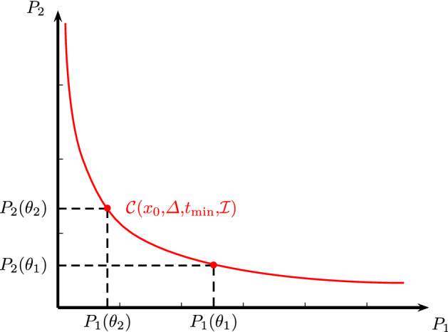
Illustration of a trade-off curve $\mathcal{C}(x_0,\Delta ,t_{\min },\mathcal{I})$ parametrized by thresholds $\theta$ when the number of outcomes is $m=2$

Comparing event-triggered policies based on indicators

To compare the efficiency of two event-triggered feedbacks based on two different epidemiological indicators ${\mathcal{I}}_a$ and ${\mathcal{I}}_b$, we propose to compute the associated trade-off curves described in the previous section. If the policies based on indicators ${\mathcal{I}}_a$ and ${\mathcal{I}}_b$ consider observation time windows ${\Delta }_a$ and ${\Delta }_b$, respectively, and minimum interevent times $t_{\min }^a$ and $t_{\min }^b$, respectively, then we compare the trade-off curves ${\mathcal{C}}_a=\mathcal{C}(x_0,{\Delta }_a,t_{\min }^a,{\mathcal{I}}_a)$ and ${\mathcal{C}}_b=\mathcal{C}(x_0,{\Delta }_b,t_{\min }^b,{\mathcal{I}}_b)$ defined in (6).

Recall that the outcomes are represented by the function $\mathbf{P}:\mathbf{X}\times \mathbb{U}⟶{\mathbb{R}}^m$, with $m\ge 2$, and the aim is to have the m outcomes

$$\begin{array}{c}\hfill \mathbf{P}(x_0,\mathbf{u})=(P_1(x_0,\mathbf{u}),\dots ,P_m(x_0,\mathbf{u}))\end{array}$$

to be as low as possible. Then, the calculation of the trade-off curves ${\mathcal{C}}_a$ and ${\mathcal{C}}_b$, consists of the evaluation of function $\mathbf{P}$ for event-triggered controls ${\mathbf{u}}_a({\theta }_a)=\mathfrak{m}({\Delta }_a,t_{\min }^a,{\mathcal{I}}_a,{\theta }_a)$ and ${\mathbf{u}}_b({\theta }_b)=\mathfrak{m}({\Delta }_b,t_{\min }^b,{\mathcal{I}}_b,{\theta }_b)$ with different values of thresholds ${\theta }_a$ and ${\theta }_b$.

If a decision maker considers as objective (maximal bounds) the first $m-1$ outcomes ${\widehat{\mathbf{P}}}_{1:m-1}=({\widehat{P}}_1,\dots ,{\widehat{P}}_{m-1})$ (e.g., peak demand of ICU beds), the corresponding m-th outcomes $P_m^a$ and $P_m^b$ (e.g., total time of NPI) obtained using event-triggered feedbacks based on indicators ${\mathcal{I}}_a$ and ${\mathcal{I}}_b$ can be computed such that

$$\begin{array}{c}\hfill ({\widehat{\mathbf{P}}}_{1:m-1},P_m^a)\in {\mathcal{C}}_a\text{and}({\widehat{\mathbf{P}}}_{1:m-1},P_m^b)\in {\mathcal{C}}_b.\end{array}$$

Thus, the decision maker should consider the policy based on ${\mathcal{I}}_a$ or ${\mathcal{I}}_b$ comparing $P_m^a$ and $P_m^b$ decision depending on the given objective outcomes ${\widehat{\mathbf{P}}}_{1:m-1}$. In Fig. 2, we show two trade-off curves for $m=2$. In this figure, for small objective values of outcome ${\widehat{P}}_1$, it is better to use a policy based on indicator ${\mathcal{I}}_b$. Otherwise, for larger values of ${\widehat{P}}_1$, it is recommended to use a policy based on ${\mathcal{I}}_a$.

Fig. 2.

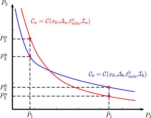
Illustration of the trade-off curves ${\mathcal{C}}_a$ and ${\mathcal{C}}_b$ corresponding to event-triggered feedbacks based on indicators ${\mathcal{I}}_a$ and ${\mathcal{I}}_b$, when the number of outcomes $m=2$ and there is no domination

If $P_m^b<P_m^a$ for all objective outcomes ${\widehat{\mathbf{P}}}_{1:m-1}$, it means that the curve ${\mathcal{C}}_b$ dominates curve ${\mathcal{C}}_a$ and therefore, the policy based on ${\mathcal{I}}_b$ is always better. This situation is illustrated in Fig. 3 for $m=2$.

Fig. 3.

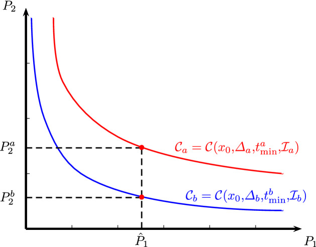
Illustration of trade-off curves ${\mathcal{C}}_a$ and ${\mathcal{C}}_b$ corresponding to event-triggered feedbacks based on indicators ${\mathcal{I}}_a$ and ${\mathcal{I}}_b$, when the number of outcomes is $m=2$ and one curve dominates the other

Finding a control $\mathbf{u}\in \mathbb{U}$ that minimizes the m outcomes given by the vector $\mathbf{P}(x_0,\mathbf{u})=(P_1(x_0,\mathbf{u}),\dots ,P_m(x_0,\mathbf{u}))$ is evidently a multicriteria optimization problem. Therefore, we only propose to compare single outcomes obtained from two policies when the other ($m-1$) outcomes are fixed and treated as objectives. This avoids the need to consider outcomes of different nature and expressed in different units in a single objective function. On the other hand, to compare two policies when several outcomes are simultaneously considered (i.e., not fixed) is technically possibly, although it is not straightforward.

Examples

We present two case studies, one for Chile (Metropolitan Region) and one for China. For both cases we ran simulations in Python based on parameters estimated using Markov chain Monte Carlo for the first example. We refer to “Appendix A” for a description of the calibration algorithm and the parameter priors used in Sect. 4.1 (Chile). For the example in Sect. 4.2 (China), we use the information (model and parameters) provided in the recent publication (Ivorra et al. 2020). The source code, data, and scripts used in both sections are available in https://github.com/COVID19-CMM/jomb-assessment-indicators.

Case study: Metropolitan Region, Chile

For this example, we use a discrete-time compartmental model where the population of Metropolitan Region, Chile (Santiago) $N=7,112,808$ (according to the Chilean Institute of Statistics INE1), assumed to be constant and isolated, is distributed into eight groups corresponding to different disease stages. Susceptible (denoted by $S$) are individuals not infected by the disease but who can be infected by the virus. Exposed (denoted by $E$) are those in the incubation time after being infected. In this stage, they do not have symptoms but can infect other people with a lower probability than those in the infectious group described below. Mild infected or subclinical (denoted by $I^m$) is an infected population that can also infect other people. In this stage, they are asymptomatic or show mild symptoms. They are not detected and thus are not reported by authorities. At the end of this stage, they pass directly to the recovered state. Infected (denoted by $I$) are infected citizens that can infect other people. They develop symptoms and are detected and reported by authorities. They can recover or enter to some hospitalized state. Recovered (denoted by $R$) is a population that survives the illness, is no longer infectious, and has developed immunity to the disease. Hospitalized (denoted by $H$) are patients hospitalized in basic facilities. After this stage, hospitalized can recover or get worse and use an ICU bed or die. Hospitalized in ICU beds (denoted by $H^c$) are patients in critical care. People in these two last stages may infect other people; however, in our posterior analysis, we will neglect this source of infection because we assume that hospitalized individuals are highly isolated. After leaving the ICU bed, they either come back to the basic facilities in the hospital or die. The term dead (denoted by $D$) accounts for people who did not survive the disease.

The evolution of the previous state variables is described by the following discrete-time system, with states $x=(S,E,I^m,I,R,H,H^c,D)\in \mathbf{X}={\mathbb{R}}_{+}^8$:

$$\begin{array}{c}\hfill \left\{\begin{array}{ccc}S(t+1)\hfill & =& S(t)-\Lambda (x(t))S(t)\hfill \\ E(t+1)\hfill & =& E(t)+\Lambda (x(t))S(t)-{\gamma }_{E}E(t)\hfill \\ I^m(t+1)\hfill & =& I^m(t)+(1-{\varphi }_{\mathit{EI}}){\gamma }_{E}E(t)-{\gamma }_{I^m}{I}^m(t)\hfill \\ I(t+1)\hfill & =& I(t)+{\varphi }_{\mathit{EI}}{\gamma }_{E}E(t)-{\gamma }_{I}I(t)\hfill \\ R(t+1)\hfill & =& R(t)+{\gamma }_{I^m}{I}^m(t)+{\varphi }_{\mathit{IR}}{\gamma }_{I}I(t)+{\varphi }_{\mathit{HR}}{\gamma }_{H}H(t)\hfill \\ H(t+1)\hfill & =& H(t)+(1-{\varphi }_{\mathit{IR}}){\gamma }_{I}I(t)+(1-{\varphi }_{H^{c}D}){\gamma }_{H^c}{H}^c(t)-{\gamma }_{H}H(t)\hfill \\ H^c(t+1)\hfill & =& H^c(t)+(1-{\varphi }_{\mathit{HR}}-{\varphi }_{\mathit{HD}}){\gamma }_{H}H(t)-{\gamma }_{H^c}{H}^c(t)\hfill \\ D(t+1)\hfill & =& D(t)+{\varphi }_{\mathit{HD}}{\gamma }_{H}H(t)+{\varphi }_{H^{c}D}{\gamma }_{H^c}{H}^c(t),\hfill \end{array}\right)\end{array}$$ 7

where natural births and deaths are not considered because their effects are negligible.

The above system is a type of discrete-time SEIR (or SEIRHD) model. It aims to better describe an outbreak where part of the population has been infected by a virus, with many people with no symptoms or only mild symptoms. It was found that this is the case for SARS-CoV-2, as has been reported in several papers in the literature (Ferguson et al. 2020; Ivorra et al. 2020; Liu et al. 2020). The model we use can be extended to consider age ranges and evaluate other indicators or policies such as the schools reopening or the progressive lifting of quarantines according to age groups as explored in Zhao et al. (2020) and Zhao and Feng (2020). However, to illustrate the proposed methodology, we have only considered one age class.

The structure of this mathematical model, along with the transitions among the different stages, is shown in Fig. 4.

Fig. 4.

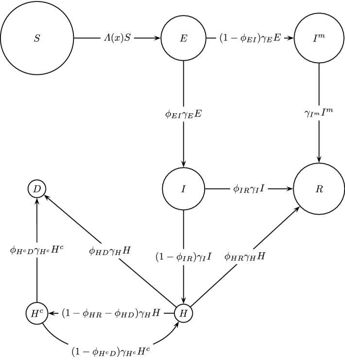
Structure of the mathematical model for the COVID-19 dynamics in an isolated city (Metropolitan Region, Chile). Each circle represents a specific group. Susceptible individuals ($S$), and different disease states: exposed ($E$), mild infected ($I^m$), infected ($I$), recovered ($R$), hospitalized ($H$), hospitalized in ICU beds ($H^c$), and dead ($D$)

We proceed now to describe the main components of system (7). First, we consider the time interval $[[t_0:T]]$, with days as the unit of time, where $t_0$ is the initial time from which we start the assessment of different policies (September 21, 2020) and $T$ is the time horizon. In this example, the time horizon is the simulation time and must be large enough for all of the considered policies (NPI triggered by indicators) to be able to reduce the number of infected people to zero (September 21, 2025), without considering other interventions.

The contagion rate (see the first and second equation in (7)) is

$$\begin{array}{c}\hfill \Lambda (x(t))=\frac{1}{(N-D(t))}({\beta }_{E}E(t)+{\beta }_{I^m}{I}^m(t)+{\beta }_{I}I(t)+{\beta }_{H}H(t)+{\beta }_{H^c}{H}^c(t)),\\ \hfill \end{array}$$ 8

where the specific rates ${\beta }_E,{\beta }_{I^m},{\beta }_I,{\beta }_H,{\beta }_{H^c}$ can be written as the product of the contagion probabilities ($p_E$, $p_{I^m}$, $p_I$, $p_H$, and $p_{H^c}$) and the reference values of contact rates ($c_E^{\mathrm{ref}}$, $c_{I^m}^{\mathrm{ref}}$, $c_I^{\mathrm{ref}}$, $c_H^{\mathrm{ref}}$, and $c_{H^c}^{\mathrm{ref}}$), each value associated with a contagious stage of the disease (indicated in the subindex). Therefore, one has ${\beta }_E=p_E{c}_E^{\mathrm{ref}}$,  ${\beta }_{I^m}=p_{I^m}{c}_{I^m}^{\mathrm{ref}}$,   ${\beta }_I=p_I{c}_I^{\mathrm{ref}}$,   ${\beta }_H=p_H{c}_H^{\mathrm{ref}}$,  and ${\beta }_{H^c}=p_{H^c}{c}_{H^c}^{\mathrm{ref}}$.

The rest of parameters defining dynamics (7), including the initial conditions, are described in “Appendix A” where we explain the calibration procedure for this example.

Basic qualitative analysis

Basic qualitative analysis can be studied through positivity, existence of fixed points and stability.

Positivity: If we assume that the initial states are positive, it is easy to see positive forward invariance; this is, if all components of

$$\begin{array}{c}\hfill x(t)=(S(t),E(t),I^m(t),I(t),R(t),H(t),H^c(t),D(t))\in \mathbf{X}={\mathbb{R}}_{+}^8\end{array}$$

are positive, then all components of $x(t+1)$ are also positive.

This follows from $0<1-{\varphi }_{\mathit{HR}}-{\varphi }_{\mathit{HD}}<1$, $0<{\varphi }_i<1$ and consequently $0<1-{\varphi }_i<1$; and the assumptions that all $0<{\gamma }_i<1$ and thus $0<1-{\gamma }_i<1$ (see “Appendix A”).

Also, from the calibration procedure, we assume that the values of rate parameters ${\beta }_i$ are positive and small enough (less than 1), and thus

$$\begin{array}{cc}& {\beta }_{E}E(t)+{\beta }_{I^m}{I}^m(t)+{\beta }_{I}I(t)+{\beta }_{H}H(t)+{\beta }_{H^c}{H}^c(t)\le \hfill \\ \hfill & \le (max{\beta }_i)(E(t)+I^m(t)+I(t)+H(t)+H^c(t))\le \hfill \\ \hfill & \le (max{\beta }_i)(N-D(t)).\hfill \end{array}$$

Therefore, the contagion rate $\Lambda (x(t))$ defined in (8) satisfies

$$\begin{array}{c}\hfill 0\le \Lambda (x(t))\le max{\beta }_i\le 1,\end{array}$$

and consequently

$$\begin{array}{c}\hfill 0\le 1-\Lambda (x(t))\le 1.\end{array}$$

From the previous inequalities, it easily follows that if all components of the state x(t) are positive, then all components of $x(t+1)$ are positive, and we can conclude forward positivity invariance.

Fixed points: From the first equation in system (7) it is easy to see that the fixed points satisfy $\Lambda (x(t))S=0$. After that, and substituting $\Lambda (x(t))S$ in the next equation, it can be easily concluded that $E(t)=0$, and it follows that also

$$\begin{array}{c}\hfill I^m(t)=I(t)=H(t)=H^c(t)=0\end{array}$$

and thus $\Lambda (x(t))=0$.

Then, for each positive (or zero value) of $S,R$ and $D$ we obtain a fixed point, as expected.

We can conclude that the set of fixed points is part of a 3-dimensional linear manifold. Although this is not the focus in this work, stability and bifurcations can be further studied through Central Manifold Theorem for discrete systems and related mathematical tools (Kuznetsov 1998).

Control and indicators to be used

Our goal is to influence the contagion rate $\Lambda (x(t))$ in (8) with a control policy $u(t)$, representing the application of NPI, in this example, a lockdown, having as effect a reduction in the contact rates. We denote by $\widehat{\Lambda }(x(t),u(t))$ the controlled contagion rate and we define controlled specific contagion rates ${\widehat{\beta }}_E,{\widehat{\beta }}_{I^m},{\widehat{\beta }}_I,{\widehat{\beta }}_H,{\widehat{\beta }}_{H^c}$ as follows

$$\begin{array}{c}\hfill \left\{\begin{array}{ccccc}{\widehat{\beta }}_E(u_E)\hfill & =& (1-u_E){\beta }_E\hfill & =& (1-u_E)p_E{c}_E^{\mathrm{ref}}\hfill \\ {\widehat{\beta }}_{I^m}(u_{I^m})\hfill & =& (1-u_{I^m}){\beta }_{I^m}\hfill & =& (1-u_{I^m})p_{I^m}{c}_{I^m}^{\mathrm{ref}}\hfill \\ {\widehat{\beta }}_I(u_I)\hfill & =& (1-u_I){\beta }_I\hfill & =& (1-u_I)p_I{c}_I^{\mathrm{ref}}\hfill \\ {\widehat{\beta }}_H(u_H)\hfill & =& (1-u_H){\beta }_H\hfill & =& (1-u_H)p_H{c}_H^{\mathrm{ref}}\hfill \\ {\widehat{\beta }}_{H^c}(u_{H^c})\hfill & =& (1-u_{H^c}){\beta }_{H^c}\hfill & =& (1-u_{H^c})p_{H^c}{c}_{H^c}^{\mathrm{ref}}\hfill \end{array}\right)\end{array}$$ 9

where $u=(u_E,u_{I^m},u_I,u_H,u_{H^c})\in {[0,1]}^5$ is the initial vector of control variables that later will be reduced.

We shall assume that $c_H^{\mathrm{ref}}=c_{H^c}^{\mathrm{ref}}=0$ because we suppose that the hospitalized patients are highly isolated. Therefore, $u_H$ and $u_{H^c}$ are no longer considered as control variables. This approach is also used in Koo et al. (2020). Additionally, we assume that the policy for the exposed and mild-infected individuals is the same and thus $u_E=u_{I^m}$, which will be denoted $u$ for simplicity. This means that NPI have the same effects (in terms of the contact rates reduction) for the people in the incubation stage and for the infected population with mild symptoms because these populations are not detected, so that NPI such as lockdowns are assumed to affect them similarly. Finally, we also assume that NPI do not have additional effects in terms of the contact rates reduction, in the infected population with symptoms (and then detected and reported by authorities) because we assume that these individuals are already isolated. Thus, we set $u_I=1-\widehat{\delta }$ with $\widehat{\delta }\in (0,1)$ representing the fraction of nonisolated infected (detected) population. Our vector of control variables is then reduced to a single input $u\in [0,1]$ and the (controlled) contagion rate becomes

$$\begin{array}{c}\hfill \widehat{\Lambda }(x(t),u(t))=\frac{1}{(N-D(t))}\left((1-u(t)),({\beta }_{E}E(t)+{\beta }_{I^m}{I}^m(t)),+,\widehat{\delta },{\beta }_I,I,(t)\right).\end{array}$$ 10

Furthermore, we set $1-\widehat{\delta }$ as the upper bound for the control variable, thus representing that NPI cannot isolate people to a greater extent than the isolation already imposed on the infected and detected population. Therefore, the single control variable $u$ belongs to the control space $\mathbf{U}=[0,1-\widehat{\delta }]$. In the following, we set $\widehat{\delta }=0.2$.

Now we can write the (autonomous) dynamics $f:\mathbf{X}\times \mathbf{U}⟶\mathbf{X}$, where the state space is $\mathbf{X}={\mathbb{R}}_{+}^8$, defining the discrete-time control system of this example as in (1) as follows

$$\begin{array}{c}\hfill \begin{array}{cc}\hfill f(x,u)=f(S,E,I^m,I,R,H,H^c,D,u)& \\ \hfill =\left(\begin{array}{c}S-\widehat{\Lambda }(x,u)S\\ E+\widehat{\Lambda }(x,u)S-{\gamma }_{E}E\\ I^m+(1-{\varphi }_{\mathit{EI}}){\gamma }_{E}E-{\gamma }_{I^m}{I}^m\\ I+{\varphi }_{\mathit{EI}}{\gamma }_{E}E-{\gamma }_{I}I\\ R+{\gamma }_{I^m}{I}^m+{\varphi }_{\mathit{IR}}{\gamma }_{I}I+{\varphi }_{\mathit{HR}}{\gamma }_{H}H\\ H+(1-{\varphi }_{\mathit{IR}}){\gamma }_{I}I+(1-{\varphi }_{H^{c}D}){\gamma }_{H^c}{H}^c-{\gamma }_{H}H\\ H^c+(1-{\varphi }_{\mathit{HR}}-{\varphi }_{\mathit{HD}}){\gamma }_{H}H-{\gamma }_{H^c}{H}^c\\ D+{\varphi }_{\mathit{HD}}{\gamma }_{H}H+{\varphi }_{H^{c}D}{\gamma }_{H^c}{H}^c,\end{array}\right),\end{array}\end{array}$$ 11

where the controlled contagion rate $\widehat{\Lambda }(x,u)$ is given by (10).

Now we describe the elements for defining the event-triggered controls introduced in Sect. 2.2. The considered observation time window and the minimum time of implementation (or minimum interevent time) will be $\Delta =t_{\min }=14$ days. The event-triggering mechanism, as described in (2) and (4), is defined by $u_{\mathrm{ref}}=1-\widehat{\delta }$ (associated with $u(t_0)$ in (2)) and as controllers ${\widehat{u}}_{-},{\widehat{u}}_{+}:[[0:T-t_0]]\times \mathbf{U}⟶\mathbf{U}$ (see (4)), we consider max-linear functions of the form

$$\begin{array}{cc}\hfill {\widehat{u}}_{-}(\tau ,u)=& max\left\{0,,,u,\left(1,-,\frac{\tau }{t_{\min }}\right)\right\}\hfill \\ \hfill {\widehat{u}}_{+}(\tau ,u)=& min\left\{1,-,\widehat{\delta },,,u,\left(1,-,\frac{\tau }{t_{\min }}\right),+,\left(\frac{1-\widehat{\delta }}{t_{\min }}\right),\tau \right\}.\hfill \end{array}$$

These controllers permit to monotonically decrease/increase the strength of the NPI in $t_{\min }$ days until saturating it. We have decided to consider that our control saturates in $t_{\min }$ days, coinciding with the minimum interevent time assuming that at the end of this period of time, the effect of NPI (or their release) is fully accomplished, producing the maximal isolation ($u=1-\widehat{\delta }$) or reaching the normal contact rates equal to those before the pandemic ($u=0$).

To define trigger indicators $\mathcal{I}:{\mathbf{X}}^{\Delta +1}⟶\mathbb{R}$ and then the event-triggered sets $\mathcal{S}$, as in Sect. 3, we consider the following instantaneous observations of the state $\mathcal{O}:\mathbf{X}⟶\mathbb{R}$:

(O1)

Number of hospitalized people in ICU beds:

$$\begin{array}{c}\hfill \mathcal{O}(x(\tau ))=H^c(\tau );\end{array}$$

(O2)

Number of active cases (infectious persons detected) per 100,000 residents:

$$\begin{array}{c}\hfill \mathcal{O}(x(\tau ))=\left(\frac{100,000}{N}\right)(I(\tau )+H(\tau )+H^c(\tau )).\end{array}$$

As established in Sect. 2.2, given an observation time window of $\Delta =14$ days, the indicators to be used are defined for the recent history of the state

$$\begin{array}{c}\hfill {\mathbf{x}}_{\Delta }(t)=(x(t-\Delta ),\dots ,x(t))\in {\mathbf{X}}^{\Delta +1}.\end{array}$$

Thus, the indicators considered in this example are computed from the observations defined in (O1) and (O2) as follows:

1. the mean of instantaneous observations:

   $$\begin{array}{c}\hfill \mathcal{I}(x_{\Delta }(t))=\frac{1}{\Delta +1}\sum _{\tau =t-\Delta }^t\mathcal{O}(x(\tau ));\end{array}$$
2. the mean of differences of instantaneous observations:

   $$\begin{array}{c}\hfill \mathcal{I}(x_{\Delta }(t))=\frac{1}{\Delta +1}\sum _{\tau =t-\Delta +1}^t(\mathcal{O}(x(\tau ))-\mathcal{O}(x(\tau -1)))=\frac{\mathcal{O}(x(t))-\mathcal{O}(x(t-\Delta ))}{\Delta +1}.\end{array}$$

Thus, we will assess four indicators associated with two instantaneous observations (O1) and (O2) and with two different ways to consider them (a) and (b).

Finally, to compare the performance of different event-triggered controls based on the indicators introduced previously (as introduced in Sects. 3.1 and 3.2), we consider two outcomes, that is, the function of outcomes $\mathbf{P}:\mathbf{X}\times \mathbb{U}⟶{\mathbb{R}}^2$ is given by $\mathbf{P}(x_0,\mathbf{u})=(P_1(x_0,\mathbf{u}),P_2(x_0,\mathbf{u}))$, where the event-triggered control $\mathbf{u}$ is defined by $\mathbf{u}=\mathfrak{m}(\Delta ,t_{\min },\mathcal{I},\theta )$, for a given trigger threshold $\theta$, from an initial state $x_0$ at initial time $t_0$. The outcomes considered are:

(P1)

Peak of ICU demand:

$$\begin{array}{c}\hfill P_1(x_0,\mathbf{u})=\underset{t_0\le t\le T+1}{max}{H}^c(t);\end{array}$$

(P2)

Total number of days in lockdown. This is expressed as a percentage (over the total simulation time) and is computed differently depending on whether our NPI is applied at the initial time $t_0$ or not. If the NPI is applied at $t_0$, it is given by

$$\begin{array}{c}\hfill P_2(x_0,\mathbf{u})=\frac{100}{(T-t_0)}\sum _{k=0}^{k_{\mathbf{u}}}(t_{2k+1}-t_{2k})\end{array}$$

otherwise, we have

$$\begin{array}{c}\hfill P_2(x_0,\mathbf{u})=\frac{100}{(T-t_0)}\sum _{k=0}^{k_{\mathbf{u}}}(t_{2k+2}-t_{2k+1}).\end{array}$$

We note that in the above expressions, $k_{\mathbf{u}}$ is the total number of the switches triggered by the policy $\mathbf{u}$.

Numerical results

In this part, we report the numerical results using the introduced discrete-time control model with the four indicators already defined.

For a given event-triggered feedback $\mathbf{u}=\mathfrak{m}(\Delta ,t_{\min },\mathcal{I},\theta )$ we recall the definition of the trade-off curve associated with indicator $\mathcal{I}$, and parametrized by thresholds $\theta$ (see Sect. 3.1)

$$\begin{array}{c}\hfill \mathcal{C}(x_0,\Delta ,t_{\min },\mathcal{I})=\{\mathbf{P}(x_0,\mathbf{u})|\mathbf{u}=\mathfrak{m}(\Delta ,t_{\min },\mathcal{I},\theta );\theta \in {\mathcal{D}}_{\mathcal{I}}\}\subseteq {\mathbb{R}}^2,\end{array}$$

where ${\mathcal{D}}_{\mathcal{I}}\subseteq \mathbb{R}$ is the domain for the thresholds associated with indicator $\mathcal{I}$. For the four indicators considered here (two instantaneous observations (O1) and (O2) and two different ways to consider them (a) and (b)) and the two introduced outcomes (P1) and (P2), the trade-off curves are depicted in Fig. 5.

Fig. 5.

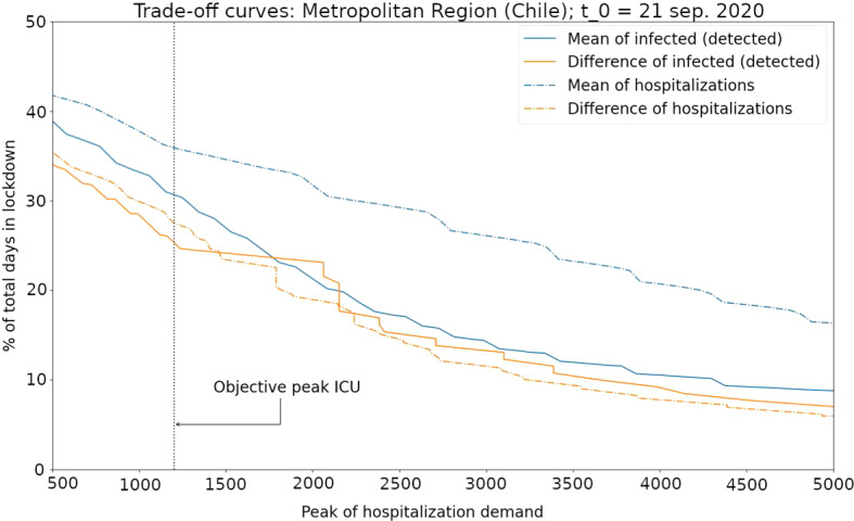
Trade-off curves for the case study of the spread of COVID-19 in Metropolitan Region, Chile. The considered indicators are: number of hospitalized patients in ICU beds (observation (O1)) considering the mean (indicator (a), blue dashed curve) and the mean of difference (indicator (b), orange dashed curve) and the number of active cases (observation (O2)) considering the mean (indicator (a), blue continuous curve) and the mean of difference (indicator (b), orange continuous curve). The curve above the other three curves (indicator (a) using observation (O1), in blue dashed curve) suggests that this indicator is the worst for triggering decisions about NPI (implement/release). For the targeted objective (to have a ICU peak demand at most 1200 beds) the best indicator is the curve crossing at the minimum level (percentage of days in lockdown) the vertical line representengin the target

It is observed from Fig. 5 that the performance of the indicator corresponding to the mean of hospitalized patients in ICU beds (observation (O1) considered as  (a)), depicted by a blue dashed curve, is the worst in comparison to the other indicators in the sense that its trade-off curve is above the other curves; therefore, for any objective in the peak of ICU demand (outcome (P1)), the use of this indicator will imply more days in the lockdown (outcome (P2)). The trade-off curves of the other three indicators are quite similar. Nevertheless, the indicators based in the number of active cases (based in observation  (O2), depicted by continuous curves) in practice can be less reliable that the indicator corresponding to the mean of the difference of the hospitalized patients in ICU beds (based in observation (O1) considered as  (b)) that is shown by the orange dashed curve.

In Table 1, we present the associated threshold for each indicator, having as objective a peak of ICU demand of $P_1(x_0,\mathbf{u})=1,200$ beds (see (P1)). This value corresponds to an approximation of the total ICU beds available during October 2020 for the Metropolitan Region according to Chilean official data (Chilean Ministry of Science, Technology, Knowledge and Innovation 2020). In this table, we also show the percentage of days in lockdown $P_2(x_0,\mathbf{u})$ (see (P2)) associated with each indicators for the objective mentioned above.

Table 1.

Thresholds and percentages of days in lockdown $P_2(x_0,\mathbf{u})$ (see (P2)) associated with four assessed indicators, considering a peak of ICU demand objective of $P_1(x_0,\mathbf{u})=1,200$ beds (see (P1)), in Metropolitan Region (Chile)

Indicator	Threshold	% in lockdown
$\mathcal{I}$	$\theta$	$P_2(x_0,\mathbf{u})$
Mean of ICU (O1); (a)	253	36%
Difference of ICU (O1); (b)	8.9	27%
Mean of active cases (O2); (a)	87	31%
Difference of active cases (O2); (b)	2.2	26%

Case study: China

In this example, we consider the compartmental model published in Ivorra et al. (2020) for the spread of COVID-19 in China. The model is composed by nine state variables corresponding to different stages of the disease: susceptible (S), exposed (E), infectious (I), infectious but undetected ($I_u$), hospitalized that will recover ($H_R$), hospitalized that will die ($H_D$), recovered after being detected ($R_d$), and recovered after being infectious but undetected ($R_u$), and dead by COVID-19 (D). Thus, the vector of the state variables is

$$\begin{array}{c}\hfill x(t)=(S(t),E(t),I(t),I_u(t),H_R(t),H_D(t),R_d(t),R_u(t),D(t))\in \mathbf{X}={\mathbb{R}}_{+}^9.\end{array}$$

Since the model in Ivorra et al. (2020) is established in continuous-time, we consider a very small time step (one hour). Then, we use the standard Euler method to discretize the dynamics in Ivorra et al. (2020) with a step $\Delta t=1/24$ to obtain $f:\mathbf{X}\times \mathbf{U}⟶\mathbf{X}$ as in (1). Thus, for this case-study, the (autonomous) dynamics that define the discrete-time control systems are described by the following:

$$\begin{array}{c}\hfill \begin{array}{cc}\hfill f(x,u)=f(S,E,I,I_u,H_R,H_D,R_d,R_u,D,u)=& \\ \hfill \left(\begin{array}{c}S-\Delta t\widehat{\Lambda }(x,u)S\\ E+\Delta t\left(\widehat{\Lambda },(x,u),S,-,{\gamma }_E,E\right)\\ I+\Delta t\left({\gamma }_E,E,-,{\gamma }_I,I\right)\\ I_u+\Delta t\left((1-{\varphi }_{I{H}_R}-{\varphi }_{I{H}_D}),{\gamma }_I,I,-,{\gamma }_{I_u},I_u\right)\\ H_R+\Delta t\left({\varphi }_{I{H}_R},{\gamma }_I,I,-,{\gamma }_{H_R},H_R\right)\\ H_D+\Delta t\left({\varphi }_{I{H}_D},{\gamma }_I,I,-,{\gamma }_{H_D},H_D\right)\\ R_d+\Delta t{\gamma }_{H_R}{H}_R\\ R_u+\Delta t{\gamma }_{I_u}{I}_u\\ D+\Delta t{\gamma }_{H_D}{H}_D\end{array}\right).\end{array}\end{array}$$ 12

Here, the controlled contagion rate $\widehat{\Lambda }(x,u)$ is given by

$$\begin{array}{c}\hfill \widehat{\Lambda }(x(t),u(t))=\frac{1}{N}(1-u(t))({\beta }_{E}E(t)+{\beta }_{I}I(t)+{\beta }_{I_u}{I}_u(t)+{\beta }_{H_R}{H}_R(t)+{\beta }_{H_D}{H}_D(t)),\\ \hfill \end{array}$$ 13

where a single control variable $u\in \mathbf{U}=[0,1-\widehat{\delta }]$ has been considered. This control is associated with the implementation of NPIs such as lockdowns. It multiplies all of the contagion rates (${\beta }_E$, ${\beta }_I$, ${\beta }_{I_u}$, ${\beta }_{H_R}$ and ${\beta }_{H_D}$), because its main effect is to reduce the contact rates among all individuals. Parameter $\widehat{\delta }\in (0,1)$ represents the fraction of the population that reduces their contact rates during a lockdown (or more generally the application of a given NPI). The latter is considered to be different from zero because, even during lockdowns, some basic services must still operate. In the following, we set $\widehat{\delta }=0.25$.

The parameters defining the dynamics $f:\mathbf{X}\times \mathbf{U}⟶\mathbf{X}$ in (12) are given by the vector $(\beta ,\gamma ,\varphi )\in {\mathbb{R}}_{+}^5\times {\mathbb{R}}_{+}^5\times {[0,1]}^2$. Vector $\beta =({\beta }_E,{\beta }_I,{\beta }_{I_u},{\beta }_{H_R},{\beta }_{H_D})\in {\mathbb{R}}_{+}^5$ contains all of the specific rates associated with the contagious stages of the disease. Parameters $\gamma =({\gamma }_E,{\gamma }_I,{\gamma }_{I_u},{\gamma }_{H_R},{\gamma }_{H_D})\in {\mathbb{R}}_{+}^5$ are the mean rates of the transition from these respective stages to the subsequent stage. In other words, for a disease stage $X\in \{E,I,I_u,H_R,H_D\}$ parameter ${\gamma }_X^{-1}$ days represents the mean duration of stage X. Finally, the vector $\varphi =({\varphi }_{I{H}_R},{\varphi }_{I{H}_D})\in {[0,1]}^2$ allows us to describe the distribution from infected people ($I$) to the next three stages: infected but undetected ($I_u$), hospitalized that will recover ($H_R$), and hospitalized that will die ($H_D$). Indeed, the fraction of infected people that are not detected is given by $1-{\varphi }_{I{H}_R}-{\varphi }_{I{H}_D}$, while ${\varphi }_{I{H}_R}$ and ${\varphi }_{I{H}_D}$ represent the fraction passing from infected to the hospitalized stages $H_R$ and $H_D$, respectively. We note that in Ivorra et al. (2020), both fractions are equivalently written in terms of the case fatality ratio and of the fraction of infected people that are detected. The values of $(\beta ,\gamma ,\varphi )$ used in our simulations correspond to those used in Ivorra et al. (2020) for experiment ${\mathbf{EXP}}_{\mathbf{29}\mathbf{M}}$; see Table 3 in Ivorra et al. (2020).

Additionally, the initial conditions

$$\begin{array}{cc}\hfill x(t_0)& =(S_0,E_0,I_0,{I_u}_0,{H_R}_0,{H_D}_0,{R_d}_0,{R_u}_0,D_0)\in \mathbf{X}={\mathbb{R}}_{+}^9\hfill \end{array}$$

were obtained from the calibration realized with the complete set of data available in Ivorra et al. (2020), that is, our initial condition vector $x(t_0)$ corresponds to the last day output (March 29, 2020) of the fitted model in Ivorra et al. (2020) for experiment ${\mathbf{EXP}}_{\mathbf{29}\mathbf{M}}$. These values are given in Table 2.

Table 2.

Initial conditions for example in Sect. 4.2 corresponding to China, estimated at $t_0=$ March 29, 2020

State variable	Value
$S_0$	1,389,828,000
$E_0$	14
$I_0$	2
${I_u}_0$	1,555
${H_R}_0$	2,035
${H_D}_0$	270
${R_d}_0$	73,622
${R_u}_0$	90,346
$D_0$	3,708

It is important to note that a very strict lockdown was considered in the experiment ${\mathbf{EXP}}_{\mathbf{29}\mathbf{M}}$ in Ivorra et al. (2020). This explains the very low values obtained for the infected stages in Table 2. Recall that our initial time ($t_0=$ March 29, 2020) corresponds to the final time in that experiment after the application of the lockdowns.

Regarding the other elements necessary to pursue our analysis, the event-triggered controls introduced in Sect. 2.2 are defined similarly to those in Sect. 4.1. Indeed, the considered observation time window and the minimal time of implementation (or minimal interevent time) will be $\Delta =t_{\min }=14$ days. The event-triggering mechanism described in (2) and (4) is defined by $u_{\mathrm{ref}}=1-\widehat{\delta }$ (associated with $u(t_0)$ in (2)) and by controllers ${\widehat{u}}_{-},{\widehat{u}}_{+}:[[0:T-t_0]]\times \mathbf{U}⟶\mathbf{U}$ (see (4)) that are considered as max-linear functions of the form

$$\begin{array}{cc}\hfill {\widehat{u}}_{-}(\tau ,u)=& max\left\{0,,,u,\left(1,-,\frac{\tau }{t_{\min }}\right)\right\}\hfill \\ \hfill {\widehat{u}}_{+}(\tau ,u)=& min\left\{1,-,\widehat{\delta },,,u,\left(1,-,\frac{\tau }{t_{\min }}\right),+,\left(\frac{1-\widehat{\delta }}{t_{\min }}\right),\tau \right\}.\hfill \end{array}$$

As in the previous case-study analyzed in Sect. 4.1, our control saturates in $t_{\min }$ days, coinciding with the minimum interevent time. Thus, we assume that at the end of this period of time, the effect of NPI (or their release) is fully accomplished, producing maximal isolation ($u=1-\widehat{\delta }$) or reaching the normal contact rates equal to those prior to the pandemic ($u=0$).

To define trigger indicators $\mathcal{I}:{\mathbf{X}}^{\Delta +1}⟶\mathbb{R}$ and then the event-triggered sets $\mathcal{S}$ (cf. Sect. 3), we also consider the following instantaneous observations of the state:

($\tilde{O}1$)

Number of hospitalized people:

$$\begin{array}{c}\hfill \mathcal{O}(x(\tau ))=H_R(\tau )+H_D(\tau );\end{array}$$

($\tilde{O}2$)

Number of detected infectious people:

$$\begin{array}{c}\hfill \mathcal{O}(x(\tau ))=I(\tau ).\end{array}$$

As established in Sect. 2.2, given an observation time window of 14 days (i.e., $\Delta =14$), the indicators to be used are defined for the recent history of the state

$$\begin{array}{c}\hfill {\mathbf{x}}_{\Delta }(t)=(x(t-\Delta ),\dots ,x(t))\in {\mathbf{X}}^{\Delta +1}.\end{array}$$

Thus, the indicators considered in this case-study are computed from observations defined in ($\tilde{O}1$) and ($\tilde{O}2$) as follows:

1. the mean of instantaneous observations:

   $$\begin{array}{c}\hfill \mathcal{I}(x_{\Delta }(t))=\frac{1}{\Delta +1}\sum _{\tau =t-\Delta }^t\mathcal{O}(x(\tau ));\end{array}$$
2. the mean of differences of instantaneous observations:

   $$\begin{array}{c}\hfill \mathcal{I}(x_{\Delta }(t))=\frac{1}{\Delta +1}\sum _{\tau =t-\Delta +1}^t(\mathcal{O}(x(\tau ))-\mathcal{O}(x(\tau -1)))=\frac{\mathcal{O}(x(t))-\mathcal{O}(x(t-\Delta ))}{\Delta +1}.\end{array}$$

Finally, for the assessment of the different event-triggered controls policies based on the indicators above, we apply the methodology described in Sects. 3.1 and 3.2. Thus, we consider the function of outcomes $\mathbf{P}:\mathbf{X}\times \mathbb{U}⟶{\mathbb{R}}^2$ given by $\mathbf{P}(x_0,\mathbf{u})=({\tilde{P}}_1(x_0,\mathbf{u}),{\tilde{P}}_2(x_0,\mathbf{u}))$, where the event-triggered control $\mathbf{u}$ is defined by $\mathbf{u}=\mathfrak{m}(\Delta ,t_{\min },\mathcal{I},\theta )$ (for a given trigger threshold $\theta$, from an initial state $x_0$ at initial time $t_0$), and the outcomes ${\tilde{P}}_1(x_0,\mathbf{u})$ and ${\tilde{P}}_2(x_0,\mathbf{u})$ are given by the following:

($\tilde{P}1$)

Peak of hospitalization demand:

$$\begin{array}{c}\hfill {\tilde{P}}_1(x_0,\mathbf{u})=\underset{t_0\le t\le T+1}{max}(H_R^{\mathbf{u}}(t)+H_D^{\mathbf{u}}(t)),\end{array}$$

where $H_R^{\mathbf{u}}(t)+H_D^{\mathbf{u}}(t)$ corresponds to the total number of hospitalized patients at period t.

($\tilde{P}2$)

Total number of days of lockdown: This outcome was already defined in Sect. 4.1, outcome (P2). For the sake of completeness, we recall its computation here: If the NPI is applied at $t_0$, it reads as follows

$$\begin{array}{c}\hfill {\tilde{P}}_2(x_0,\mathbf{u})=\frac{100}{(T-t_0)}\sum _{k=0}^{k_{\mathbf{u}}}(t_{2k+1}-t_{2k})\end{array}$$

otherwise, we have

$$\begin{array}{c}\hfill {\tilde{P}}_2(x_0,\mathbf{u})=\frac{100}{(T-t_0)}\sum _{k=0}^{k_{\mathbf{u}}}(t_{2k+2}-t_{2k+1}).\end{array}$$

We note that in the previous expressions, $k_{\mathbf{u}}$ is the total number of the switches triggered by the policy $\mathbf{u}$.

Numerical results

Finally, we report the numerical results for this case study considering the four indicators (two instantaneous observations ($\tilde{O}1$) and ($\tilde{O}2$) and two different ways to consider them (a) and (b)) defined above, consisting in computing their trade-off curves (see Sect. 3.1) given by

$$\begin{array}{c}\hfill \mathcal{C}(x_0,\Delta ,t_{\min },\mathcal{I})=\{\mathbf{P}(x_0,\mathbf{u})|\mathbf{u}=\mathfrak{m}(\Delta ,t_{\min },\mathcal{I},\theta );\theta \in {\mathcal{D}}_{\mathcal{I}}\}\subseteq {\mathbb{R}}^2.\end{array}$$

The four trade-off curves are depicted in Fig. 6.

Fig. 6.

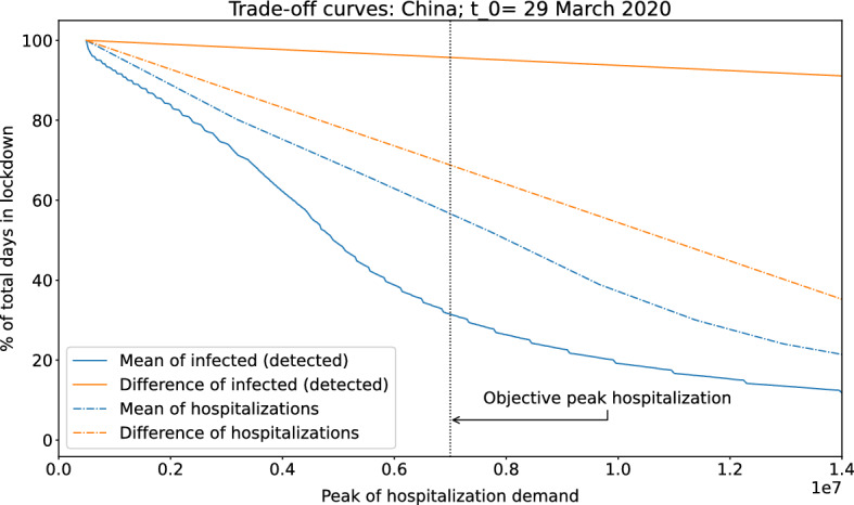
Trade-off curve for our case-study based on the spread of COVID-19 in China. Four indicators are considered: number of hospitalized people (observation ($\tilde{O}1$)) considering the mean (indicator (a), blue dashed curve) and the mean of difference (indicator (b), orange dashed curve) and the number of active cases (observation ($\tilde{O}2$)) considering the mean (indicator (a), blue continuous curve) and the mean of difference (indicator (b), orange continuous curve). The curve below the other three curves (indicator (a) using observation ($\tilde{O}2$), in blue continuous curve) suggests that this indicator is the best for triggering decisions about NPI (implement/release) because for any targeted objective (to have a maximal hospital demand) the percentage of days in lockdown using this indicator is lower

Figure 6 shows that the 14-day rolling average of infected and detected people (observation ($\tilde{O}2$) considered as  (a)) is clearly the best indicator among the four analyzed indicators. The second best indicator is the mean of total hospitalizations due to COVID-19 (observation ($\tilde{O}1$) considered as  (a)), but its performance is considerably weaker. For instance, when we consider an objective peak hospitalization demand of 7 million of beds (that is, ${\tilde{P}}_1(x_0,\mathbf{u})=7,000,000$; see outcome ($\tilde{P}1$)), the percentage of time in lockdowns (outcome ($\tilde{P}2$)) for the policies associated with each indicator is given by ${\tilde{P}}_2(x_0,\mathbf{u})=$ 31% and 57%, respectively, over the total analyzed time. This demonstrates the strong advantage of using a policy associated with the rolling average of infected people with respect to the other analyzed indicators in this case. Therefore, our analysis suggest the use of this indicator as the basis for an event-triggered policy for this case study.

In Table 3 we show the percentage of the days in lockdown ${\tilde{P}}_2(x_0,\mathbf{u})$ (see ($\tilde{P}2$)) associated with each indicator when the objective peak hospitalization demand is ${\tilde{P}}_1(x_0,\mathbf{u})=7,000,000$ beds (see ($\tilde{P}1$)). We also present the associated thresholds $\theta$ for these four indicators.

Table 3.

Thresholds and percentages of days in lockdown ${\tilde{P}}_2(x_0,\mathbf{u})$ (see ($\tilde{P}2$)) associated with the four assessed indicators considering the peak hospitalization demand of ${\tilde{P}}_1(x_0,\mathbf{u})=7,000,000$ beds (see ($\tilde{P}1$)) in China as the objective

Indicator	Threshold	% in lockdown
$\mathcal{I}$	$\theta$	${\tilde{P}}_2(x_0,\mathbf{u})$
Mean of hospitalized people ($\tilde{O}1$); (a)	295,926	57%
Difference of hospitalized people ($\tilde{O}1$); (b)	– 1,137	69%
Mean of detected infectious people  ($\tilde{O}2$); (a)	3,932,230	31 %
Difference of detected infectious people ($\tilde{O}2$); (b)	– 6,607	96 %

Final remarks

In this work, we addressed two main goals: to propose a modeling framework for representing the decision-making process related to the application of NPI policies based on the observation of epidemiological indicators and to introduce a methodology to compare the effectiveness of these strategies (defined by trigger indicators) with respect to multiple objectives outcomes. The proposed framework is that of event-triggered controls with some specific details such as considering the state in a window of time and imposing a minimum intervention time (or minimum interevent time). Both features were introduced in order to represent the application of the NPIs more realistically.

The two case-studies discussed in Sect. 4 show how our methodology can be used to recommend an indicator-based policy when some given outcomes are treated as objectives in our analysis. Nevertheless, our approach should be consider only as a guide to suggest a recommendation. In practice, decision makers must also undertake a complementary and more in-depth analysis. For instance, the observability of the indicators under analysis is something that must also be taken into account. Indeed, when an indicator based on active cases has a similar performance to that of another indicator based, for instance, on the number of hospitalized patients (as in the case-study given in Sect. 4.1), a possible recommendation is to consider a policy based on the second type of indicator because the corresponding observations (hospitalized patients) are more reliable and, consequently, the latter is a more robust NPI policy in practice.

As described in this article, our approach permits to represent the decision-making process based on the observation of indicators and compare the use of these indicators to define NPI policies from a cost-benefit perspective. This comparison will depend on the outcomes chosen as objectives and also on the structure of the dynamic model and on the indicators chosen for this comparison. Both of the latter mathematical objects are intrinsically related in the sense that the dynamics considered as a basis in our methodology must allow the computation and simulation of the indicators that we seek to compare in the analysis. Therefore, for assessment of more elaborate indicators such as positivity rates, indicators associated with testing and contact tracing and effective reproduction number, it is necessary to consider dynamical systems with compartmental stages that allows the formulation of such indicators. On the other hand, our methodology was demonstrated for two SEIR-type models that are some of the most common mathematical models in epidemiology. Nevertheless, our methodology can also be adapted to other underlying mathematical models, such as agent-based models. Of course, different dynamics or other underlying mathematical models can lead to different recommendations. However, this issue is inherent to any real-life decision derived from a mathematical analysis.

It should be noted that this research was carried out when no pharmacological interventions were available, so the underlying models in the case studies presented in this paper do not consider the effects of vaccines on disease progression. However, the methodology introduced can be implemented with models where the effects of pharmacological interventions are considered, such as those developed in Buonomo (2020) and Ramos et al. (2021), and in situations where the implementation and lifting of NPIs is still the subject of public policy.

The framework introduced in this paper for assessing indicators-based event-triggered policies raises some interesting problems to study the further theoretical analysis of which can have important repercussions on the decision-making process. We mention three such problems:

• Time consistency: When the analysis introduced in Sect. 3.2 for determining the best indicator to use is carried out at time $t_0$, following the policy induced by this indicator, there is no guarantee that this strategy will be the best in the long term. Since the trade-off curves are dynamic objects because they depend on the initial conditions (see (6)), it is possible that with time, another indicator should be chosen for triggering NPIs, because its performance is better considering the future state as the initial condition.

  In the terms of trade-off curves and the comparison process proposed in Sect. 3.2, the aforementioned situation occurs when two of these curves (the best chosen at $t_0$ and other), viewed as curves that evolve in time, intersect in a future time at the level (in the outcomes space) corresponding to the $m-1$ outcomes objectives for which the analysis was carried out at time $t_0$. To prove that a future intersection between the trade-off curves will not occur will clearly require to assume certain properties of the dynamics and the compared indicators; this is an interesting problem. A similar problem in the context of linear system where the performance (i.e., our outcomes) is a quadratic cost, is studied in Antunes and Khashooei (2016).

  On the other hand, it is natural to consider situations where the outcomes objectives can evolve in time. For instance, at time $t_0$ the situation is analyzed considering a given ICU maximal capacity but perhaps in some months, this capacity will be increased. In summary, the comparison process of indicators-based event-triggered policies should be implemented continuously across the evolution of the disease in the population, taking into account eventual updating of objective outcomes by the decision makers. Due the latter and the dynamics aspect of trade-off curves, with longer time it is possible that a discarded indicator will in fact become the best indicator.

• Is it better to consider policies based on more indicators? In the analysis proposed in this work, we have considered only policies based on a single indicator. That is, to consider event-triggered sets $\mathcal{S}$, defined in the space of the recent history of states ${\mathbf{X}}^{\Delta +1}$, in the form

  $$\begin{array}{c}\hfill \mathcal{S}=\mathcal{S}(\Delta ,\mathcal{I},\theta )=\{{\mathbf{x}}_{\Delta }\in {\mathbf{X}}^{\Delta +1}|\mathcal{I}({\mathbf{x}}_{\Delta })\le \theta \},\end{array}$$ 14

  where the indicator $\mathcal{I}:{\mathbf{X}}^{\Delta +1}⟶\mathbb{R}$ takes values in $\mathbb{R}$ and $\theta \in \mathbb{R}$ is a threshold for this indicator. Consideration of more indicators leads to the consideration of a vector-valued function $\mathcal{I}:{\mathbf{X}}^{\Delta +1}⟶{\mathbb{R}}^p$, with $p\ge 2$, and the inequality $\mathcal{I}({\mathbf{x}}_{\Delta })\le \theta$ in (14) with respect to the componentwise order for a vector of thresholds $\theta \in {\mathbb{R}}^p$. We wonder if the question of whether more indicators lead to better policies can be formulate as follows: If $\mathcal{S}(\mathcal{I},\theta )\subseteq \mathcal{S}(\tilde{\mathcal{I}},\theta )$ for all vector of threshold $\theta$ (in an appropriate domain) can one conclude that a policy based on $\mathcal{I}$ is better than one based on $\tilde{\mathcal{I}}$ (or vice versa)?

  For triggering NPIs it can be natural to consider various indicators, as in the examples cited in the introductory section, motivated by the reliability (or the lack of) of observations for making decisions. Nevertheless, assuming that all observations are reliables, it is not clear that the addition of indicators for triggering the decisions will induce better policies from the cost-effectiveness viewpoint.

• Stochastic analysis: The framework introduced in this work can be extended considering stochastic dynamics and indicators. In this case, a possible additional outcome that can be considered is the maximum probability of satisfying the other outcomes (seen as objectives), and then the performance of different event-triggered policies can be assessed in terms of that probability, considering the risk-aversion of the decision makers.

  To considering stochastic dynamics, the estimated probabilities distributions of involved parameters can be take as one of the output given by the calibration procedure used in Sect. 4.1 and mentioned in “Appendix A”.

Perhaps using simple models (few state variables) it is possible to provide mathematical proofs for the questions posed in the first two points of the previous list, that is, to ensure that the trade-off curves do not intersect in the future and to deduce when an indicator is better than others from the properties of the event-triggered sets $\mathcal{S}$ corresponding to those indicators. Eventually the theoretical analysis can be simpler considering feedbacks based only on the instantaneous observations and time-continuous dynamics, a framework have purposefully avoided here because the measurability of the involved functions merits a deeper analysis. The aforementioned problems are beyond the scope of this paper; however, we plan to study them in future works.

Parameter description and calibration procedure of model in Sect. 4.1

The parameters of system (7) associated with dynamics $f:\mathbf{X}\times \mathbf{U}⟶\mathbf{X}$ given by (11) are contained in the vector $(\beta ,\gamma ,\varphi )\in {\mathbb{R}}_{+}^3\times {\mathbb{R}}_{+}^5\times {[0,1]}^5$, where $\beta =({\beta }_E,{\beta }_{I^m},{\beta }_I)\in {\mathbb{R}}_{+}^3$ is the vector of the specific rates associated with contagious stages of the disease and that are involved in the definition of the controlled contagion rate $\widehat{\Lambda }(x(t),u(t))$ given by (10).

Parameters $\gamma =({\gamma }_E,{\gamma }_{I^m},{\gamma }_I,{\gamma }_H,{\gamma }_{H^c})\in {\mathbb{R}}_{+}^5$ are the mean rates of transition from the respective stages to the next stage. In other words, for a disease stage $X\in \{E,I^m,I,H,H^c\}$ parameter ${\gamma }_X^{-1}$ days represents the mean duration of stage X.

The vector $\varphi =({\varphi }_{\mathit{EI}},{\varphi }_{\mathit{IR}},{\varphi }_{\mathit{HR}},{\varphi }_{\mathit{HD}},{\varphi }_{H^{c}D})\in {[0,1]}^5$ contains different distribution fractions between the different stages. Thus, ${\varphi }_{\mathit{EI}}$ is the fraction of exposed people who become infected (with symptoms), ${\varphi }_{\mathit{IR}}$ is the fraction of infected people who recover, ${\varphi }_{\mathit{HR}}$ is the fraction of hospitalized (in normal services) people who recover, ${\varphi }_{\mathit{HD}}$ is the fraction of hospitalized (in normal services) people who die, and ${\varphi }_{H^{c}D}$ is the fraction of hospitalized people in ICU beds who die.

The parameters have been estimated using a Hamiltonian Markov chain Monte Carlo estimation method using the Stan library (Carpenter et al. 2017). The method is a Bayesian approach that allows the approximation of the probability densities for each of the parameters in the system when using a sufficient number of iterations. We use the Gelman-Rubin ($\widehat{R}$) convergence diagnostic and 12 parallel chains to ensure that the separate chains converge to the same values. $\widehat{R}$ compares the variance of each chain to the pooled variance of all chains. Each of the parameters obtained an $\widehat{R}\le 1.03$ where each chain ran 10,000 iterations of which a half were warm-up.

For each of the parameters, we set upper and lower limits to restrict the parameter search space to allow realistic combinations only. In addition, we used a weakly informative prior for each of the parameters with mean values obtained from the literature and broad standard deviations.

In Table 4, we state for each parameter its limits, prior probability distribution in the form of a mean and standard deviation, and some references for the mean of the used prior distributions. The model was trained on data from June 20, 2020, until September 20, 2020, in the Metropolitan Region (Chile), considering the total number of COVID-19 cases (symptomatic), the number of patients in ICU, and the number of deceased, according the information collected and published by the Chilean Ministry of Science, Technology, Knowledge and Innovation in (2020). We assume an independent and identically distributed (i.i.d.) error of $\sigma$ for all data points.

Table 4.

Parameter limits, priors, and mean and standard deviation following MCMC estimation

Parameter	Limits	Prior	Value	Reference (mean prior)
${\beta }_E$	[0.002, 0.2]	$\mathcal{N}(0.016,0.1)$	$0.04\pm 3.3\times {10}^{-5}$	–
${\beta }_{I^m}$	[0.002, 0.2]	$\mathcal{N}(0.016,0.1)$	$0.04\pm 3.3\times {10}^{-5}$	–
${\beta }_I$	[0.01, 1]	$\mathcal{N}(0.08,0.5)$	$0.2\pm 1.7\times {10}^{-4}$	–
${\gamma }_E$	[1/15, 1/2]	$\mathcal{N}(1/5.8,0.07)$	$0.39\pm 3.9\times {10}^{-4}$	McAloon et al. (2020)
${\gamma }_{I^m}$	[1/30, 1/5]	$\mathcal{N}(1/9.5,0.07)$	$0.17\pm 1.2\times {10}^{-4}$	Byrne et al. (2020)
${\gamma }_I$	[1/30, 1/5]	$\mathcal{N}(1/7,0.07)$	$0.17\pm 1.4\times {10}^{-4}$	Wang et al. (2020)
${\gamma }_H$	[1/30, 1/5]	$\mathcal{N}(1/11,0.07)$	$0.17\pm 1.1\times {10}^{-4}$	Zhou et al. (2020)
${\gamma }_{H^c}$	[1/30, 1/5]	$\mathcal{N}(1/8,0.07)$	$0.14\pm 1.1\times {10}^{-4}$	Zhou et al. (2020)
${\varphi }_{\mathit{IR}}$	[0.5, 0.99]	$\mathcal{N}(0.7395,0.5)$	$0.61\pm 3.2\times {10}^{-4}$	Centers for Disease Control and Prevention (2020b)
${\varphi }_{\mathit{HR}}$	[0.5, 0.99]	$\mathcal{N}(0.6585,0.5)$	$0.61\pm 3\times {10}^{-4}$	Wang et al. (2020)
${\varphi }_{\mathit{HD}}$	$[0.01,min\{0.5,1-{\varphi }_{\mathit{HR}}\}]$	$\mathcal{N}(0.0244,0.5)$	$0.12\pm 1.5\times {10}^{-4}$	Wang et al. (2020)
${\varphi }_{H^{c}D}$	[0.01, 0.5]	$\mathcal{N}(0.385,0.5)$	$0.12\pm 4.1\times {10}^{-4}$	Huang et al. (2020)
$\sigma$	[0.0, 1.0]	$\mathrm{Cauchy}(0,1)$	$0.02\pm 3\times {10}^{-6}$	–

Since there are no data available of the asymptomatic population, we are not able to train the trajectory of asymptomatic cases from $E$ to $I^m$ and to $R$. That is, the parameters ${\varphi }_{\mathit{EI}}$ and ${\gamma }_{I^m}$ are not trained by maximizing the posterior, except for the small influence through ${\beta }_{I^m}$ that is difficult to distinguish from the other sources of contagion. To mitigate this, we will fix ${\varphi }_{\mathit{EI}}=0.6$ where we assume 60% of the infections to be symptomatic, following Oran and Topol (2020) and Centers for Disease Control and Prevention (2020a, Scenario 5: Current Best Estimate).

The initial conditions $x(t_0)=(S_0,E_0,I_0^m,I_0,R_0,H_0,H_0^c,D_0)\in \mathbf{X}={\mathbb{R}}_{+}^8$, have been estimated using weakly informative priors where we take $E_0$, $I_0^m$, $I_0$, and $H_0$ to have scaled Beta priors between 0 and N with $\alpha =1$ and $\beta =4$ (parameters of Beta distribution), where $N=7,112,808$ is the total population. For the initial number of hospitalized patients in ICU, deceased patients, and total number of infections to date we assume a lognormal distribution with a standard deviation of $\sigma$ around the data. In this setup, $S_0$ and $R_0$ are free variable but we need to restrict at least one of these variables to solve the system. We propose a rough estimate of $R_0$ to be the total number of infected patients to date plus the percentage that were mildly infected. Here, we assume that the number of people that are currently infected, hospitalized, or deceased are small relative to the total population. $S_0$ then follows from $S_0=N-E_0-I_0^m-I_0-H_0-H_0^c-R_0-D_0$. The obtained values of initial conditions are shown in Table 5.

Table 5.

Initial conditions for example in Sect. 4.1 corresponding to Metropolitan Region (Chile), estimated at $t_0=$ September 21, 2020

State	Initial condition
$S_0$	6,671,557
$E_0$	1,697
$I_0^m$	1,723
$I_0$	2,540
$H_0$	1,157
$H_0^c$	433
$R_0$	421,948
$D_0$	11,753

Declarations

Conflict of interest

The authors declare that they have no conflict of interest.

References

- Aba Oud MA, Ali A, Alrabaiah H, Ullah S, Khan MA, Islam S (2021) A fractional order mathematical model for COVID-19 dynamics with quarantine, isolation, and environmental viral load. Adv Differ Equ 19. 10.1186/s13662-021-03265-4 (Paper No. 106) [DOI] [PMC free article] [PubMed]
- Aguilera X, Araos R. Ferreccio C, Otaiza F, Valdivia G, Valenzuela MT, Vial P, O’Ryan M (2020) Consejo Asesor COVID-19 Chile. https://drive.google.com/file/d/1cX3CPnv_3prZGKZF9eTLQsnPInfuw6sE/view (29 Junio 2020)
- Aguilera X, Mundt AP, Araos R, Weitzel T (2021) The story behind Chile’s rapid rollout of COVID-19 vaccination. Travel Med Infect Dis [DOI] [PMC free article] [PubMed]
- Alvarez F, Argente D, Lippi F (2020) A simple planning problem for COVID-19 lockdown. Tech rep. 10.2139/ssrn.3569911
- Alvi MM, Sivasankaran S, Singh M. Pharmacological and non-pharmacological efforts at prevention, mitigation, and treatment for COVID-19. J Drug Target. 2020;28(7–8):742–754. doi: 10.1080/1061186X.2020.1793990. [DOI] [PubMed] [Google Scholar]
- Angulo MT, Castaños F, Moreno-Morton R, Velasco-Hernández JX, Moreno JA. A simple criterion to design optimal non-pharmaceutical interventions for mitigating epidemic outbreaks. J Roy Soc Interf. 2021;18(178):20200803. doi: 10.1098/rsif.2020.0803. [DOI] [PMC free article] [PubMed] [Google Scholar]
- Antunes DJ, Khashooei BA (2016) Consistent event-triggered methods for linear quadratic control. In: 2016 IEEE 55th conference on decision and control (CDC), pp 1358–1363. 10.1109/CDC.2016.7798455
- Arzén KE (1999) A simple event-based PID controller. IFAC Proc 32(2):8687–8692 (14th IFAC World Congress 1999, Beijing, Chia, 5–9 July). http://www.sciencedirect.com/science/article/pii/S1474667017574820
- Asadi Khashooei B, Antunes DJ, Heemels WPMH. A consistent threshold-based policy for event-triggered control. IEEE Control Syst Lett. 2018;2(3):447–452. doi: 10.1109/LCSYS.2018.2840970. [DOI] [Google Scholar]
- Béland L, Brodeur A, Wright T (2020) The short-term economic consequences of COVID-19: exposure to disease, remote work and government response (IZA DP No. 13159). https://papers.ssrn.com/sol3/papers.cfm?abstract_id=3584922 [DOI] [PMC free article] [PubMed]
- Bonnans J Frédéric, Gianatti Justina. Optimal control techniques based on infection age for the study of the covid-19 epidemic. Math Model Nat Phenom. 2020;15:48. doi: 10.1051/mmnp/2020035. [DOI] [Google Scholar]
- Borgers DP, Heemels WPMH. Event-separation properties of event-triggered control systems. IEEE Trans Automat Control. 2014;59(10):2644–2656. doi: 10.1109/TAC.2014.2325272. [DOI] [Google Scholar]
- Brauer F, Castillo-Chávez C. Mathematical models in population biology and epidemiology, texts in applied mathematics. New York: Springer-Verlag; 2001. [Google Scholar]
- Brodeur A, Gray D, Islam A, Jabeen Bhuiyan S (2020) A literature review of the economics of COVID-19. IZA DP No.13411 [DOI] [PMC free article] [PubMed]
- Buheji M, da Costa Cunha K, Beka G, Mavrić B, Leandro do Carmo de Souza Y, Souza da Costa Silva S, Hanafi M, Chetia Yein T (2020) The extent of COVID-19 pandemic socio-economic impact on global poverty. A global integrative multidisciplinary review. Am J Econ 2020(4):213–224. 10.5923/j.economics.20201004.02
- Buonomo B. Effects of information-dependent vaccination behavior on coronavirus outbreak: insights from a SIRI model. Ric Mat. 2020;69(2):483–499. doi: 10.1007/s11587-020-00506-8. [DOI] [Google Scholar]
- Byrne AW, McEvoy D, Collins AB, Hunt K, Casey M, Barber A, Butler F, Griffin J, Lane EA, McAloon C, O’Brien K, Wall P, Walsh KA, More SJ (2020) Inferred duration of infectious period of SARS-CoV-2: rapid scoping review and analysis of available evidence for asymptomatic and symptomatic COVID-19 cases. BMJ Open 10(8) . https://bmjopen.bmj.com/content/10/8/e039856 [DOI] [PMC free article] [PubMed]
- Carpenter B, Gelman A, Hoffman MD, Lee D, Goodrich B, Betancourt M, Brubaker M, Guo J, Li P, Riddell A (2017) Stan: a probabilistic programming language. J Stat Softw 76(1). 10.18637/jss.v076.i01 [DOI] [PMC free article] [PubMed]
- Centers for Disease Control and Prevention—USA (2020a) COVID-19 pandemic planning scenarios. https://www.cdc.gov/coronavirus/2019-ncov/hcp/planning-scenarios.html#five-scenarios
- Centers for Disease Control and Prevention—USA (2020b) Severe outcomes among patients with coronavirus disease 2019 (COVID-19)-United States, February 12–March 16, 2020. MMWR Morb Mortal Wkly Rep 69(12):343–346 [DOI] [PMC free article] [PubMed]
- Chilean Government (2021) Cifras oficiales COVID-19: Plan de Acción Coronavirus—COVID-19. https://www.gob.cl/coronavirus/cifrasoficiales/
- Chilean Government (2020) Plan Paso a Paso nos cuidamos. https://www.gob.cl/coronavirus/pasoapaso/
- Chilean Ministry of Health (2020) Criterios para decretar cuarentenas. https://www.minsal.cl/wp-content/uploads/2020/05/2020.05.18_redes-sociales_criterios-cuarentena_ig.png
- Chilean Ministry of Health (2021) Información Técnica Vacunas COVID-19. https://www.minsal.cl/nuevo-coronavirus-2019-ncov/informacion-tecnica-vacunas-covid-19/
- Chilean Ministry of Science, Technology, Knowledge and Innovation (2020) Data base COVID-19 Chile. https://www.minciencia.gob.cl/COVID19
- Davies NG, Kucharski AJ, Eggo RM, Gimma A, Edmund WJ. Effects of non-pharmaceutical interventions on COVID-19 cases, deaths, and demand for hospital services in the UK: a modelling study. Lancet Public Health. 2020;5(7):E75–E85. doi: 10.1016/S2468-2667(20)30133-X. [DOI] [PMC free article] [PubMed] [Google Scholar]
- Djidjou-Demasse R, Michalakis Y, Choisy M, Sofonea MT, Alizon S (2020) Optimal COVID-19 epidemic control until vaccine deployment. medRxiv. https://www.medrxiv.org/content/early/2020/05/15/2020.04.02.20049189
- Dolk VS, Borgers DP, Heemels WPMH. Output-based and decentralized dynamic event-triggered control with guaranteed -gain performance and Zeno-freeness. IEEE Trans Autom Control. 2017;62(1):34–49. doi: 10.1109/TAC.2016.2536707. [DOI] [Google Scholar]
- Duque D, Morton DP, Singh B, Du Z, Pasco R, Meyers LA (2020) COVID-19: how to relax social distancing if you must. medRxiv. https://www.medrxiv.org/content/early/2020/05/05/2020.04.29.20085134 [DOI] [PMC free article] [PubMed]
- Fan VY, Jamison DT, Summers LH. Pandemic risk: how large are the expected losses? Bull World Health Organ. 2018;96(2):129–134. doi: 10.2471/BLT.17.199588. [DOI] [PMC free article] [PubMed] [Google Scholar]
- Ferguson N, Laydon D, Nedjati-Gilani G, Imai N, Ainslie K, Baguelin M, Bhatia S, Boonyasiri A, Cucunubá Z, Cuomo-Dannenburg G et al (2020) Impact of non-pharmaceutical interventions (NPIs) to reduce COVID-19 mortality and healthcare demand. Tech. rep., Imperial College COVID-19 Response Team. https://www.imperial.ac.uk/media/imperial-college/medicine/sph/ide/gida-fellowships/Imperial-College-COVID19-NPI-modelling-16-03-2020.pdf
- Flaxman S, Mishra S, Gandy A, Unwin HJT, Mellan TA, Coupland H, Whittaker C, Zhu H, Berah T, Eaton JW (2020) Estimating the effects of non-pharmaceutical interventions on COVID-19 in Europe. Nature 584. 10.1038/s41586-020-2405-7 [DOI] [PubMed]
- Goebel R, Sanfelice RG, Teel AR. Hybrid dynamical systems: robust stability and control for systems that combine continuous-time and discrete-time dynamics. IEEE Control Syst Mag. 2009;29(2):28–93. doi: 10.1109/MCS.2008.931718. [DOI] [Google Scholar]
- Gong B, Zhang S, Yuan L, Chen KZ (2020) A balance act: minimizing economic loss while controlling novel coronavirus pneumonia. J Chinese Govern 1–20. 10.1080/23812346.2020.1741940
- Grigorieva E, Khailov E, Korobeinikov A (2020) Optimal quarantine strategies for COVID-19 control models. Preprint [DOI] [PMC free article] [PubMed]
- Huang C, Wang Y, Li X, Ren L, Zhao J, Hu Y, Zhang L, Fan G, Xu J, Gu X, Cheng Z, Yu T, Xia J, Wei Y, Wu W, Xie X, Yin W, Li H, Liu M, Xiao Y, Gao H, Guo L, Xie J, Wang G, Jiang R, Gao Z, Jin Q, Wang J, Cao B (2020) Clinical features of patients infected with 2019 novel coronavirus in Wuhan. China. Lancet 395(10223):497–506. http://www.sciencedirect.com/science/article/pii/S0140673620301835 [DOI] [PMC free article] [PubMed]
- Ivorra B, Ferrández MR, Vela-Pérez M, Ramos AM. Mathematical modeling of the spread of the coronavirus disease 2019 (COVID-19) taking into account the undetected infections. The case of China. Commun Nonlinear Sci Numer Simul. 2020;88:105303, 21. doi: 10.1016/j.cnsns.2020.105303. [DOI] [PMC free article] [PubMed] [Google Scholar]
- Koo JR, Cook AR, Park M, Sun Y, Sun H, Lim JT, Tam C, Dickens BL (2020) Interventions to mitigate early spread of SARS-CoV-2 in Singapore: a modelling study. Lancet Infect Dis. 10.1016/S1473-3099(20)30162-6 [DOI] [PMC free article] [PubMed]
- Kurowski C, Evans DB, Tandon A, Eozenou PHV, Schmidt M, Irwin A, Salcedo Cain J, Pambudi ES, Postolovska I (2021) From double shock to double recovery. Discussion paper, World Bank Group
- Kuznetsov YA (1998) Elements of applied bifurcation theory, 2nd edn. No. 112 in applied mathematical sciences. Springer, Berlin
- Li Q, Guan X, Wu P, Wang X, Zhou L, Tong Y, Ren R, Leung K, Lau EricWong J, Xing X, Xiang N, Wu Y, Li C, Chen Q, Li D, Liu T, Zhao J, Liu M, Tu W, Chen C, Jin L, Yang R, Wang Q, Zhou S, Wang R, Liu H al E (2020) Early transmission dynamics in Wuhan. New England J Med 382:1199–1207. 10.1056/NEJMoa2001316 [DOI] [PMC free article] [PubMed]
- Liu Z, Magal P, Seydi O, Webb G. Understanding unreported cases in the COVID-19 epidemic outbreak in Wuhan, China, and the importance of major public health interventions. Biology. 2020;9(3):50. doi: 10.3390/biology9030050. [DOI] [PMC free article] [PubMed] [Google Scholar]
- Marmot M, Allen J (2020) Covid-19: exposing and amplifying inequalities. J Epidemiol Commun Health 74(9):681–682. https://jech.bmj.com/content/74/9/681 [DOI] [PMC free article] [PubMed]
- Martin A, Markhvida M, Hallegatte S, Walsh B (2020) Socio-economic impacts of COVID-19 on household consumption and poverty. Econ Disas Clim Change. 10.1007/s41885-020-00070-3 [DOI] [PMC free article] [PubMed]
- Mazo M, Jr, Tabuada P. Decentralized event-triggered control over wireless sensor/actuator networks. IEEE Trans Autom Control. 2011;56(10):2456–2461. doi: 10.1109/TAC.2011.2164036. [DOI] [Google Scholar]
- McAloon C, Collins Á, Hunt K, Barber A, Byrne AW, Butler F, Casey M, Griffin J, Lane E, McEvoy D, Wall P, Green M, O’Grady L, More SJ (2020) Incubation period of covid-19: a rapid systematic review and meta-analysis of observational research. BMJ Open 10(8). https://bmjopen.bmj.com/content/10/8/e039652 [DOI] [PMC free article] [PubMed]
- McKibbin W, Fernando R (2020) The economic impact of COVID-19. In: Baldwin R, Weder di Mauro B (eds) Economics in the time of COVID-19, chap 3. CEPR Press VoxEU.org eBook, p 123
- Meltzer MI, Cox NJ, Fukuda K. The economic impact of pandemic influenza in the United States: priorities for intervention. Emerg Infect Dis. 1999;5(5):659–671. doi: 10.3201/eid0505.990507. [DOI] [PMC free article] [PubMed] [Google Scholar]
- Moore S, Hill EM, Tildesley MJ, Dyson L, Keeling MJ. Vaccination and non-pharmaceutical interventions for COVID-19: a mathematical modelling study. Lancet Infect Dis. 2021;21(6):793–802. doi: 10.1016/S1473-3099(21)00143-2. [DOI] [PMC free article] [PubMed] [Google Scholar]
- Nicola M, Alsafi Z, Sohrabi C, Kerwan A, Al-Jabir A, Iosifidis C, Agha M, Agha R. The socio-economic implications of the coronavirus and COVID-19 pandemic: a review. Int J Surg. 2020;78:185–193. doi: 10.1016/j.ijsu.2020.04.018. [DOI] [PMC free article] [PubMed] [Google Scholar]
- OECD (2020) Flattening the COVID-19 peak: containment and mitigation policies. Tech. Rep. https://www.oecd.org/coronavirus/policy-responses/flattening-the-covid-19-peak-containment-and-mitigation-policies-e96a4226/
- Oran DP, Topol EJ (2020) Prevalence of asymptomatic SARS-CoV-2 infection: a narrative review. Ann Int Med. https://www.acpjournals.org/doi/full/10.7326/M20-3012 [DOI] [PMC free article] [PubMed]
- Ramos A, Vela-Pérez M, Ferrández M, Kubik A, Ivorra B (2021) Modeling the impact of sars-cov-2 variants and vaccines on the spread of covid-19. 2(32580.24967):2. Preprint at ResearchGate 10.13140/RG [DOI] [PMC free article] [PubMed]
- Richard Q, Alizon S, Choisy M, Sofonea MT, Djidjou-Demasse R (2021) Age-structured non-pharmaceutical interventions for optimal control of covid-19 epidemic. PLoS Comput Biol 17(3):e1008776 [DOI] [PMC free article] [PubMed]
- San Francisco Government (2020) Key public health indicators; containing COVID-19 in San Francisco. https://data.sfgov.org/stories/s/epem-wyzb
- Tabuada P. Event-triggered real-time scheduling of stabilizing control tasks. IEEE Trans Autom Control. 2007;52(9):1680–1685. doi: 10.1109/TAC.2007.904277. [DOI] [Google Scholar]
- Ullah S, Khan MA. Modeling the impact of non-pharmaceutical interventions on the dynamics of novel coronavirus with optimal control analysis with a case study. Chaos Solit Fract. 2020;139:110075, 15. doi: 10.1016/j.chaos.2020.110075. [DOI] [PMC free article] [PubMed] [Google Scholar]
- UNDP (2020) A conceptual framework for analyzing the economic impact of COVID-19 and its policy implications. Tech. Rep. UNDP LAC C19 PDS No.1
- Wakaiki M, Sano H. Event-triggered control of infinite-dimensional systems. SIAM J Control Optim. 2020;58(2):605–635. doi: 10.1137/18M1179717. [DOI] [Google Scholar]
- Wang D, Hu B, Hu C, Zhu F, Liu X, Zhang J, Wang B, Xiang H, Cheng Z, Xiong Y, Zhao Y, Li Y, Wang X, Peng Z. Clinical characteristics of 138 hospitalized patients with 2019 novel coronavirus a infected pneumonia in Wuhan, China. JAMA. 2020;323(11):1061–1069. doi: 10.1001/jama.2020.1585. [DOI] [PMC free article] [PubMed] [Google Scholar]
- World Health Organization (2020) Public health criteria to adjust public health and social measures in the context of COVID-19: annex to considerations in adjusting public health and social measures in the context of COVID-19, 12 May 2020. Technical documents
- World Health Organization (WHO) (2021) Situation report: coronavirus disease (COVID-19). Tech. Rep. https://www.who.int/emergencies/diseases/novel-coronavirus-2019/situation-reports
- Yang J, Marziano V, Deng X, Guzzetta G, Zhang J, Trentini F, Cai J, Poletti P, Zheng W, Wang, W et al (2021) Despite vaccination, China needs non-pharmaceutical interventions to prevent widespread outbreaks of COVID-19 in 2021. Nat Human Behav 1–12 [DOI] [PMC free article] [PubMed]
- Zhao H, Feng Z (2020) Staggered release policies for COVID-19 control: costs and benefits of relaxing restrictions by age and risk. Math Biosci 326:108405. http://www.sciencedirect.com/science/article/pii/S0025556420300845 [DOI] [PMC free article] [PubMed]
- Zhao H, Feng Z, Castillo-Chavez C, Levin SA (2020) Staggered release policies for COVID-19 control: costs and benefits of sequentially relaxing restrictions by age. arXiv preprint arXiv:2005.05549 [DOI] [PMC free article] [PubMed]
- Zhou F, Yu T, Du R, Fan G, Liu Y, Liu Z, Xiang J, Wang Y, Song B, Gu X, Guan L, Wei Y, Li H, Wu X, Xu J, Tu S, Zhang Y, Chen H, Cao B (2020) Clinical course and risk factors for mortality of adult inpatients with covid-19 in wuhan, china: a retrospective cohort study. Lancet 395(10229):1054–1062. 10.1016/S0140-6736(20)30566-3, http://www.sciencedirect.com/science/article/pii/S0140673620305663 [DOI] [PMC free article] [PubMed]
- Zhu Q, Lin W. Stabilizing Boolean networks by optimal event-triggered feedback control. Syst Control Lett. 2019;126:40–47. doi: 10.1016/j.sysconle.2019.03.002. [DOI] [Google Scholar]