Simulating the magnetorotational collapse of supermassive stars: Incorporating gas pressure perturbations and different rotation profiles

Abstract

Collapsing supermassive stars (SMSs) with masses M ≳ 10^4–6M_⊙ have long been speculated to be the seeds that can grow and become supermassive black holes (SMBHs). We previously performed general relativistic magnetohydrodynamic (GRMHD) simulations of marginally stable Γ = 4/3 polytropes uniformly rotating at the mass-shedding limit and endowed initially with a dynamically unimportant dipole magnetic field to model the direct collapse of SMSs. These configurations are supported entirely by thermal radiation pressure and reliably model SMSs with M ≳ 10⁶M_⊙. We found that around 90% of the initial stellar mass forms a spinning black hole (BH) remnant surrounded by a massive, hot, magnetized torus, which eventually launches a magnetically-driven jet. SMSs could be therefore sources of ultra-long gamma-ray bursts (ULGRBs). Here we perform GRMHD simulations of Γ ≳ 4/3, polytropes to account for the perturbative role of gas pressure in SMSs with M ≲ 10⁶M_⊙. We also consider different initial stellar rotation profiles. The stars are initially seeded with a dynamically weak dipole magnetic field that is either confined to the stellar interior or extended from its interior into the stellar exterior. We calculate the gravitational wave burst signal for the different cases. We find that the mass of the black hole remnant is 90%–99% of the initial stellar mass, depending sharply on Γ − 4/3 as well as on the initial stellar rotation profile. After t ~ 250–550M ≈ 1 − 2 × 10³(M/10⁶M_⊙) s following the appearance of the BH horizon, an incipient jet is launched and it lasts for ~10⁴–10⁵(M/10⁶M_⊙) s, consistent with the duration of long gamma-ray bursts. Our numerical results suggest that the Blandford-Znajek mechanism powers the incipient jet. They are also in rough agreement with our recently proposed universal model that estimates accretion rates and electromagnetic (Poynting) luminosities that characterize magnetized BH-disk remnant systems that launch a jet. This model helps explain why the outgoing electromagnetic luminosities computed for vastly different BH-disk formation scenarios all reside within a narrow range (~10^52±1 erg s⁻¹), roughly independent of M.

I. INTRODUCTION

The discovery of quasars at high cosmological redshifts, e.g., J1342 + 0928 at redshift z = 7.54 [1], J1120 + 0641 at redshift z = 7.09 [2], and SDSS J0100 + 2802 at redshift z = 6.33 [3], strongly supports the idea that supermassive black holes (SMBHs) with masses M ≳ 10⁹M_⊙ exist in the early universe. At the same time, these observations raise questions about how SMBHs could be formed in less than a billion years after the big bang, as well as about their growth processes (see [4] for a recent review). A possible scenario to explain the origin of SMBHs is provided by the collapse of supermassive stars (SMSs) with masses ≳10⁴M_⊙ to black holes (BHs) following their quasistationary cooling and contraction evolution epochs. These seed BHs, at large redshifts (z ~ 10–15), could grow through accretion and mergers to become SMBHs [5–7]. An alternative scenario is the collapse of Population III (Pop III) stars with M ~ 100–500M_⊙ at z ~ 20 (e.g., [5,8–11]). For less massive Pop III stars (140M_⊙ ≲ M ≲ 260M_⊙), the electron-positron pair instability would cause rapid stellar contraction and oxygen and silicon burning would produce sufficient energy to reverse the collapse and form pair-instability supernovae [12,13]. However, it is believed that with M > 260M_⊙, nuclear burning is not powerful enough to overcome the implosion by the pair instability and the star would collapse to a BH (e.g., [12–15]). As pointed out in e.g., [16], a 100M_⊙ seed BH that accretes at the Eddington limit with ~10% radiative efficiency can grow to M_BH ≳ 10⁹ M_⊙ by z = 6.4, but only if the onset of accretion is at z > 20.

Idealized SMSs are objects supported dominantly by radiation pressure P_r, which can be well described by a Γ = 4/3 adiabatic index, or an n = 3 polytropic equation of state [17–19]. SMSs are likely to be highly spinning and turbulent viscosity induced by magnetic fields would keep them in uniform rotation [20–23]. The critical configuration of a SMS at the mass-shedding limit along a quasistationary evolution sequence is set by the onset of a relativistic radial instability. It has been pointed out that the ratio of rotational kinetic energy and gravitational potential energy T/|W|, the compaction parameters R_p/M, where R_p is the polar radius, and the dimensionless spin J/M² for this critical configuration are all independent of the initial mass [18]. Such universality also applies to the BH-disk parameters after collapse, as shown by analytic models and full general relativistic (GR) hydrodynamic simulations of marginally unstable, uniformly rotating SMSs spinning at the mass-shedding limit [24–27]. These have shown that the SMS remnant is a black hole surrounded by a massive, hot accretion torus. The remnant black hole has a mass M_BH of about ~90% of the initial stellar mass M and spin a_BH/M_BH ~ 0.70–0.75. GRMHD simulations in which the SMS is threaded initially by a dynamically weak dipole magnetic field, either confined or not to the stellar interior, have shown that the above parameters remain basically unchanged. In the magnetized case, however, following the gravitational wave (GW) burst at collapse, the BH–accretion disk remnant gives rise to a magnetically confined jet with an outgoing electromagnetic (Poynting) luminosity L_EM ~ 10^52±1 erg/s, consistent with typical GRB luminosities [26,27]. This feature may explain the recent detection of high redshift (z ~ 5.3–8.0) GRBs reported from the Burst Alert Telescope (BAT) on Swift. It may indicate that some metal–free Pop III stars could also be the engines that power long GRBs (see e.g., [28,29]), as they are at the epoch when Pop III stars reached formation peak (see e.g., [30,31]). The jets also exhibit universal characteristics independent of mass. We explained this universality [32] by an analytic model that estimates several key global parameters characterizing a BH–accretion disk remnant that launches a magnetically driven jet consistent with the Blandford-Znajek (BZ) mechanism [33]. The same universal model accounts for BH–disk systems formed either through compact binary mergers (i.e., neutron star or black hole–neutron star binary mergers, such as in [34,35], or massive star collapse as in [26,27].)

Some numerical simulations have shown that the gravitational collapse could be overcome by thermonuclear energy if the SMSs have non-zero metallicity. In [36] a series of nonrotating SMSs with different metallicity Z were studied analytically and numerically, and microphysical processes including electron-positron pairs, rapid proton capture and neutrinos loss were considered. They found that hydrogen burning by the CNO cycle would trigger the explosion with a metallicity as low as Z = 5 × 10⁻³ and release 2 × 10⁵⁶–10⁵⁷ erg of energy for stellar masses of 10⁵–10⁶M_⊙. It is also been found that the critical metallicity triggering the explosion increases with stellar masses. A similar result was found by [37], in which a nonrotating SMS with mass of ~5 × 10⁵M_⊙ would explode if the metallicity is greater than 7 × 10⁻³. Additionally, they discovered that the metallicity threshold is lowered to ~1 × 10⁻³ if the stars are uniformly rotating. However, whether the massive stars could contain the threshold metallicity is questionable, especially for the first generation of stars born in metal-free regions. Although an 1D simulation of the evolution of Pop III SMSs by [11] has shown that a 5 × 10⁴M_⊙ star could explode as a thermonuclear supernova powered by helium burning, various approximations assumed and grid limitations may have hindered the accuracy of the simulations.

Although numerical calculations obtained from strictly radiation-dominated n = 3 SMS models provide promising observational suggestions, the approximation and simplification of the model may neither accurately describe a realistic progenitor, nor sufficiently display some important physical characteristics during the evolution. For example, SMSs also contain gas pressure P_g ≪ P_r, which becomes increasingly important as the mass of the star decreases. This importance is reflected in the adiabatic index and polytropic index of the star. For a SMS with M ~ 10⁵M_⊙ the effective adiabatic index is Γ = 1.339 or n = 2.95 while for M ~ 10⁴M_⊙ these parameters are Γ = 1.345 or n = 2.9. Both the critical configuration at the onset of collapse and the final BH-disk system following collapse are extremely sensitive functions of Γ − 4/3 or n − 3, as we showed in [38]. Hence to reliably track the onset of instability and the fate of an unstable SMS with mass ≲10⁶M_⊙ it is necessary to simulate collapse from the critical configuration found for Γ > 4/3. We also note that recent GR semianalytic calculations and hydrodynamic simulations [39–41] suggest that the SMS in the nuclear burning phase may be better described by a polytropic EOS in the range 2.95 ≲ n ≲ 3.

As a uniformly rotating SMS contracts during its quasistationary cooling phase, its angular velocity increases until reaching the maximally rotating (mass-shedding) limit. It will continue evolving along a mass-shedding sequence [18,41–43], as turbulent viscosity arising from magnetic field instabilities likely maintain uniform rotation. Nevertheless, two alternative situations might arise in principle. First, if the initial gaseous angular momentum is not sufficient prior to contraction, then it is possible that SMSs do not spin-up sufficiently to reach the mass-shedding limit when the radial-instability is triggered. Second, if magnetic effects are greatly suppressed, then uniform rotation would not be sustained by turbulent processes during the contraction phase and instead angular momentum would be conserved on each concentric cylindrical shell [44,45]. As a result, the SMSs would become differentially rotating, even if uniformly rotating initially [42]. Thus, simulating SMS collapse with the star rotating differentially is also of interest. GR hydrodynamic simulations of collapsing differentially rotating, radially unstable SMS models were performed first by [46], who found the collapse to be similar to that of a uniformly rotating star. A differentially rotating, n = 3 polytrope with a toroidal shape was studied in [47]. It was found that such an object is unstable to nonaxisymmetric modes and fragmentation occurs. Recently, the evolution has been extended to Γ ≳ 4/3, n ≲ 3 SMS models where an initial m = 2–sinusoidal density perturbation triggered fragmentation that eventually formed a binary BH surrounded by a cloud of gas [48]. However, this simulation did not begin from an initially quasiequilibrium state. GRMHD simulations that incorporate magnetic fields have yet to be performed for this fragmentation scenario.

The aim of the paper is twofold. First, we extend our previous GRMHD calculations [27] of collapsing SMSs described by Γ = 4/3, n = 3 polytropes to Γ ≳ 4/3, n ≲ 3 polytropes to treat lower mass models with gas pressure perturbations. We also consider the evolution of SMS models with different initial stellar rotation profiles. Our simulations might be useful for interpreting future coincident detections of GW bursts with electromagnetic (EM) counterpart radiation (multimessenger observations). Multimessenger signatures from the direct collapse of a SMS and the subsequent accretion epoch have not been explored to a great extent. The future detection of GW signals by detectors such as LISA [49,50], in coincident with GRBs at very high redshift, would provide evidence for the direct–collapse massive-star model for the seeds SMBHs. We also would like to verify the viability of the unified model presented in [32], which derives a direct relation between the EM signal strength and the BH-accretion disk parameters.

We find that the mass of the black hole remnant is between 90% and 99% of the initial mass of the SMS, depending sharply on Γ − 4/3 or n − 3 as well as on the initial rotation profile. The latter can affect the ram pressure produced by fall-back debris and the ultimate emergence of the jet. After t ~ 250–550M ≈ 1 − 2 × 10³(M/10⁶M_⊙) s following the appearance of the black hole horizon, an incipient jet is launched in the magnetized cases considered, and it is expected to last for ~10⁴ − 10⁵(M/10⁶M_⊙) s, consistent with the duration of long gamma-ray bursts [51,52]. The outgoing electromagnetic Poynting luminosity driven by the jet is L_EM ~ 10^51–53 erg/s. As we pointed out in [27], if 1%–10% of this power is converted into gamma rays, they can be detected potentially by Swift and Fermi [53]. Our results also suggest that the BZ mechanism powers the incipient jet. We find that the estimates provided by our unified model in [32] are consistent with our numerical results within an order of magnitude. Finally, we also diagnose the possibility of the quasi-periodic GW signature in the BH-disk system arising from the Papaloizou–Pringle Instability (PPI) [54] as suggested in [55]. However, we find that only the initial GW burst is appreciable and that no prominent signature of a PPI is found.

The paper is organized as follows. In Sec. II, we summarize analytic calculations which model SMSs with different characteristic masses and rotation profiles. In Sec. III, we discuss how the initial SMS models are implemented numerically. We also describe the numerical methods used, as well as a number of diagnostic quantities that we use to verify the reliability of our calculations. In Sec. IV we discuss our results and compare them with our analytic model in [32]. Finally, we summarize our conclusion and propose future work in Sec. V. Throughout the paper, we use geometrized units c = G = 1 unless otherwise specified.

II. ANALYTIC MODEL

In this section we review key features of analytic SMS models described by polytropes with different polytropic indices and rotation profiles. In Sec. II A, we show how the effective adiabatic (or polytropic) index of a SMS scales with mass when gas pressure perturbations are included along with the dominant radiative pressure. In Sec. II B, we describe the relation between angular velocity and the equatorial radius for uniformly rotating stars, and we give the differential rotation profile used in one of our numerical models.

A. Characteristic masses

Containing both radiation and gas pressure, a highly convective core maintains constant entropy of the stellar interior [12,39]. Therefore, from the first law of thermo-dynamics, a SMS can be modeled approximately by a polytrope with P ∝ ρ₀)^Γ, where P is the pressure, and ρ₀ is the rest-mass density,

$$\Gamma =\frac{4}{3}+\frac{\beta \left(4+\beta \right)}{3\left(1+\beta \right)\left(8+\beta \right)}=\frac{4}{3}+\frac{\beta }{6}+\mathcal{O}\left({\beta }^2\right),$$ (1)

and β ≡ P_g/P_r is the ratio between the gas and the radiation pressure (see, e.g., [12,39,41,56,57], also see Problem 17.3 in [58] and Problem 2.26 in [59]). For radiation-dominated stars, β ≪ 1 is directly related to the radiation entropy s_r and to the mass of a SMS. To lowest order, and assuming stars consist of hydrogen only, we have

$$\beta =\frac{8k_B}{s_r}=8.485{\left(\frac{M}{M_{\odot }}\right)}^{-1/2},$$ (2)

where k_B is Boltzmann’s constant. The relation between adiabatic index Γ and M to first order in β is

$$\Gamma -\frac{4}{3}\approx 1.414{\left(\frac{M}{M_{\odot }}\right)}^{-1/2},$$ (3)

or, in terms of polytropic index n ≡ 1=(Γ − 1)

$$n\approx \frac{3}{1+4.242{\left(\frac{M}{M_{\odot }}\right)}^{-1/2}}.$$ (4)

Figure 1 displays β and the mass of a SMS as a function of polytropic index n for 0 < β < 0.1. As n decreases by a small amount, the resulting SMS mass drops by orders of magnitude. A more detailed analysis of Γ versus M considering different components of the plasma inside the star is proposed in [39], which is consistent with the analysis above.

FIG. 1.

Gas-to-radiation pressure ratio β (upper panel) and SMS mass (lower panel) as a function of polytropic index n using Eqs. (1) and (4). For n within the range where 0 < β < 0.1, gas pressure is a small perturbation, yet the mass varies by orders of magnitude.

B. Rotation profiles

Full discussion of an uniformly rotating, pressure dominated SMS is contained in [60] and [38] in the Newtonian, Roche approximation. There it is shown that the angular frequency at the mass-shedding limit, where matter at the equator has no outward support from pressure but is instead supported exclusively by centrifugal forces and therefore follows a circular geodesic, satisfies

$${\Omega }_{\text{shedd }}={\left(\frac{M}{R_{\text{eq}}^3}\right)}^{1/2},$$ (5)

where R_eq is the equatorial radius. Integrating the hydrostatic equilibrium equation for a spherical stellar model in the Newtonian limit, we obtain (see Eq. (4) in [38])

$$\left(n+1\right)\frac{P}{\rho }-\frac{M}{r}-\frac{1}{2}{\Omega }^2{r}^2{\text{sin}}^2\theta =H.$$ (6)

Here H is a constant of integration. The angular velocity of an uniformly rotating star less than the mass-shedding limit can be described by Ω = αΩ_shedd, where α is a spin-down factor that measures the deviation from the mass-shedding limit. Equating the values of Eq. (6) calculated at the pole and the equator, and assume that R_pol of an uniformly rotating star is the same as the nonrotating case,¹ we find that the ratio between equatorial and polar radius of uniformly rotating Newtonian polytropes satisfies

$$\frac{{\alpha }^2}{2}{\left(\frac{2}{3}\right)}^3{\left(\frac{R_{\text{eq}}}{R_{\text{pol}}}\right)}^3-\left(\frac{R_{\text{eq}}}{R_{\text{pol}}}\right)+1=0.$$ (7)

We treated the collapse of a uniformly rotating, marginally unstable SMS with n = 3 at mass-shedding in [27]. For this case α = 1, for which R_pol = 2R_eq/3. Here we consider the collapse of uniformly rotating, marginally unstable configurations with n = 2.9 and n = 2.95 at the mass-shedding limit α = 1. We also treat a n = 2.9 configuration at a smaller spin α = 0.75. We choose the smaller n in part to explore the effects of gas-pressure perturbations and in part to evolve a configuration of smaller compaction and hence shorter dynamical and integration timescale. We use the approximate Newtonian model described above to provide input parameters for R_pol/R_eq for insertion in our relativistic equilibrium code [62–64] to build a stable, uniformly rotating star. Our numerical solution is more accurate than the approximate Newtonian Roche model described by Eq. (7), although the discrepancy is not large even in the most compact case. For example, for n = 2.9 and R_pol/R_eq = 0.89, the numerically accurate GR value for α is 0.75, while Eq. (7) gives 0.77.

We also consider a differentially rotating configuration at the onset of instability. It is defined by [46,48,65,66]

$$u^t{u}_{\varphi }=\frac{R_{\text{eq}}^2}{9}\left({\Omega }_c-\Omega \right),$$ (8)

in the relativistic regime, where Ω = Ω (ϖ) is the angular velocity of the fluid, Ωc is the angular velocity at the stellar center, and the uⁱ are 4-velocity components. In the Newtonian limit, Eq. (8) reduces to:

$$\Omega =\frac{{\Omega }_c}{1+\frac{9{\varpi }^2}{R_{\text{eq}}^2}}$$ (9)

where ϖ² = x² + y² is the distance from the rotation axis, with the center of mass at the origin.

III. METHODS

In this section we begin with a summary of the numerical approach and code we employ for solving GRMHD equations. A detailed description can be found in [67,68]. In Sec. III B we describe our initial data. In particular, we discuss how we build our initial SMS models, including the initial rotation profile and the magnetic field configuration seeded in the SMS. In Sec. III C we review the resolution and grid structure used during the different epochs of the stellar evolution. Finally, in Sec. III D we describe our standard tools to diagnose the numerical simulations.

A. Numerical setup

We use the moving-grid mesh refinement Illinois GRMHD code embedded in the Cactus²/Carpet³ infrastructure. The code has been extensively tested and used to study various scenarios, including magnetized compact object mergers and stellar collapse, leading to magnetized accretion disks and in some cases the formation of jets (see e.g., [27,68–70] and references therein).

The Illinois GRMHD code evolves the spacetime metric by solving Baumgarte–Shapiro–Shibata–Nakamura (BSSN) formulation of the Einstein’s equations [71,72], coupled to moving puncture gauge conditions [73,74] with the equation for the shift vector in first-order form (see e.g., [75,76]). Depending on the grid structure and system properties for the different cases, the shift parameter η is set between 3.26/M and 3.89/M, where M is the ADM mass of the system. The code solves the equations in a flux conservative formulation [see Eqs. (27)–(29) in [67]] via a high-resolution shock capturing method [77]. To guarantee that the magnetic field remains divergenceless, the code solves the magnetic induction equation by introducing a vector potential [see Eqs. (8)–(9) in [68]]. We adopt the generalized Lorenz gauge [68,78] to close Maxwell’s equations. This gauge is chosen so that the development of spurious magnetic fields that arise due to interpolations across AMR levels can be avoided; for details see [68]. The GRMHD evolution equations are evolved by employing a Γ-law EOS, P = (Γ − 1) ϵρ₀, where Γ ≳ 4/3, and ϵ and ρ₀ are the specific internal energy and the rest-mass density, respectively.

B. Initial data

It is believed that SMSs form when colliding gas residing in metal–, dust–, and H₂–poor halos build up sufficient radiation pressure to inhibit fragmentation and the formation of small stars [79–82]. As thermal emission and turbulence driven by magnetic viscosity take place, the star shrinks and spins up to the mass-shedding limit [20,22,83]. It then evolves in a quasistationary manner until reaching the onset of relativistic radial instability and eventually collapses to form a seed of a SMBH [18]. It also has been argued, that massive stars with M ≳ 10²M_⊙ and sufficiently low metallicity (Pop III stars) may be the progenitors of SMBHs, if mass–loss mechanisms such as nuclear–powered radial pulsations and the electron-positron pair instability on the main sequence are suppressed [84,85]. Here, we consider SMSs described by a marginally unstable polytrope spinning at the mass-shedding limit characterized by a polytopic index n = 2.95 and n = 2.9 (Table I). Compared to n = 3 polytropes which better characterize SMSs with M ≳ 10⁶M_⊙, they correspond to SMSs with smaller characteristic mass of 10⁵M_⊙ and 10⁴M_⊙, respectively, according to Eq. (4) and Fig. 1. In order to study the effects of the initial rotation profile, we model the uniformly rotating SMSs initial configuration at mass-shedding and with 0.75 of the corresponding mass-shedding angular velocity. For the latter we set α = 0.75, which gives R_pol/R_eq ≈ 0.89. Finally we also consider differentially rotating stars with an initial rotation profile given by Eq. (8).

TABLE I.

Summary of initial star parameters. Nondimensional quantities which have been rescaled with the polytropic gas constant K, are denoted with a bar. In all the magnetized stars the magnetic-to-rotational-kinetic-energy ratio is 0.1. Columns show the polytropic index n = 1=(1 − Γ), the characteristic mass M_⋆ for which this index is most appropriate, the central rest-mass density ${\overline{\rho }}_{0,c}$, the ADM mass ${\overline{M}}_{\text{ADM}}$, the polar-to-equatorial radius ratio R_p/R_eq, the equatorial radius R_eq, the dimensionless angular momentum $J/M_{\text{ADM}}^2$, the initial magnetic field configuration, the averaged magnetic field strength $\langle B\rangle =\sqrt{8\pi \mathcal{M}/V_s}$, where $\mathcal{M}$ is the total magnetic energy and $V_s=\int \sqrt{\gamma }{d}^{3}x$ is the initial proper volume of the star.

Case	n	M⋆/M⊙	${\overline{\rho }}_{0,c}$ a	${\overline{M}}_{ADM}$ b	Rp/Req	Req/MADM	$J/M_{\text{ADM}}^2$	B-field	$\langle B\rangle \times \left(M/{10}^6{M}_{\odot }\right)$
n3-HYDc	3	≳106	7.7 × 10−9	4.57	0.67	625	0.96	None	0
n3-INTc	3	≳106	7.7 × 10−9	4.57	0.67	625	0.96	Int.	6.5 × 106 G
n3-EXTINTc	3	≳106	7.7 × 10−9	4.57	0.67	625	0.96	Int.	6.5 × 106 G
n295-EXTINTc	2.95	~105	1.04 × 10−7	3.84	0.67	286	0.68	Int. + Ext.	1.5 × 107 G
n29-HYDc	2.9	~104	5.66 × 10−7	3.30	0.67	175	0.56	None	0
n29-INTc	2.9	~104	5.66 × 10−7	3.30	0.67	175	0.56	Int.	4.7 × 107 G
n29-EXTINTc	2.9	~104	5.66 × 10−7	3.30	0.67	175	0.56	Int. + Ext.	4.7 × 107 G
n29-EXTINT-0.75SPINd	2.9	~104	2.6 × 10−7	3.26	0.89	174	0.45	Int. + Ext.	2.7 × 107 G
n29-EXTINT-DIFFe	2.9	~104	1.77 × 10−7	3.88	0.67	170	1.48	Int. + Ext.	1.6 × 108 G

^a${\overline{\rho }}_{0,c}={\rho }_{0,c}{K}^n$, where $K=P/{\rho }_0^{\Gamma }$, $\Gamma =1+\frac{1}{n}$ (for K in cgs units, see [58], Eq. 17.2.6).

^b${\overline{M}}_{\text{ADM}}=M_{\text{ADM}}{K}^{-n/2}$.

^cUniformly rotating star spinning at the mass-shedding limit.

^dUniformly rotating star spinning at 75% of the mass-shedding limit.

^eDifferentially rotating star with the initial rotation profile given by Eq. (8).

To determine the central density ρ_c of the marginally unstable stellar models spinning at the mass-shedding limit for a given polytropic index n, we solve Eqs. (17) and (18) along with the constraint in Eq. (19) in [38]. Note that the configurations described by such a soft EOS (n ≈ 3) are low compaction stars. Given the central density ρ_c and the above polar-to-equatorial radius ratio, we build the above rotating stellar configurations with the relativistic rotating star code described in [62–64].

To consider magnetized initial configurations as in [27], the stellar models are endowed with a dynamically unimportant magnetic field as follows:

1. Interior magnetic field case: The star is seeded with a dipole-like magnetic field generated by the vector potential [86]

   $$A_{\varphi }^{\text{int}}=A_b{\varpi }^2\text{max}{\left(P-P_{\text{cut}},0\right)}^{n_b},$$ (10)

   where A_b, P_cut, and n_b are free parameters that determine the initial magnetic field strength, its confinement and its degree of central condensation. Following [27], we set P_cut = 10⁻⁴ P_max (0), where P_max (0) is the initial maximum value of the pressure, and n_b = 1/8. In our models, we choose a value of A_b such as the magnetic-to-rotational-kinetic-energy ratio $\mathcal{M}/T=0.1$ (see Table I). As in standard hydrodynamic and MHD simulations, we add a tenuous constant–density atmosphere with small rest mass density ρ_0,atm = 10⁻¹⁰ ρ_0,max(0), where ρ_0,max (0) is the maximum value of the rest mass density of the SMS, to cover the computational grid outside the star.
2. Interior-exterior magnetic field case: The star is seeded with an interior and exterior dipole-like magnetic field generated by the vector potential [27]

   $$A_{\varphi }=e^{-{\left(r/r_1\right)}^{2p}}{A}_{\varphi }^{\text{int}}+\left(1-e^{-{\left(r/r_1\right)}^{2p}}\right)A_{\varphi }^{\text{ext}},$$ (11)

   with

   $$A_{\varphi }^{\text{ext}}=\frac{\pi {\varpi }^2{I}_0{r}_0^2}{{\left(r_0^2+r^2\right)}^{3/2}}\left[1+\frac{15r_0^2\left(r_0^2+{\varpi }^2\right)}{8{\left(r_0^2+r^2\right)}^2}\right],$$ (12)

   that corresponds to that generated by an interior current loop with radius r₀ and current I₀ [69,87]. Here, r² = ϖ² + z² and the constant r₀ is the radius of the current loop that generates the magnetic field in the stellar exterior. On the other hand, the free constant r₁ controls the thickness of the transition region between the interior and exterior potentials. These parameters, along with the current loop I₀ and the free parameter p, determine the strength of the magnetic field. Following [27], in all models listed in Table I we choose P_cut = 10⁻⁴P_max and I₀ = 7.35 × 10⁻³. In the n = 3.0 SMS model, we set r₀ ≈ 2.2M, and r₁ ≈ 240M. In the n = 2.95 model, we set r₀ ≈ 0.6M, and r₁ ≈ 120M, and, finally, in the n = 2.9 model, we set r₀ ≈ 0.6M, and r₁ ≈ 120M. In all cases we set p = 2. The above choices yield a magnetic field in the bulk of the star similar to that in the interior case [27]. Finally, we set an initial low and variable density atmosphere in the stellar exterior such that the gas-to-magnetic-pressure ratio is 0.01 which allows us to evolve reliably the magnetic field outside the star and mimic a force-free external environment [34,35]. The left top panel in Fig. 2 and the left column in Fig. 3 display the initial magnetic field configurations of the models listed (see Table I).

FIG. 2.

3D volume rendering of the rest-mass density normalized to its initial maximum value ρ_0,max = 1.66(M/10⁶M_⊙)⁻² g cm ⁻³ at select times for the n29-EXTINT-DIFF case (see Table I). Solid lines indicate the magnetic field lines and arrows show plasma velocities with length proportional to their magnitude. The bottom left panel displays the collimated, helical magnetic field and outgoing plasma, whose zoomed-in view near the horizon is shown in the bottom right panel. Here M = 4.9 (M/10⁶M_⊙) s = 1 47 × 10⁶(M/10⁶M_⊙) km.

FIG. 3.

3D volume rendering of the rest mass density normalized to the corresponding initial maximum value ρ_0,max in log scale (for details see Table I) for cases n3-EXTINT, n295-EXTINT, n29-EXTINT, and n29-EXTINT-0.75SPIN, shown from top to the bottom, respectively. The initial and final configurations for these cases are shown in left and right panels, respectively. See Table III for a summary of global parameters describing the final outcome of these cases. Solid lines indicate the magnetic field lines while arrows display plasma velocities with length proportional to their magnitude. Here M = 4.9 (M/10⁶M_⊙) s = 1 47 × 10⁶(M/10⁶M_⊙) km.

Since we are interested in the stellar collapse epoch and the subsequent evolution, we initially deplete the pressure by 1% as in [26,27] to trigger stellar collapse. Table I summarizes the key initial parameters of these models. Unless otherwise noted, the initial configuration corresponds to a uniformly rotating SMS spinning at the mass-shedding limit, close to the onset of general relativistic radial instability. So, for example, the model denoted as n29-EXTINT-DIFF corresponds to an n = 2.9 differentially rotating star endowed with a magnetic field that extends from the stellar interior to the exterior, while the model denoted as n29-HYD corresponds to the n = 2.9 uniform rotating star spinning at the mass-shedding limit without any magnetic field.

C. Grid structure

During the collapse, the size of the star changes in many orders of magnitude from some hundreds of M to a few M (see Table I). Hence, to reliably evolve the SMS, high-resolution refinement levels need to be added on the base levels as the star size shrinks. Following [24,26,27], we begin the numerical evolution of the models listed in Table I with one set of five nested refinement levels centered at the star and differing in size and resolution by factors of two. Reflection symmetry across the equatorial plane is imposed to save computational resources. The resulting number of grid points per level is N = N_x × N_y × N_z ≥ 120² × 60, where N_i is the number of grids points along the i–direction. During the evolution, a new refinement level is added each time the central density increases by roughly a factor of three. The new level has half the grid spacing of the previous innermost level with same number of grid points. Such a procedure is repeated five and six times for the n = 3 purely hydrodynamic and GRMHD evolutions, respectively, and four times for the other cases (see Table II). The highest resolution on our grids is similar to that used in [26,27]. Note that the main purpose of applying higher resolution is to accurately evolve the low-density, force-free environments that emerge above the black hole poles.

TABLE II.

Grid structure for all cases listed in Table I. The computational mesh consists of one set of j-nested AMR grids centered at the start, in which equatorial symmetry is imposed. Here j = 5, …, level_max denotes the number of AMR grids during a given evolution epoch, and level_max is the maximum number of AMR grids at the end of the simulations. Each case begins with a set of j = 5-AMR grids, and we add a new refinement level every time the maximum value of the rest-mass density increases by a factor of three. The finest level for a given set of j-nested grids is denoted by Δx_min. The grid spacing of all other levels is 2^l−1Δx_min, where l = 1, …, j, is the level number such that l = 1 corresponds to the coarsest level. The half-side length of the outermost AMR boundary is given by the first number in the grid hierarchy.

Case	Δxmin	levelmax	Grid hierarchy
n3-HYD	1.36M/2j−5	10	1312M/2l−1
n3-INT	1.36M/2j−5	11	1312M/2l−1
n3-EXTINT	1.36M/2j−5	11	1312M/2l−1
n295-EXTINT	0.4M/2j−5	9	728M/2l−1
n29-HYD	0.48M/2j−5	9	454M/2l−1
n29-INT	0.48M/2j−5	9	454M/2l−1
n29-EXTINT	0.48M/2j−5	9	454M/2l−1
n29-EXTINT-0.75SPIN	0.48M/2j−5	9	458M/2l−1
n29-EXTINT-DIFF	0.40M/2j−5	9	515M/2l−1

D. Diagnostics

During the evolution, we monitor the normalized Hamiltonian and momentum constraints calculated by Eqs. (40)–(43) in [88]. In all cases displayed in Table I, the constraint violations remain below ~0.01 throughout the whole evolution. We use a modified version of the Psikadelia thorn to extract GWs using the Weyl scalar Ψ₄ and computed the total energy radiated by gravitational waves; this routine uses a s = −2 spin-weighted spherical harmonics decomposition (for details see [89]). To further validate our numerical results, we verify the conservation of the total mass M_int and the total angular momentum J_int computed through Eqs. (9)–(10) in [90], which coincides with the ADM mass only at spatial infinity. In all cases we find that both the interior mass and the interior angular momentum calculate at large but finite radius deviate from their initial values by ≲1%, which is manly due to numerical dissipation. Notice that in the above calculation we take into account the energy and angular momentum carried away by gravitational radiation, which is ≲10⁻⁴%, the mass and angular momentum loss through EM radiation, computed via Eq. (7) in [27], as well as the escaping matter, which computed as $M_{\text{esc }}={\int }_{-u_0>1}{\rho }_{*}{d}^{3}x$ with ρ_* = −n_μρ₀u^μ, where ρ₀, u^μ and n_μ are the rest-mass density, 4-velocity, and the future-directed unit normal to the time slice. respectively.

Finally, we use the AHFinderDirect thorn [91] to locate the apparent horizon, as well as the isolated horizon formalism to estimate the spin and mass of the black hole via Eqs. (25) and (27) in [92].

IV. RESULTS

A. Overview

Following the initial pressure depletion, the bulk of our SMS models begin to undergo nearly homologous collapse. Regardless of the different characteristic masses (or polytropic index n), the magnetic field configuration, or the stellar rotation law, the gas falls inward, forming a dense core that eventually collapses to a black hole. Following the catastrophic collapse, the black hole captures in all the low-angular momentum gas from the inner layers of the SMS. The high-angular momentum gas in the outer layers spirals around the black hole as it falls inward and is ultimately held back by a centrifugal barrier. Eventually, a reverse shock is formed which induces an outflow (see e.g., [26,27]). During this epoch, the frozen-in magnetic field winds up (see right top and middle panels of Fig. 2), and the magnetic pressure grows. The magnetorotational-instability (MRI) develops in the disk. We resolve the MRI according to λ/Δ ≈ 10–20 [93]. Here λ is the wavelength of the fastest-growing MRI mode and Δ is the grid spacing. Once the magnetic pressure above the black hole poles is sufficiently large (i.e., B²/8πρ₀ ≳ 1), a collimated outflow is driven along the polar axis of black hole, and an incipient jet is launched [27] (see bottom panels of Fig. 2 and right column of Fig. 3).

B. Effects of different mass scale

Semianalytic calculations of marginally unstable, uniformly rotating and axisymmetric SMS spinning at the mass-shedding limit in [38], and numerical calculations (see e.g., [18,26,27,40]) of SMSs supported by thermal radiation pressure with Γ ≈ 4/3 suggested that the final parameters that characterize the BH-accretion disk remnant depend strongly on Γ − 4/3 ≪ 1, or n − 3 ≪ 1. We consider the evolution of marginally unstable SMSs spinning at the mass-shedding limit described by a polytropic EOS with n ∈ {3.0, 2.95, 2.90} (see Table I), which characterize masses of M_⋆ ∈ {≳10⁶, 10⁵, 10⁴}M_⊙ respectively, supported by radiation plus gas pressure. Although the different n characterize different mass scales, we nevertheless scale our numerical results in units of 10⁶M_⊙ for convenient comparisons.

The stiffer the EOS (the smaller the characteristic mass M_⋆), the more compact the critical configuration and, hence, the shorter the black formation time. We observe that in the most massive SMS models with n = 3, an apparent horizon (AH) forms by t ≈ 3.0 × 10⁴M ~ 1.5 × 10⁵(M/10⁶M_⊙) s [27]. For the n = 2.95 SMS, the AH forms by t ≈ 9.08 × 10³M ~ 4.48 × 10⁵(M/10⁶M_⊙) s, while for the models with n = 2.9, the horizon appears about t ≈ 4.2 × 10³M ~ 2.1 × 10⁴(M/10⁶M_⊙) s. Regardless of EOS, in all cases listed in Table I, we observe that following the high accretion episode, both the mass and the spin of the black hole rapidly grow for about t − t_BH ≈ 400M ~ 1.8 × 10³(M/10⁶M_⊙) s until reaching quasistationary state values. Figure 4 shows the dependence of these quantities on the polytropic index n (see Table III for details). For models with the smallest masses (stiffer EOS, n → 2.9), essentially all the mass and the angular momentum of the progenitor are swallowed by the black hole during the high accretion episode, leaving only a tenuous cloud of gas to form the accretion disk. We find that only ~1% of the SMS rest mass ends up in the disk, and the final spin of the black hole remnant is a/M_BH ≈ 0.53 which is approximately the initial angular momentum of the SMS. On the other hand, as the characteristic mass becomes greater (softer EOS, n → 3), the initial SMS configuration becomes less compact (see Table I), allowing more gas to be sufficiently far from the final BH innermost stable circular orbit (ISCO) allowing for a higher mass of the disk. For n = 2.95, we find that around ~3% of the SMS exists in the disk, but for n = 3.0 it can be as much as ~9% of the SMS rest mass [27]. The spin of the black hole for these cases is a/M_BH ≈ 0.58, and a/M_BH ≈ 0.7, respectively. Although the softer EOS produces larger M_BH and a_BH/M_BH, only the mass of the black hole seems to be sharply dependent on the polytropic index n. Note that the above results are consistent with the previous simulations of the collapse of n ≈ 2.98 SMS models reported in [94] that account for nuclear burning, for which the mass of the disk is ≲5%, a value that lies between our n = 3 and n = 2.95 SMS models, as expected.

FIG. 4.

Dependence of the black hole mass (top panel), black hole dimensionless spin parameter (middle panel), and the accretion mass disk (bottom panel) on different EOSs, magnetic field configurations, and rotation profiles for models in Table I. The mass of the black hole remnant, and hence the mass of the disk, is sharply sensitive to changes in the EOS as well as the initial rotation profile of the SMS.

TABLE III.

Summary of key results. Here t_BH denotes the black hole formation time, M_BH and a_BH/M_BH denote the mass of the black hole and the dimensionless spin once the system has settled down, respectively, R_disk and M_disk are the outer edge and the mass of the accretion disk, $\dot{M}$ is the accretion rate roughly after t − t_BH ~ 1.8 × 10³M ~ 8.8 × 10³(M/10⁶M_⊙) s, t_jet is the launching jet time after black hole formation, ${\tau }_{\text{disk }}\equiv M_{\text{disk }}/\dot{M}$ is disk lifetime, (b²/2ρ₀)_|pole and L_EM are the force-free parameter above the black hole pole and the Poynting electromagnetic luminosity driven by the incipient jet, respectively, which are time-averaged over t ≈ 200M ~ 10³(M/10⁶M_⊙) s after jet launching. The quantities t_BH, t_jet, and τ_disk are normalized by (M/10⁶M_⊙).

Case	tBH (S)	MBH/M	aBH/MBH	Rdisk/M	Mdisk/M	$\dot{M}\left(M_{\odot }/s\right)$	tjet (s)	τdisk (S)	${\left(b^2/2_{\rho 0}\right)}_{|\text{pole}}$	LEM(erg/s)
n3-HYD	1.40×105	0.91	0.75	95	9.0%	1.0	…	9.0×104	…	…
n3-INT	1.48×105	0.92	0.74	90	6.0%	1.2	2.7×103	5.0×104	25	1050.6
n3-EXTINT	1.53×105	0.92	0.68	95	7.0%	1.1	2.2×103	7.2×104	300	1052.5
n295-EXTINT	4.48×104	0.96	0.58	75	3.0%	1.2	1.5×103	2.4×104	100	1052.3
n29-HYD	2.06×104	0.99	0.53	60	1.1%	1.0	…	1.0×104	…	…
n29-INT	2.13×104	0.99	0.53	55	1.1%	0.4	…	1.0×104	<10−4	…
n29-EXTINT	2.12×104	0.99	0.52	55	1.5%	0.8	1.2×103	1.8×104	100	1052.1
n29-EXTINT-0.75SPIN	3.25×104	0.99	0.45	55	0.3%	1.5	1.7×103	1.0×104	60	1051.5
n29-EXTINT-DIFF	1.26×105	0.82	0.54	60	18.0%	2.0	1.4×103	9.0×104	300	1053.5

Finally, we compare our numerical results with the semianalytic predictions for the collapse of critical configurations uniformly rotating at mass-shedding in [18,38,63] and previous GR hydrodynamic simulations in [24] and GRMHD simulations in [26]. As it can be seen in Table IV, the previous theoretical predictions and numerical calculations are consistent with the results of our simulations for the mass of BH, the dimensionless spin of BH, and the disk mass for all three polytropic indices (characteristic mass scales).

TABLE IV.

Comparison of black hole and disk parameters from cases in Table III (bold) with the semianalytic and numeric results in previous studies for critical collapse at mass-shedding different EOS (characteristic mass) and magnetic fields. Here “H”, “I”, and “E + I” represent no magnetic field, interior magnetic field, and exterior plus interior magnetic field, respectively.

	MBH/M			aBH/MBH			Mdisk/M
n(M⋆)	H	I	E + I	H	I	E + I	H	I	E + I
3.00	0.89a	0.95b	0.94	0.60	0.70	0.68	11.0%	6.0%	7.0%
(≳106M⊙)	0.87c	0.95d		0.71	0.68		13.0%	6.0%
	0.90e	0.92		0.75	0.64		10.0%	6.0%
	0.90f			0.70			7.0%
	0.91			0.75			9.0%
2.95	0.97a		0.96	0.52		0.58	2.9%		3.0%
(~105M⊙)
2.90	0.99a	0.99	0.99	0.45	0.53	0.52	1.1%	1.1%	1.5%
(~104M⊙)	0.99g			0.53			1.4%
	0.99			0.53			1.4%

^aTable 2 in [38], fully analytic.

^bGRMHD simulation by [26] (model S1).

^cTable 2 in [38], analytic, using critical configuration in [18].

^dGRMHD simulation by [26] (model S2).

^eGR hydrodynamic simulation by [24].

^fGR hydrodynamic simulation by [26] (model S0).

^gTable 2 in [63] by setting R_p/R_e ≈ 2/3.

C. Effects of different rotation law

If the turbulent viscosity is low, uniform rotation may not be enforced during stellar evolution, and hence the star may be differentially rotating when it collapses to a black hole (see e.g., [42]). Since the angular momentum of the outer layers of the collapsing star will be conserved, the fate of the remnant black hole-disk will depend on the initial rotation law profile of the SMS [42,44,45,95]. Figure 4 displays the evolution of the mass and the spin of the black hole remnant, as well as the rest mass fraction M₀ outside the AH computed as $M_0=\int {\rho }_{*}{d}^{3}x$ for models listed in Table I. Here we focus on the three different n = 2.9 SMS models that: (a) uniformly rotate at the mass-shedding limit, (b) uniformly rotate at 75% of the mass-shedding limit, and (c) differentially rotate with an initial rotation profile given by Eq. (8).

Following the initial pressure depletion, the SMS models contract and form a central dense core that undergoes collapse. Unlike the uniform rotation models, in which an AH forms approximately at t ≲ 6600M ~ 3.2×10⁴(M/10⁶M_⊙) s, the differential rotation profile provides centrifugal support against collapse. However, over a secular time t ≲ 2 × 10⁴M ~ 10⁵ (M/10⁶M_⊙) s, turbulent viscosity (in our case magnetic viscosity) transports the angular momentum outward pushing out the external layers of the star and driving the inner core toward uniform rotation. As the total rest mass of the core exceeds the maximum value allowed by uniform rotation, it eventually collapses. The black hole horizon appears by around t ≈ 2.6 × 10³M ~ 1.3 × 10⁵(M/10⁶M_⊙) s, which is similar to that in the case of a less centrally condensed n = 3 SMS (see Table III). The bottom panel of Fig. 4 shows the fraction of the rest mass that wraps around the black hole to form the accretion disk. Notice that in the differentially rotating case about ~18% of the initial rest mass of the star forms the disk, while only ~1% and ~0.3% of the rest mass contributes to the disk in the uniformly rotating mass-shedding case, and in the α = 0.75–uniformly rotating case, respectively.

D. Effects of the magnetic field: Jets

During stellar contraction and black hole formation, the magnetic field winds up, causing the magnetic pressure to grow. A reverse shock pushes away material that is tied to the disk via the frozen-in magnetic field lines, producing a strong poloidal magnetic field, as shown in the right-middle panel of Fig. 2. As pointed out in [27,34], the conversion of poloidal to toroidal flux via magnetic winding produces large magnetic pressure gradients above the BH that eventually launches a strong outflow sustained by helical magnetic fields (see the bottom panel of Fig. 2). In the following we summarize additional differences in the evolution of the models listed in Table I.

1. Models spinning at the mass-shedding limit

Except for n29-INT, in which we do not observe any indication of jet formation, the early evolution and outcome of the uniform rotating SMSs spinning at the mass-shedding limit is similar (see the first three panels of Fig. 3); at about t − t_BH ≈ 250 − 550M ~ 1.2 − 2.7 × 10³ (M/10⁶M_⊙) s an incipient jet is launched following the growth of magnetic of pressure gradients above the black hole poles (for details see Table III). As is shown in Fig. 5, the accretion rate in all these cases settles to roughly ~1M_⊙/s by about t − t_BH ~1.8 × 10³M ~8.8 × 10³(M/10⁶M_⊙) s, at the which the mass of the disk is M_disk~1.5 − 7.0×10⁴(M/10⁶M_⊙) M_⊙. Hence, the duration of the jet is $\Delta t=M_{\text{disk}}/\dot{M}~1.8-7.2\times {10}^4\left(M/{10}^6{M}_{\odot }\right)$ s, consistent with estimates of ultra-long gamma-ray bursts (ULGRBs) duration in [96,97]. To verify that the BZ mechanism is operating in our systems, we compare the Poynting luminosity L_EM computed through Eq. (7) in [27] with the expected EM power generated by BZ [33],

$$L_{\text{BZ}}\approx {10}^{51}{\left(\frac{a/M_{\text{BH}}}{0.75}\right)}^2{\left(\frac{M_{\text{BH}}}{{10}^6{M}_{\odot }}\right)}^2{\left(\frac{B_{\text{BH}}^{\text{pole }}}{{10}^{10}\text{G}}\right)}^2\text{erg}/\text{s}.$$ (13)

As in [27], the magnetic field $B_{\text{BH}}^{\text{pole }}$ is computed as a space- and time-averaged value of the field in a cubical region with a side of length 2r_BH, where r_BH is the radius of the AH, just above the black hole poles over the last t ≈ 200M ~ 1000(M/10⁶M_⊙) s after the jet is well-developed. As it is displayed in Fig. 6, the outgoing electromagnetic Poynting luminosity passing through a sphere with coordinate radius R_ext = 100M ~ 1.4 × 10⁸ (M/10⁶M_⊙) km is L_EM ≈ 10⁵¹ − 10⁵² erg/s, roughly consistent with the expected BZ value. We also compute the ratio of the angular frequency of the magnetic field lines to the black hole angular frequency Ω_F/Ω_H in magnetically dominated regions above the black hole poles (see Eq. (9) in [27]). We find that in these cases the ratio is Ω_F/Ω_H ≈ 0.2 − 0.4. Deviations from the expected split-monopole force-free magnetic field configuration value Ω_F/Ω_H = 0.5 [98] are expected due to differences in the field topology and other numerical artifacts (see e.g., [34,35]). The helical structure of the polar B-field and the collimation of the outflow further suggest that the BZ mechanism is operating in our simulations.

FIG. 5.

Rest mass accretion rate $\dot{M}$ vs time for cases listed in Table I. Notice that the time has shifted to the black hole formation time and it is normalized to (M/10⁶M_⊙).

FIG. 6.

Evolution of the electromagnetic Poynting luminosity L_EM crossing a sphere at coordinate radius R_ext 100M − 175M ~ 1.4 − 2.4 × 10⁸(M/10⁶M_⊙) km for all SMS models seeded with an external-interior magnetic field configuration (see Table I). Horizontal dashed lines indicate the expected BZ values computed via Eq. (13). Here t_jet is the time at which the jet front has reached ~100M above the black hole pole.

The lack of an incipient jet in the n29-INT model might be due to the fact that during the stellar collapse, the black hole swallows almost the entire star, leaving only ~1% of the rest mass of the SMS as a disk. During that process, the highly magnetized layers of the SMSs are captured, leaving only the very outer layers, which are weakly magnetized, to form the remnant disk. By contrast, the outer layer in the remnant disk in the n29-EXTINT model is highly magnetized. Following the collapse, we find that the magnetic field strength above the black hole poles is ≲10⁸(10⁶M_⊙/M) G in the n29-INT model case, while in the n29-EXTINT case it approaches ~10¹⁰(10⁶M_⊙/M) G. As it has been pointed out in [27], the other significant difference is that configurations in which the magnetic field extends from the stellar interior to its exterior mimic a force-free environment more accurately, and as a result it is easier for the magnetic pressure to overcome the plasma ram pressure because of less baryon loading. Following the appearance of an apparent horizon, we trace the plasma parameter b²/2ρ₀ = B²/(8πρ₀) (where B is the comoving magnetic field strength) in a cubical region above the black hole poles. This parameter measured the degree to which the region above the BH poles is force-free. Values larger than ~1 – 10 are required to launch a jet. We observe that in the n29-INT model, the plasma parameter rapidly settles down to ~10⁻⁵, while in the other cases it reaches values larger than 25 (see Table III). As we have seen in [27], because of the weakly magnetized outer layer, it takes twice as long for the n3-INT cases to build up the jet than n3-EXTINT, which might also be true for n = 2.9 cases. However, the computational resources required for this is overly expensive.

2. Model spinning at half of the mass-shedding limit

The evolution and final outcome of the uniformly rotating SMS spinning at half of the mass-shedding limit is qualitatively the same as those at the mass-shedding limit (see bottom panel of Fig. 3). Following pressure depletion, the star shrinks and forms a central core that undergoes collapse. A black hole horizon appears about t_BH = 6.5 × 10³M ~ 3.25 × 10⁴(M/10⁶M_⊙) s, slightly later than in the mass-shedding limit case, because this SMS model is a less compact than the previous cases (see Table I). Due to less centrifugal force, during the first episode of high accretion the star is rapidly swallowed by the black hole, leaving only a tiny cloud of magnetized gas consisting of only ~0.3% of the rest mass of the star (see bottom panel of Fig. 4). Following the high accretion episode, the remnant magnetic field lines wind up, and around t_BH ≈ 340 ~ 1.2 × 10³(M/10⁶M_⊙) s the system launches a jet. The accretion rate settles down to 1.5M_⊙/s and, therefore the disk is expected to last for an accretion time $t=M_{\text{disk }}/\dot{M}~1\times {10}^4\left(M/{10}^6{M}_{\odot }\right)$. These numbers once again are consistent with observations of ULGRBs [96,97]. Once the jet is well–developed, the time–averaged Poynting luminosity over the last 200M ~ 10³(M/10⁶M_⊙) s crossing a sphere at coordinate radius R_ext = 100M ~ 1.4 × 10⁸(M/10⁶M_⊙)km is L_EM ≈ 10^51.5 erg/s, roughly consistent with the expected BZ luminosity (see Fig. 6). At this time, the force-free parameter has reached a value of b²/(2ρ₀) ~ 60. As it can be seen in Eq. (13), a lower luminosity for this case is expected according to Eq. (13) because of the lower spin.

3. Differentially rotating model

As already mentioned, differential rotation provides a centrifugal barrier to collapse. However, redistribution of angular momentum occurs due to magnetic winding, followed by transport by turbulent viscosity arising from MRI. Viscosity drives the external layers of the SMS outward and the inner core toward uniform rotation (see top right panel of Fig. 2) allowing the inner core to collapse. At around t_BH = 2.5 × 10⁴M ~ 1.3 × 10⁵(M/10⁶M_⊙) s a black hole forms surrounded by a denser, highly spinning, magnetized cloud of gas (see middle panels of Fig. 2). Unlike the previous n = 2.9 models, differential rotation prevents not only the outermost layers of the star to be accreted onto the black hole, but also some of the inner and more magnetized layers. We find that the average magnetic field strength at the pole is ~10¹¹(10⁶M_⊙/M) G. The incipient jet is launched at t_BH ≈ 286.2M ~ 1.4 × 10³(M/10⁶M_⊙) s, i.e., approximately at the same time as in the previous cases (see bottom panels of Fig. 2). Following the black hole formation, we observe that the plasma parameter grows rapidly and reaches values of b²/2ρ₀ ≳ 100. Note that, as it has been previously discussed in [34,35], our numerical approach may be not reliable for higher values of the plasma parameter (≳200), but the growth of magnetization in the funnel is robust, and thus is the magnetically sustained outflow. Finally, the outgoing Poynting luminosity compute is L_EM ≈ %10^53.5 erg/s, consistent with the BZ mechanism (see Fig. 6). At late times the accretion rate settles down to ~2.0M_⊙/s. The jet duration is thus t ~ 9.0 × 10⁴(M/10⁶M_⊙) s (see Table III), again consistent with ULGRBs observations, which may have Pop III stars as progenitors [99,100].

E. Comparison with the unified analytic model

Spinning black holes immersed in magnetized accretion disks that launch collimated jets confined by helical magnetic fields from their poles were found via our numerical simulations to be the outcomes of three different scenarios: binary black hole-neutron star mergers [34], binary neutron star mergers [35] and SMS collapse [27]. Surprisingly, while these all represent very different scenarios involving objects spanning a huge range of masses, length and timescale, the final quasistationary Poynting luminosities from the jets and the mass accretion rates onto the black holes were all within a few magnitudes of each other! This finding was recently explained by a simple analysis [32] where we showed that all the results could be understood in terms of the following universal relations:

$$L_{\text{BZ}}~\frac{1}{10}\left(\frac{M_{\text{disk}}}{M_{\text{BH}}}\right){\left(\frac{M_{\text{BH}}}{R_{\text{disk}}}\right)}^3{\left(\frac{a}{M_{\text{BH}}}\right)}^2\left[{\mathcal{L}}_0\right]~{10}^{52\pm 1}\text{erg}{\text{s}}^{-1}$$ (14)

$${\dot{M}}_{\text{BH}}~\left(\frac{M_{\text{disk}}}{M_{\text{BH}}}\right){\left(\frac{R_{\text{BH}}}{R_{\text{disk}}}\right)}^3\left[{\dot{\mathcal{M}}}_0\right]~0.1-10M_{\odot }{\text{s}}^{-1}$$ (15)

where ${\mathcal{L}}_0\equiv c^5/G=3.6\times {10}^{59}\text{erg}{\text{s}}^{-1}$ and ${\dot{\mathcal{M}}}_0\equiv c^3/G=2.0\times {10}^5{M}_{\odot }{\text{s}}^{-1}$. Table V shows a comparison with these model predictions. We find that in within one order of magnitude, the model is consistent with the numerical results reported in this paper. Therefore, it provides another proof that the EM mechanism running in our cases is mainly based on the BZ mechanism, on which the analysis in [32] is based, and it indicates the universality of the EM luminosity from these different scenarios. Additionally, the EM signatures obtained from our models indicate consistency with the spectroscopic measurements from a recent survey of short and long GRBs [101].

TABLE V.

Order of magnitude comparison of simulation results with the unified model of [32].

	$\rho M_{\text{BH}}^2$		$B_p^2{M}_{\text{BH}}^2$		${\dot{M}}_{\text{eq}}\left(M_{\odot }/\text{s}\right)$		τdisk/MBH		LEM(erg/s)
Case	Modela	Simulations	Modela	Simulations	Modela	Simulations	Modela	Simulations	Modela	Model BZb	Simulations
n3-HYD	10−7	10−7	…	…	100	100	105	105	…	…	…
n3-INT	10−7	10−7	10−6	10−6	100	100	105	105	1052	1052	1051
n3-EXTINT	10−8	10−8	10−6	10−6	100	100	105	105	1052	1053	1053
n295-EXTINT	10−7	10−6	10−6	10−6	100	100	104	104	1052	1052	1052
n29-HYD	10−9	10−9	…	…	100	100	105	103	…	…	…
n29-INT	10−8	10−6	10−6	10−7	100	10−1	104	105	1051	1051	1050
n29-EXTINT	10−8	10−7	10−6	10−7	100	100	104	104	1052	1052	1052
n29-EXTINT-0.75SPIN	10−8	10−7	10−8	10−7	10−1	100	103	102	1051	1051	1052
n29-EXTINT-DIFF	10−8	10−8	10−7	10−7	101	100	106	106	1053	1053	1054

^aUse Eqs. (9–12) and (17) in [32].

^bUse Eq. (13).

F. GW signals and PPI in the BH-disk system

To extract the gravitational wave, we project the Weyl scalar Ψ₄ onto different extraction spheres with radii from R_ext ~ 100M to 400M, and describe its angular dependence in terms of s = −2 spin-weighted spherical harmonics (see Eqs. (3.5) and (3.6) in [89]). Figure 7 shows the dominant mode (l = 2, m = 0) of the expansion coefficient Ψ₄ (t, r) at an extraction radius R_ext ~ 100M for all cases with interior and exterior B-fields. We find that the peak amplitudes of Ψ₄ for all the cases are between 0.5 – 0.8 times that of the n = 3 cases, decreasing with decreasing n. The reason is that critical configurations with smaller n have larger compaction, hence they acquire a smaller infall speed at collapse. The oscillation period of this mode in all cases resembles the n = 3 waveform (f ~ 15(10⁶M_⊙/M)/(1 + z) mHz) and both amplitude and frequency are consistent with the results obtained from the axisymmetric SMS collapse reported in [102]. Therefore, analogous to the discussion of detectability for the Γ = 4/3 cases in [27], it is expected that GW detectors most sensitive to the 10⁻³ – 10⁻¹ Hz band (e.g., LISA and DECIGO) are able to observe the GW signals from such systems [103–105]. It was suggested by [55] that a detectable, quasiperiodic post-collapse signal might arise from the BH-disk system due to the growth of the m = 1 nonaxisymmetric Papaloizou-Pringle instability (PPI). However, we find that compared to the (l, m) = (2, 0) mode, all nonaxisymmetric modes are significantly smaller. This suggests that no pronounced and sustained oscillatory waveform is produced in this system, in contrast to Fig. (3) in [55]. Therefore, PPI and its associated GW signal do not arise in our simulations. The reason that the instability is absent could be either that the BH-disk system is stable with respect to PPI even in the absence of a magnetic field, or that the instability is suppressed by the magnetic fields and the development of MRI [106]. To address this question we compute the specific angular momentum profile j = u^tu_ϕ versus r in the equatorial plane. If Ω ~ r^−q, then in the Newtonian limit,

$$j~\Omega r^2~r^{2-q},$$ (16)

in which case we know that the disk in the absence of magnetic fields is unstable whenever $q>\sqrt{3}$ or 2 − q < 0 27 [107]. We find that for nonmagnetized cases, our postcollapse quasiequilibrium disks satisfy 2 − q ~ 0.33 − 0.35, which suggests that the disks are stable, even in the absence of magnetic fields. Furthermore, disks formed by collapsing magnetized models result in 2 − q ~ 0.47 − 0.55, in which case the disk stability with respect to PPI may be enhanced by the magnetic field [106].

FIG. 7.

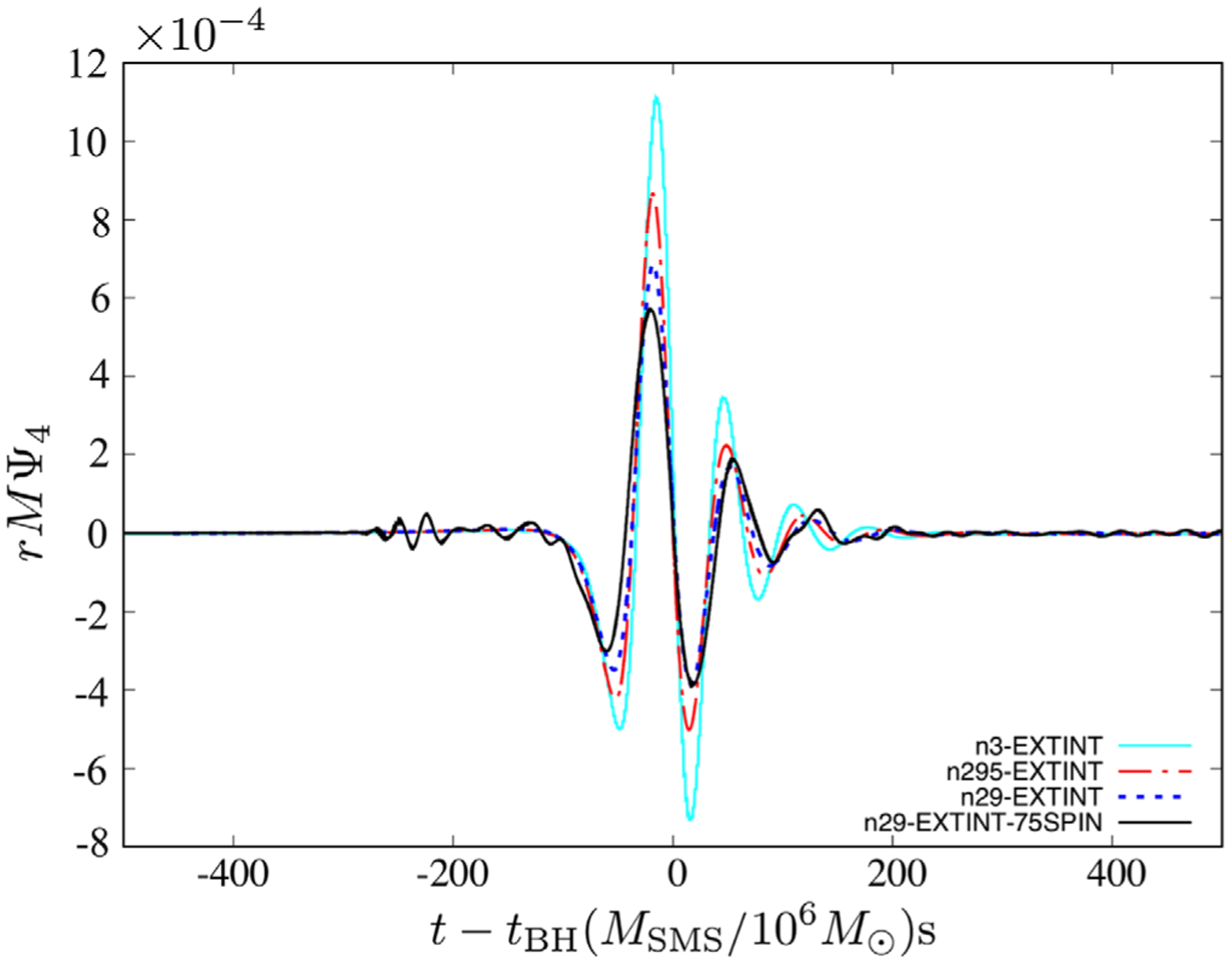
Real part of the (l, m) = (2, 0) mode of Ψ₄ as a function of t − t_BH for the cases with interior and exterior B-field at an extraction radius R_ext ~ 100M. The cyan curve represents the n3-EXTINT case displayed in [27]. Cases with other B-field configurations share similarity with their counterparts in the figure.

V. SUMMARY AND CONCLUSIONS

In this work, we extended our earlier calculations [27] of the magnetorotational collapse of SMSs in which radiation pressure alone is present(Γ = 4/3, or n = 3) Such a model applies to SMSs with M ≳ 10⁶M_⊙. Hence we have performed full GRMHD simulations of collapsing of SMSs with masses ≳10⁴ − 10⁵M_⊙ for which gas pressure represents a significant perturbation [12,94,102]. We considered stellar models described by a polytropic EOS with Γ ≳ 4/3, or equivalently n ≲ 3, which effectively incorporates a gas pressure perturbation. Such a model also crudely describes massive Pop III stars. We also studied the impact of the initial stellar rotation profile and the initial magnetic field configuration on the final outcome of the SMS remnant. To be consistent with our previous study [27], we set the initial magnetic-to-rotational-kinetic energy to 0.1.

We focus on uniformly rotating configurations spinning at mass-shedding and on the verge of collapse due to a relativistic radial instability. For uniformly rotating cases, the evolution process is similar to the n = 3 cases presented in [27] with the same initial magnetic field configuration. For smaller characteristic masses (smaller n), the stars collapse in a shorter period. The outcome in all cases is a spinning black hole surrounded by an accretion disk. For smaller initial n and thus smaller M, the BH has a greater M_BH/M and thus a smaller M_disk/M, and a smaller a_BH/M_BH. All the black hole parameters are consistent with various previous semianalytic and numerical studies in [18,24,26,38,63]. For SMSs with M ≳ 10⁶M_⊙, the ratios M_BH/M, a_BH/M_BH and M_disk/M are universal numbers independent of mass [25]: M_BH/M ≈ 0.9, a_BH/M_BH ≈ 0.75 and M_disk/M ≈ 0.1. Furthermore, for all magnetized cases, the final ${\dot{M}}_{\text{BH}}$ is roughly the same (~0.1 − 1M_⊙/s) as is the Poynting luminosity (L_EM ~ 10^52±1 erg/s), independent of M. These are consistent with the n = 3 cases and with the unified analytic model in [32].

For the cases with reduced spin Ω = 0.75Ω_shedd, we found that almost all the matter falls into the black hole, with only ~0.3% of the total mass remaining to form the disk. Correspondingly, L_EM is approximately one order of magnitude smaller than its uniformly rotating counterpart. On the contrary, the collapse of a differentially rotating star results in a massive disk with M_disk/M ~ 0.18 and the highest luminosity L_EM ~ 10^53.5 erg/s.

We find that all appreciably magnetized disks launch incipient jets. We confirm the likelihood that the BZ mechanism generates the Poynting luminosity in the jets. The gravitational waveforms for n ≲ 3 show strong resemblance to their n = 3 counterparts. It is thus expected that GW detectors like LISA and DECIGO are capable of observing the GW signals from such events [27]. The specific angular momentum profiles in the post-BH disk show that the disk is stable with respect to PPI even without the magnetic field, and such stability is probably strengthened in presence of the magnetic field. Additionally, the magnitude of the Poynting luminosity, which is insensitive to the stellar mass M, suggests that detecting the EM counterpart radiation from magnetized, massive, stellar collapses by GRB detectors like Fermi and Swift is quite feasible [108,109]. Therefore, the study of and search for SMSs or massive Pop III stars could provide a promising avenue for advancing multimessenger astronomy research.

An extensive survey of different rotation profiles is clearly needed to strengthen our conclusion [e.g., Eq. (14)] regarding the EM luminosity in the case of differentially rotating stars. However, the results reported here, along with the simulations of supermassive black holes surrounded by accretion disk in [110], the simulations of black hole-neutron star mergers in [34], and those of binary neutron star mergers [35] suggest that indeed there maybe a narrow range of expected EM luminosity in accord with Eq. (14) and the analysis in [32].

References

- [1].Bañados E, Venemans BP, Mazzucchelli C, Farina EP, Walter F, Wang F, Decarli R, Stern D, Fan X, Davies F et al. , Nature (London) 553, 473 (2018).29211709 [Google Scholar]
- [2].Mortlock DJ et al. , Nature (London) 474, 616 (2011). [DOI] [PubMed] [Google Scholar]
- [3].Wu X-B, Wang F, Fan X, Yi W, Zuo W, Bian F, Jiang L, McGreer ID, Wang R, Yang J et al. , Nature (London) 518, 512 (2015). [DOI] [PubMed] [Google Scholar]
- [4].Smith A, Bromm V, and Loeb A, Astron. Geophys 58, 3.22 (2017). [Google Scholar]
- [5].Rees MJ, Annu. Rev. Astron. Astrophys 22, 471 (1984). [Google Scholar]
- [6].Begelman MC, Volonteri M, and Rees MJ, Mon. Not. R. Astron. Soc 370, 289 (2006). [Google Scholar]
- [7].Begelman MC, Mon. Not. R. Astron. Soc 402, 673 (2010). [Google Scholar]
- [8].Madau P and Rees MJ, Astrophys. J 551, L24 (2001). [Google Scholar]
- [9].Volonteri M, Astron. Astrophys. Rev 18, 279 (2010). [Google Scholar]
- [10].Karlsson T, Bromm V, and Bland-Hawthorn J, Rev. Mod. Phys 85, 809 (2013). [Google Scholar]
- [11].Chen K-J, Heger A, Woosley S, Almgren A, Whalen DJ, and Johnson JL, Astrophys. J 790, 162 (2014). [Google Scholar]
- [12].Bond R, Arnett WD, and Carr BJ, Astrophys. J 280, 825 (1984). [Google Scholar]
- [13].Heger A and Woosley SE, Astrophys. J 567, 532 (2002). [Google Scholar]
- [14].Rakavy G, Shaviv G, and Zinamon Z, Astrophys. J 150, 131 (1967). [Google Scholar]
- [15].Woosley SE, in Saas-Fee Advanced Course 16: Nucleo-synthesis and Chemical Evolution, edited by Audouze J, Chiosi C, and Woosley SE (Geneva Observatory, Sauverny, Switzerland, 1986), p. 1. [Google Scholar]
- [16].Alvarez MA, Wise JH, and Abel T, Astrophys. J 701, L133 (2009). [Google Scholar]
- [17].Shapiro SL and Teukolsky SA, Astrophys. J 234, L177 (1979). [Google Scholar]
- [18].Baumgarte TW and Shapiro SL, Astrophys. J 526, 941 (1999). [DOI] [PubMed] [Google Scholar]
- [19].Saijo M, Baumgarte TW, Shapiro SL, and Shibata M, Astrophys. J 569, 349 (2002). [DOI] [PubMed] [Google Scholar]
- [20].Bañados E Venemans BP, Mazzucchelli C, Farina EP, Walter F, Wang F, Decarli R, Stern D, Fan X, Davies FB, Hennawi JF, Simcoe RA, Turner ML, Rix H-W, Yang J, Kelson DD, Rudie G, and Winters JM, Nature (London), 553, 473 (2018).29211709 [Google Scholar]
- [21].Wagoner RV, Annu. Rev. Astron. Astrophys 7, 553 (1969). [Google Scholar]
- [22].Zel’dovich YB and Novikov ID, Relativistic Astrophysics, Vol. I: Stars and Relativity (University of Chicago Press, Chicago, 1971). [Google Scholar]
- [23].Shapiro SL, Astrophys. J 544, 397 (2000). [Google Scholar]
- [24].Shibata M and Shapiro SL, Astrophys. J. Lett 572, L39 (2002). [Google Scholar]
- [25].Shapiro S and Shibata M, Astrophys. J 572, L39 (2002). [Google Scholar]
- [26].Liu YT, Shapiro SL, and Stephens BC, Phys. Rev. D 76, 084017 (2007). [Google Scholar]
- [27].Sun L, Paschalidis V, Ruiz M, and Shapiro S, Phys. Rev. D 96, 043006 (2017). [DOI] [PMC free article] [PubMed] [Google Scholar]
- [28].GRB 140304A data, http://swift.gsfc.nasa.gov/archive/grb_table/140304A/.
- [29].GRB 090423 data, http://swift.gsfc.nasa.gov/archive/grb_table/090423/.
- [30].Tornatore L, Ferrara A, and Schneider R, Mon. Not. R. Astron. Soc 382, 945 (2007). [Google Scholar]
- [31].Johnson JL, Vecchia CD, and Khochfar S, Mon. Not. R. Astron. Soc 428, 1857 (2013). [Google Scholar]
- [32].Shapiro SL, Phys. Rev. D 95, 101303 (2017). [DOI] [PMC free article] [PubMed] [Google Scholar]
- [33].Blandford R and Znajek R, Mon. Not. R. Astron. Soc 179, 433 (1977). [Google Scholar]
- [34].Paschalidis V, Ruiz M, and Shapiro M, Astrophys. J 806, L14 (2015). [Google Scholar]
- [35].Ruiz M, Lang R, Paschalidis V, and Shapiro S, Astrophys. J 824, L6 (2016). [DOI] [PMC free article] [PubMed] [Google Scholar]
- [36].Fuller GM, Woosley SE, and Weaver TA, Astrophys. J 307, 675 (1986). [Google Scholar]
- [37].Montero PJ, Janka H-T, and Müller E, Astrophys. J 749, 37 (2012). [Google Scholar]
- [38].Shapiro SL, Astrophys. J 610, 913 (2004). [Google Scholar]
- [39].Shibata M, Uchida H, and Sekiguchi Y, Astrophys. J 818, 157 (2016). [Google Scholar]
- [40].Shibata M, Sekiguchi Y, Uchida H, and Umeda H, Phys. Rev. D 94, 021501 (2016). [Google Scholar]
- [41].Butler SP, Lima AR, Baumgarte TW, and Shapiro SL, Mon. Not. R. Astron. Soc 477, 3694 (2018). [DOI] [PMC free article] [PubMed] [Google Scholar]
- [42].New KCB and Shapiro SL, Astrophys. J 548, 439 (2001). [Google Scholar]
- [43].Shapiro SL, AIP Conf. Proc 686, 50 (2003). [Google Scholar]
- [44].Bodenheimer P and Ostriker JP, Astrophys. J 180, 159 (1973). [Google Scholar]
- [45].Tassoul J-L, Theory of Rotating Stars (Princeton University Press, Princeton, NJ, 1978). [Google Scholar]
- [46].Saijo M, Astrophys. J 615, 866 (2004). [Google Scholar]
- [47].Zink B, Stergioulas N, Hawke I, Ott CD, Schnetter E, and Müller E, Phys. Rev. Lett 96, 161101 (2006). [DOI] [PubMed] [Google Scholar]
- [48].Reisswig C, Ott C, Abdikamalov E, Haas R, Moesta P, and Schnetter E, Phys. Rev. Lett 111, 151101 (2013). [DOI] [PubMed] [Google Scholar]
- [49].Armano M. e. a., Phys. Rev. Lett 116, 231101 (2016). [DOI] [PubMed] [Google Scholar]
- [50].Babak S, Hannam M, Husa S, and Schutz B, arXiv:0806.1591
- [51].Gendre B, Stratta G, Atteia JL, Basa S, Boër M, Coward DM, Cutini S, D’Elia V, Howell EJ, Klotz A et al. , Astrophys. J 766, 30 (2013). [Google Scholar]
- [52].Stratta G, Gendre B, Atteia JL, Bor M, Coward DM, Pasquale MD, Howell E, Klotz A, Oates S, and Piro L, Astrophys. J 779, 66 (2013). [Google Scholar]
- [53].Gehrels N and Razzaque S, Front. Phys 8, 661 (2013). [Google Scholar]
- [54].Papaloizou JCB and Pringle JE, Mon. Not. R. Astron. Soc 208, 721 (1984). [Google Scholar]
- [55].Kiuchi K, Shibata M, Montero PJ, and Font JA, Phys. Rev. Lett 106, 251102 (2011). [DOI] [PubMed] [Google Scholar]
- [56].Eddington AS, Mon. Not. R. Astron. Soc 79, 2 (1918). [Google Scholar]
- [57].Chandrasekhar S, An Introduction to the Study of Stellar Structure (The University of Chicago press, Chicago, Illinois, 1939). [Google Scholar]
- [58].Shapiro SL and Teukolsky SA, Black Holes, White Dwarfs, and Neutron Stars (John Wiley & Sons, New York, 1983). [Google Scholar]
- [59].Clayton DD, Principles of Stellar Evolution and Nucleo-synthesis (University of Chicago Press, Chicago, 1983). [Google Scholar]
- [60].Baumgarte TW and Shapiro SL, Astrophys. J 526, 937 (1999). [DOI] [PubMed] [Google Scholar]
- [61].Papaloizou JCB and Whelan JAJ, Mon. Not. R. Astron. Soc 164, 1 (1973). [Google Scholar]
- [62].Cook GB, Shapiro SL, and Teukolsky SA, Astrophys. J 398, 203 (1992). [Google Scholar]
- [63].Cook GB, Shapiro SL, and Teukolsky SA, Astrophys. J 422, 227 (1994). [Google Scholar]
- [64].Cook GB, Shapiro SL, and Teukolsky SA, Astrophys. J 424, 823 (1994). [Google Scholar]
- [65].Duez MD, Liu YT, Shapiro SL, and Stephens BC, Phys. Rev. D 69, 104030 (2004). [Google Scholar]
- [66].Zink B, Stergioulas N, Hawke I, Ott CD, Schnetter E, and Müller Phys E. Rev. D 76, 024019 (2007). [DOI] [PubMed] [Google Scholar]
- [67].Etienne ZB, Liu YT, and Shapiro SL, Phys. Rev. D 82, 084031 (2010). [Google Scholar]
- [68].Etienne ZB, Paschalidis V, Liu YT, and Shapiro SL, Phys. Rev. D 85, 024013 (2012). [Google Scholar]
- [69].Paschalidis V, Etienne ZB, and Shapiro SL, Phys. Rev. D 88, 021504 (2013). [Google Scholar]
- [70].Khan A, Paschalidis V, Ruiz M, and Shapiro SL, Phys Rev. D 97, 044036 (2018. [DOI] [PMC free article] [PubMed] [Google Scholar]
- [71].Shibata M and Nakamura T, Phys. Rev. D 52, 5428 (1995). [DOI] [PubMed] [Google Scholar]
- [72].Baumgarte TW and Shapiro SL, Phys. Rev. D 59, 024007 (1998). [Google Scholar]
- [73].Baker JG, Centrella J, Choi D-I, Koppitz M, and van Meter J, Phys. Rev. Lett 96, 111102 (2006). [DOI] [PubMed] [Google Scholar]
- [74].Campanelli M, Lousto CO, Marronetti P, and Zlochower Y, Phys. Rev. Lett 96, 111101 (2006). [DOI] [PubMed] [Google Scholar]
- [75].Hinder I, Buonanno A, Boyle M, Etienne ZB, Healy J et al. , Classical Quantum Gravity 31, 025012 (2014). [Google Scholar]
- [76].Ruiz M, Hilditch D, and Bernuzzi S, Phys. Rev. D 83, 024025 (2011). [Google Scholar]
- [77].Duez MD, Liu YT, Shapiro SL, and Stephens BC, Phys. Rev. D 72, 024028 (2005). [Google Scholar]
- [78].Farris BD, Gold R, Paschalidis V, Etienne ZB, and Shapiro S, Phys. Rev. Lett 109, 221102 (2012). [DOI] [PubMed] [Google Scholar]
- [79].Haiman Z, Astrophysics and Space Science Library 296, 293 (2012). [Google Scholar]
- [80].Regan JA, Johansson PH, and Wise JH, Astrophys. J 795, 137 (2014). [Google Scholar]
- [81].Rees MJ, Annu. Rev. Astron. Astrophys 22, 471 (1984). [Google Scholar]
- [82].Gnedin OY, Classical Quantum Gravity 18, 3983 (2001). [Google Scholar]
- [83].Shibata M, Uchida H, and Sekiguchi Y, Astrophys. J 818, 157 (2016). [Google Scholar]
- [84].Heger A, Fryer CL, and Woosley SE, Astrophys. J 567, 532 (2002). [Google Scholar]
- [85].Baraffe I, Heger A, and Woosley SE, Astrophys. J 550, 890 (2001). [Google Scholar]
- [86].Etienne ZB, Liu YT, Paschalidis V, and Shapiro SL, Phys. Rev. D 85, 064029 (2012). [Google Scholar]
- [87].Ruiz M and Shapiro SL, Phys. Rev. D 96, 084063 (2017). [DOI] [PMC free article] [PubMed] [Google Scholar]
- [88].Etienne ZB, Faber JA, Liu YT, Shapiro SL, Taniguchi K, and Baumgarte TW, Phys. Rev. D 77, 084002 (2008). [Google Scholar]
- [89].Ruiz M, Takahashi R, Alcubierre M, and Nunez D, Gen. Relativ. Gravit 40, 2467 (2008). [Google Scholar]
- [90].Etienne ZB, Liu YT, Shapiro SL, and Baumgarte TW, Phys. Rev. D 79, 044024 (2009). [Google Scholar]
- [91].Thornburg J, Classical Quantum Gravity 21, 743 (2004). [Google Scholar]
- [92].Dreyer O, Krishnan B, Shoemaker D, and Schnetter E, Phys. Rev. D 67, 024018 (2003). [Google Scholar]
- [93].Gold R, Paschalidis V, Etienne ZB, Shapiro SL, and Pfeiffer HP, Phys. Rev. D 89, 064060 (2014). [Google Scholar]
- [94].Uchida H, Shibata M, Yoshida T, Sekiguchi Y, and Umeda H, Phys. Rev. D 96, 083016 (2017). [Google Scholar]
- [95].Shapiro SL, arXiv:astro-ph/0304202.
- [96].Matsumoto T, Nakauchi D, Ioka K, Heger A, and Nakamura T, Astrophys. J 810, 64 (2015). [Google Scholar]
- [97].Matsumoto T, Nakauchi D, Ioka K, and Nakamura T, Astrophys. J 823, 83 (2016). [Google Scholar]
- [98].McKinney JC and Gammie CF, Astrophys. J 611, 977 (2004). [Google Scholar]
- [99].Ackermann M, Ajello M, Asano K, Axelsson M, Baldini L, Ballet J, Barbiellini G, Bastieri D, Bechtol K, Bellazzini R et al. , Astrophys. J. Suppl. Ser 209, 11 (2013). [Google Scholar]
- [100].Toma K, Yoon S-C, and Bromm V, Space Sci. Rev 202, 159 (2016). [Google Scholar]
- [101].Li Y, Zhang B, and Lü H-J, Astrophys. J. Suppl. Ser 227, 7 (2016). [Google Scholar]
- [102].Shibata M, Sekiguchi Y, Uchida H, and Umeda H, Phys. Rev. D 94, 021501 (2016). [Google Scholar]
- [103].eLISA, Note for eLISA cosmology working group on sensitivity curve and detection, eLISA Document Version 0.3.
- [104].Yagi K and Tanaka T, Prog. Theor. Phys 123, 1069 (2010). [Google Scholar]
- [105].Yagi K, Tanahashi N, and Tanaka T, Phys. Rev. D 83, 084036 (2011). [Google Scholar]
- [106].Bugli M, Guilet J, Müller E, Del Zanna L, Bucciantini N, and Montero PJ, Mon. Not. R. Astron. Soc 475, 108 (2018). [Google Scholar]
- [107].Papaloizou JCB and Pringle JE, Mon. Not. R. Astron. Soc 213, 799 (1985). [Google Scholar]
- [108].Bosnjak Z, Got D, Bouchet L, Schanne S, and Cordier B, Astron. Astrophys 561 (2014). [Google Scholar]
- [109].Connaughton V, Pelassa V, Briggs M, Jenke P, Troja E, McEnery J, and Blackburn L, EAS Publ. 61, 657 (2013). [Google Scholar]
- [110].Khan A, Paschalidis V, Ruiz M, and Shapiro SL, Phys. Rev. D 97, 044036 (2018). [DOI] [PMC free article] [PubMed] [Google Scholar]