Improving deconvolution methods in biology through open innovation competitions: an application to the connectivity map

Abstract

Motivation

Do machine learning methods improve standard deconvolution techniques for gene expression data? This article uses a unique new dataset combined with an open innovation competition to evaluate a wide range of approaches developed by 294 competitors from 20 countries. The competition’s objective was to address a deconvolution problem critical to analyzing genetic perturbations from the Connectivity Map. The issue consists of separating gene expression of individual genes from raw measurements obtained from gene pairs. We evaluated the outcomes using ground-truth data (direct measurements for single genes) obtained from the same samples.

Results

We find that the top-ranked algorithm, based on random forest regression, beat the other methods in accuracy and reproducibility; more traditional gaussian-mixture methods performed well and tended to be faster, and the best deep learning approach yielded outcomes slightly inferior to the above methods. We anticipate researchers in the field will find the dataset and algorithms developed in this study to be a powerful research tool for benchmarking their deconvolution methods and a resource useful for multiple applications.

Availability and implementation

The data is freely available at clue.io/data (section Contests) and the software is on GitHub at https://github.com/cmap/gene_deconvolution_challenge

Supplementary information

Supplementary data are available at Bioinformatics online.

1 Introduction

A recurring problem in biomedical research is how to isolate distinct populations (cell types, tissues and genes) from composite measures obtained by a single analyte or sensor. This deconvolution problem often stems from the prohibitive cost of profiling each population separately (Cleary et al., 2017; Subramanian et al., 2017) and has important implications for the analysis of transcriptional data in mixed samples (Newman et al., 2015; Shen-Orr et al., 2010; Zaitsev et al., 2019; Zhong and Liu, 2011), single-cell data (Deng et al., 2019), the study of cell dynamics (Lu et al., 2003) and imaging data (Preibisch et al., 2014).

In the context of gene expression analysis, available deconvolution algorithms offer several advantages but have limitations as well (Shen-Orr et al., 2010; Shen-Orr and Gaujoux, 2013). Advanced machine learning techniques can help overcome some of the shortcomings. However, these approaches can be hard to benchmark because of the scarcity of ground truth data (methods are often trained and have their results validated on synthetic data) and difficulties in achieving proper model selection and parameter optimization that often require substantial expertise, which may not be available in every lab.

Motivated by examples of successful challenges for the development of machine learning solutions (Blasco et al., 2019; Good and Su, 2013; Lakhani et al., 2013), we report the results of an open competition, called the D-Peak Challenge, that we designed to address a gene-expression deconvolution problem for the NIH Library of Integrated Network-based Cellular Signatures (LINCS), also known as the Connectivity Map (CMap).

CMap is a catalog of over a million human gene-expression profiles (Subramanian et al., 2017) generated using a bead-based assay called L1000. This assay focuses on a reduced transcriptome consisting of approximately 1000 human genes, called landmarks. One critical issue is that the assay screening capacity is limited to a maximum of 500 available bead colors per screen, which is less than the desired 1000 landmarks. To address this problem, the CMap team has developed a procedure that couples each unique bead color with two genes and then relies on a deconvolution algorithm, called d-peak, to separate the expression of the 1000 landmark genes from the 500 bead measurements.

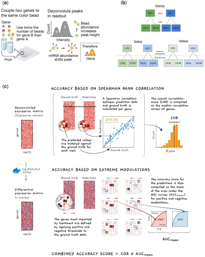
Figure 1a provides a schematic representation of the deconvolution procedure. All the landmark genes are grouped into pairs of two. Each pair is tagged with a unique bead color in separate batches and mixed in a 2:1 proportion before use. Luminex scanners examine the mixture and return two values from each bead: the color, identifying the pair and the signal intensity, reflecting the combined mRNA expression of the two genes per bead. This step yields an intensity distribution of the beads that generally consists of two peaks (see Fig. 1a), a larger one that designates the gene expression in high proportion and a smaller one representing the other gene. At this point, a k-means clustering algorithm partitions the distribution into k clusters by minimizing the within-cluster sum of squares. It then associates the largest (smallest) cluster to the gene with a higher (lower) bead proportion, assigning the cluster’s median value to the corresponding gene.

Fig. 1.

(a) Schematic of the deconvolution procedure, (b) overview of the data generated for the contest grouped into three pairs with six plates each: two perturbation types (compounds and shRNA) times three detection plates (two for UNI and 1 for DUO), and (c) illustration of the scoring methods for the evaluation of submissions

Young et al. (2016) points out some of the limitations of the current k-means algorithm. Prominently, when scanners detect outliers with very low intensity, the algorithm can form artificial clusters that may harm downstream analysis. This technical problem has attracted considerable attention and several solutions have been proposed: Young et al. (2016) proposes a Gaussian model-based clustering approach; Li et al. (2017) combines a Gaussian mixture model with an outlier detection method; and Qiu et al. (2020) suggests a Bayesian-based procedure. However, there remain significant opportunities for further innovation.

This study adds to existing work by providing a novel dataset (available online on CMap’s portal at clue.io/data) that can be used as ground truth for training/evaluating new deconvolution techniques. It also reports the best machine learning methods devised by the competitors who have won the D-peak challenge (source codes available on GitHub at github.com/cmap/gene\_deconvolution\_challenge). These methods outperformed the L1000 benchmark in pre-specified metrics of accuracy and computational speed that were computed using examples unseen by the competitors.

2 Materials and methods

Figure 1b shows a schematic representation of the data generated for the challenge. The data consists of eighteen 384-well plates, each containing sets of compound and short hairpin RNA (shRNA) treatments for a total of 122 different perturbations (see Supplementary Material for a complete list) and with multiple replicates (4 and 10 for the shRNA and compound treatments, respectively). Multiple cell lines and perturbations were used to avoid any potential over-fitting. The compound and shRNA plates were arbitrarily grouped into pairs, and to avoid any potential information leakage each pair was profiled in a different cell line. The resulting lysates were amplified by Ligation Mediated Amplification (Subramanian et al., 2017).

The ground truth data was generated by splitting the product of amplification in two types of detection modes. The standard dual procedure (DUO), using two genes per bead color, and a more accurate procedure (UNI), using one gene per bead color. This yielded three pairs of data of six plates each (2 perturbation types × 3 detection plates: 2 for UNI and 1 for DUO) generated under comparable circumstances (Fig. 1b).

These data pairs were split into training, testing and hold out. The training data was available for all the contestants to develop and validate their solutions offline. The testing data was used for submission evaluation during the contest and to populate a live leaderboard. The holdout data was used for final evaluation and it was unseen to competitors to guard against over-fitting. Prizes were awarded based on performance on the holdout dataset.

Figure 1c shows a schematic representation of the scoring function that was used to evaluate submissions on their accuracy and computational speed (see Supplementary Material for the details).

Accuracy was assessed using two different metrics. One was the average gene-wise Spearman’s rank correlation between the deconvoluted expression values and the ground truth. The other was the Area Under the receiver operating characteristic Curve (AUC) in the prediction of extremely modulated genes (genes notably up- or down-regulated by perturbation in the UNI data).

Speed was assessed by executing each submission on comparable multi-core machines, thus allowing competitors to employ multithreading techniques, and the corresponding score was the average runtime in units of the benchmark runtime.

The challenge was hosted on Topcoder (Wipro, India), a popular crowdsourcing platform, and lasted for 21 days. A prize purse of $23 000 in cash was offered to competitors as an incentive to be divided among the top 9 submissions.

3 Results

The contest attracted 294 participants who made 820 submissions using a variety of different methods. Table 1 shows the classes of algorithms and performance for the top nine solutions, as ranked in the final leaderboard.

Table 1.

Overview of outcomes for the top nine competitors

Rank	Method	Language	Spearman correlation (%)	AUC extreme modulations (%)	Recovered gene knockdowns (%)	MSE	Mean inter-replicate correlation (%)	Time per plate (s)
1	Random forest regressor	Java	66.5	91.5	77.2	1	45.2	14.5
2	Gaussian mixture model	C++	65.4	91.4	75.7	1.1	43.1	4
3	Modified k-means	C++	64.6	91.2	77.8	2.2	41.9	10.5
4	ConvNet	Python/C++	64.8	91	76.6	2.4	41.8	25
5	Gaussian mixture model	Python/C++	64.6	90.9	75.7	1.3	41.9	36
6	Modified k-means	Python/C++	64.3	90.2	70.8	1.1	40.6	11.5
7	Boosted tree regressor	Python	64.5	91.1	77.2	1.7	41.9	50.5
8	Modified k-means	Python	65.1	90	69	1.2	43.7	35.5
9	Other	Java	63.9	89.9	75.1	1.5	39.6	4.5
BM	k-means	Matlab	63.2	89.2	73.9	3	38.9	247

Note: All the values are based on the holdout dataset; see the main text for the meaning. The maximum and minimum values in each column are in bold.

3.1 Top four algorithms

We begin the analysis of the results with a description of the algorithms used by the top four solutions.

The winning entry (submitted by a competitor from the United States with a degree in Physics from the University of Kansas) uses a random forest algorithm that combines predictions from ten different trees trained on sixty features derived from the data. These features consist of a combination of low-peak and high-peak estimates for each gene pair and aggregate measures to capture any systematic bias at the perturbation, analyte and plate level.

The second-placed entry (submitted by a competitor from Poland with a Master in Computer Science from the Lodz University of Technology) uses the Expectation-Maximization algorithm to fit the data to a mixture of two log-normal models for each gene pair where, instead of assuming a priori probability (the 2:1 ratio) of assignment to clusters, the algorithm tries to learn the actual ratio from the data by fitting a plate-wide distribution of cluster sizes.

The third-placed entry (submitted by a competitor from India with a Bachelor in Computer Science) modifies the standard k-means algorithm with a random initialization procedure that avoids local minima and is more robust to extreme outliers.

The fourth-placed entry (submitted by a competitor from Ukraine with a Bachelor in Computer Science from the Cherkasy National University) uses a Convolutional Neural Network (CNN). This algorithm first filters and transforms the data into a 32-bin histogram for each pair of genes. It uses the U-net architecture (Ronneberger et al., 2015) to provide an adequate representation of the data. It then assigns each of the bins to one of the two genes for each pair and predicts the median value. This final step uses two subnetworks with the same architecture. The model is trained using a mean squared error (MSE) loss function.

3.2 Deconvolution accuracy (Spearman correlation)

To assess improvements over the benchmark, we computed the deconvolution accuracy for each solution from the hold out set. Deconvolution accuracy was defined as the gene-wise Spearman rank correlation between the deconvolution data (obtained by applying each solution to the data generated using two genes per bead color) and the ground truth (generated using one gene per bead color).

All competitors showed significant improvement over the benchmark, with most competitors achieving a mean difference of about three percentage points (Table 1).

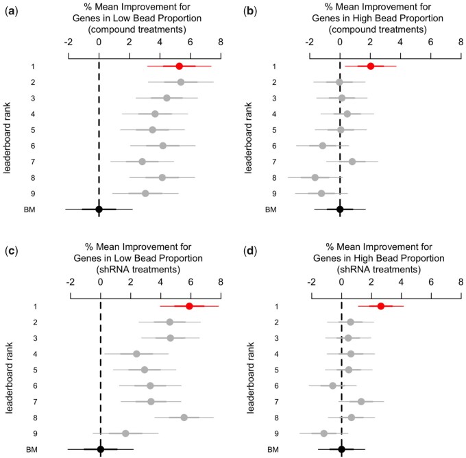
We expected performance to vary between genes in high and low bead proportion, given the differential number of beads for each gene. After disaggregation, we found that most improvements were limited to the subset of genes in low bead proportion, with nearly all competitors achieving gains in deconvolution accuracy ranging between four and six percentage points (Fig. 2a and c). For genes in high bead proportion, by contrast, only the winner was able to achieve a significant boost ranging between one and four percentage points (Fig. 2b and d). This pattern looked the same for both compound and shRNA samples (Fig. 2).

Fig. 2.

% mean difference (and 95% CI) in deconvolution accuracy between the benchmark (BM) and the competitors. Deconvolution accuracy is the gene-wise Spearman correlation between the ground truth and the deconvolution data (from the hold-out set). Most competitors achieved improvements over the benchmark for genes in low bead proportion (a, c) but performed about the same for genes in high bead proportion (b, d). The same pattern apply to shRNA (c, d) and compound samples as well (a, b)

To evaluate the extent to which the winning algorithm outperformed the others, we ranked the top-nine algorithms by the mean correlation metric for each gene (1 = highest, 9 = lowest). We then computed the percentage of genes for which a given algorithm was ranked first. The winner entry was ranked first for 30% of the genes, followed at some distance by the second-placed gaussian-mixture method (20%), and by the CNN method (13%). Thus, the top two submissions combined outperformed the rest for about half of the genes. Even so, all but a few algorithms were the best performers for at least 5% of the genes, suggesting some complementarity between these algorithms.

3.3 Detection of extreme modulation of gene expression

To assess improvements in detecting differential expression, we first examined the MSE between the differential values after deconvolution and the ground truth. Most competitors outperformed the benchmark on this metric (Table 1), with the top two solutions achieving a MSE of 1.0, representing a 70% reduction relative to the benchmark’s. However, this metric reflects average prediction errors that may not necessarily yield a higher detection accuracy of extreme modulation of gene expression (genes notably up or down regulated).

A more direct measure of detection accuracy was the AUC for the expected extreme modulation of genes in the ground truth and the corresponding predicted differential expressions obtained by deconvolution. The expected extreme modulations were defined as genes with an absolute differential expression generated in UNI (one gene per bead color) greater than a given cutoff.

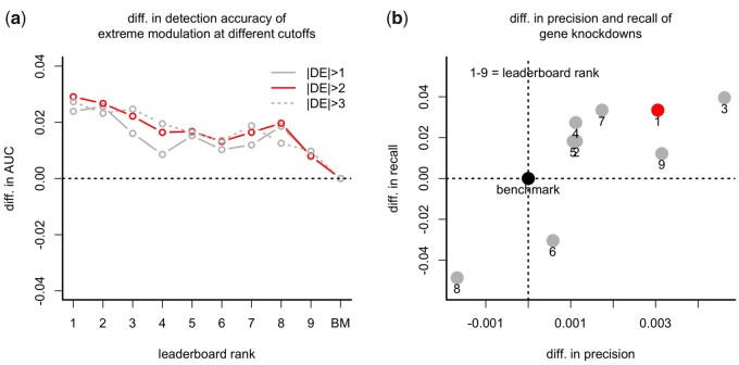
Nearly all competitors achieved significant improvements in this metric (Fig. 3a), with minor differences across different cutoffs (cutoff = 1, 2, 3). The largest gain was achieved by the winner with an AUC of nearly 3 percentage points greater than the benchmark.

Fig. 3.

(a) Difference in detection accuracy between the benchmark (BM) and the competitors. Detection accuracy is the AUC for the extreme modulation of genes in the ground-truth data and the corresponding predicted differential expressions obtained by deconvolution. Extreme modulations come from the differential expression of the UNI method at three different cutoffs (cutoff = 1, 2, 3). (b) difference in precision and recall of the targeted KD genes (shRNA samples) for the benchmark and the competitors

To illustrate the potential relevance of these improvements for downstream analysis, we computed the number of positives and true positives for the winning solution and the benchmark with a cutoff of two (see Supplementary Material for a descriptive table). The winner detected about 8000 less extreme modulations than the benchmark (63 828 and 72 161, respectively), thus being more conservative. However, after restricting the comparison to extreme modulations detected by UNI as well, the winning solution detects about 1891 more extreme modulations than the benchmark (37 002 and 35 111, respectively), representing a sensible increase in true positives.

We complemented the above analysis by using targeted gene knockdown (KD) experiments as the ground truth for a subset of data (Fig. 3b). These are experiments in which a landmark gene was targeted by an shRNA, and hence we expect to observe a significant decrease in expression for the targeted gene. We assessed the KD detection accuracy of each solution by computing the corresponding percentage of successful KD genes identified or recalled by the algorithm (defining a successful KD as one gene in which the DE value and the corresponding gene-wise rank in the experiment are less than a given threshold, −2 and 10 respectively). We computed the percentage recall for the UNI data as well, which yielded an estimate of the maximum achievable recall of 0.80. Relative to this level, nearly all algorithms achieved a good recall and precision, with values that were higher than the benchmark solution for all but two methods (Fig. 3b).

3.4 Reproducibility of gene expression changes

To assess the reproducibility of the results, we leveraged the several replicates per perturbation that are included in our dataset. Each shRNA and compound treatment has 4 and 10 replicates respectively.

To assess the inter-replicate variability of the results, we first computed the Median Absolute Deviation (MAD) of the differential expression for each gene across replicates. We then took the 75 h percentile for each of the 122 perturbations in our data. This yields 122 MAD observations per solution. We finally estimated the difference with the benchmark using a linear regression with fixed effects for the perturbation to control for differences in the level of reproducibility of each treatment (that were observed in the data).

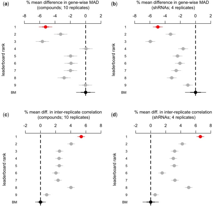
The top three solutions achieved significant reductions in variability compared to the benchmark (Fig. 4a and b), with the winner achieving a significant reduction between two and eight percentage points on the differential expression scale.

Fig. 4.

(a, b) % mean difference (and 95% CI) in gene-wise MAD between the benchmark (BM) and the competitors. The gene-wise MAD was computed across the 10 and 4 replicate differential expression values from the compound and shRNA samples, respectively. Differences were estimated using linear regression with fixed effects for each perturbation. (c, d) % mean difference (and 95% CI) in inter-replicate correlation between the benchmark and the competitors. The inter-replicate correlation is the 75th percentile pairwise Spearman Correlation Coefficient of the 10 and 4 replicate differential-expression signatures from the compound and shRNA samples, respectively. Differences were estimated using linear regression with fixed effects for each perturbation

To better understand the magnitude of these effects, we computed the pairwise inter-replicate Spearman correlation coefficient across all the differential expression signatures, a common measure of the reproducibility of L1000 signatures. We then took the 75 h percentile of the replicate correlation coefficients for each perturbation for a total of 122 correlation coefficients per method.

The winner shows a significant improvement over the benchmark in both samples (Fig. 4c and d), with an estimated gain in inter-replicate correlation that goes between 4 and 6 percentage points. This evidence suggests that the competitors’ solutions may help reduce the number of replicates that analysts may want to perform for a desired level of reproducibility.

3.5 Computational speed

The speed improvements over the benchmark were substantial (Table 1). While dpeak took about 4–5 min per plate, the fastest algorithm took as little as 4 s per plate (more than a 60× speedup compared to the benchmark) and the slowest was well below 1 min. These speed improvements are not directly attributable to the use of multiple cores, since both the benchmark and contestant algorithms leverage multi-core techniques. We observed no particular trade-off between speed and accuracy.

3.6 Ensembles of solutions

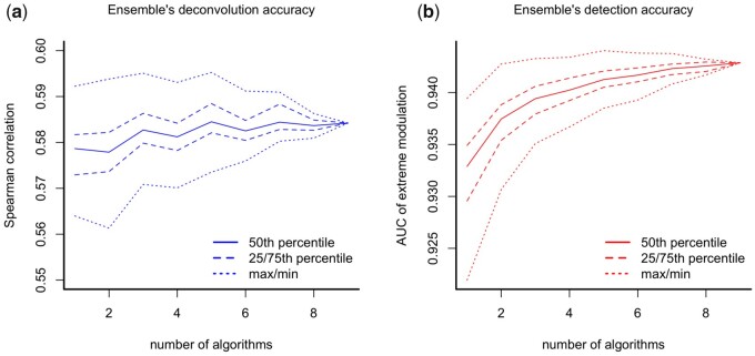
Lastly, we assessed the performance of ensembles combining the predictions of different computational methods by taking the median value across all 10 predictions (including the benchmark). By focusing on the subset of the data with shRNA experiments (ignoring the data with compound experiments), the performance in both Spearman correlation and the AUC metrics of the ensemble tended to increase with the number of models involved (Fig. 5). However, the maximum performance in both metrics tended to plateau (or even decrease) after combining the results of three or more models. This result suggested limited gains from having ensembles, although it may be worth exploring more sophisticated aggregation approaches.

Fig. 5.

(a) Performance in deconvolution accuracy (Spearman) and (b) detection accuracy (AUC) of an ensemble based on the median prediction of all possible combinations of a given size of the top nine algorithms plus the benchmark. The median performance of the ensemble tends to increase with its size. However, the maximum performance in both metrics tends to plateau (or even decrease) after the ensemble reaches a size equal to three

4 Discussion

Given the growing use of CMap for applied research, significant improvements in the methods used to analyze the L1000 data may have a remarkable impact on researchers in the field. Here, we have focused on one critical step in the pipeline that transforms raw data into data ready for analysis. That is the deconvolution of the expression of gene pairs measured by a single analyte. The key challenge was to isolate distinct genes from composite measurements trying to avoid artificial clusters generated by the assay, which is a recurrent problem in the analysis of gene expression.

Previous research has shown some limitations of the current default algorithm and has advanced possible solutions (Li et al., 2017; Qiu et al., 2020; Young et al., 2016). Existing solutions are extensions of classical model-based clustering used extensively to analyze genetic data (see Young et al., 2016) but do not include more recent machine learning methods, such as random forest clustering or neural networks.

We have shown how using a crowdsourcing competition leads to develop new algorithms for the deconvolution of L1000 data. We have assessed how these solutions performed using a novel dataset of transcriptional profiles for over 120 shRNA and compound experiments with several replicates for a total of 2200 gene expression of genes measured independently (UNI) and in tandem (DUO). This dataset constitutes now a public resource to all the researchers in this area interested in testing their deconvolution approaches.

Competitors’ solutions compared favorably against the current d-peak solution. The best method was a random forest, a collection of decision tree regressors, with feature engineering to capture possible systematic bias at the perturbation, analyte and plate level. This method achieved (i) the highest correlation between the ground-truth and the corresponding deconvolution data, (ii) the lowest inter-replicate variation of differential expression values and (iii) compared to the benchmark, was able to detect more than a thousand additional extreme modulation of genes while reducing the false positives at the same time. We have further shown that most of the gains were for genes in low bead proportion versus genes in high bead proportion, where the algorithm was good at mitigating the discrepancy in variability between the genes measured with different bead numbers.

We have also shown that the random-forest approach achieves these gains with only ten trees on sixty features. Therefore the algorithm is also relatively fast and easy to implement. By comparison, the fastest one used a more traditional Gaussian mixture model (with plate-level adjustments) but was less accurate.

While our analysis provides evidence of the tremendous potential of using random forests for deconvolution of gene expression data, it remains unclear to what extent the performance boost will apply more generally to other analyses of genetic data. Yet, another caveat to the generalizability of our results lies in the method for selecting the winners. By applying all entries to the hold-out dataset and reporting the results of the best-performing ones, we may have over-estimated the accuracy of the winning methods. However, we have shown improvements consistent in various metrics and across several approaches. This consistency leads us to believe that researchers will value the competitors’ solutions and use them as a practical resource to improve the quality of the analysis of L1000 data.

Funding

This work was funded by the Eric and Wendy Schmidt Foundation, NASA Center of Collaborative Excellence, and the Kraft Precision Medicine Accelerator & Division of Research and Faculty Development at the Harvard Business School. The CMap competitions were supported in part by the National Institutes of Health Common Funds Library of Integrated Network-based Cellular Signatures (LINCS) program [U54HG006093] and National Institutes of Health Big Data to Knowledge (BD2K) program [5U01HG008699].

Conflict of Interest: none declared.

References

- Blasco A. et al. (2019) Advancing computational biology and bioinformatics research through open innovation competitions. PLoS One, 14, e0222165–17. [DOI] [PMC free article] [PubMed] [Google Scholar]
- Cleary B. et al. (2017) Efficient generation of transcriptomic profiles by random composite measurements. Cell, 171, 1424–1436. [DOI] [PMC free article] [PubMed] [Google Scholar]
- Deng Y. et al. (2019) Scalable analysis of cell-type composition from single-cell transcriptomics using deep recurrent learning. Nat. Methods, 16, 311–314. [DOI] [PMC free article] [PubMed] [Google Scholar]
- Good B.M., Su A.I. (2013) Crowdsourcing for bioinformatics. Bioinformatics, 29, 1925–1933. [DOI] [PMC free article] [PubMed] [Google Scholar]
- Lakhani K.R. et al. (2013) Prize-based contests can provide solutions to computational biology problems. Nat. Biotechnol., 31, 108–111. [DOI] [PMC free article] [PubMed] [Google Scholar]
- Li D. et al. (2017) l1kdeconv: an r package for peak calling analysis with LINCS L1000 data. BMC Bioinformatics, 18, 1–7. [DOI] [PMC free article] [PubMed] [Google Scholar]
- Lu P. et al. (2003) Expression deconvolution: a reinterpretation of DNA microarray data reveals dynamic changes in cell populations. Proc. Natl. Acad. Sci. USA, 100, 10370–10375. [DOI] [PMC free article] [PubMed] [Google Scholar]
- Newman A.M. et al. (2015) Robust enumeration of cell subsets from tissue expression profiles. Nat. Methods, 12, 453–457. [DOI] [PMC free article] [PubMed] [Google Scholar]
- Preibisch S. et al. (2014) Efficient Bayesian-based multiview deconvolution. Nat. Methods, 11, 645–648. [DOI] [PMC free article] [PubMed] [Google Scholar]
- Qiu Y. et al. (2020) A Bayesian approach to accurate and robust signature detection on LINCS L1000 data. Bioinformatics, 36, 2787–2795. [DOI] [PMC free article] [PubMed] [Google Scholar]
- Ronneberger O. et al. (2015) U-net: convolutional networks for biomedical image segmentation. In: International Conference on Medical Image Computing and Computer-Assisted Intervention. Springer, Cham, Switzerland, pp. 234–241.
- Shen-Orr S.S., Gaujoux R. (2013) Computational deconvolution: extracting cell type-specific information from heterogeneous samples. Curr. Opin. Immunol., 25, 571–578. [DOI] [PMC free article] [PubMed] [Google Scholar]
- Shen-Orr S.S. et al. (2010) Cell type-specific gene expression differences in complex tissues. Nat. Methods, 7, 287–289. [DOI] [PMC free article] [PubMed] [Google Scholar]
- Subramanian A. et al. (2017) A next generation connectivity map: L1000 platform and the first 1,000,000 profiles. Cell, 171, 1437–1452. [DOI] [PMC free article] [PubMed] [Google Scholar]
- Young W.C. et al. (2016) Model-based clustering with data correction for removing artifacts in gene expression data. Ann. Appl. Stat., 11, 1998–2026. [DOI] [PMC free article] [PubMed] [Google Scholar]
- Zaitsev K. et al. (2019) Complete deconvolution of cellular mixtures based on linearity of transcriptional signatures. Nat. Commun., 10, 2209. [DOI] [PMC free article] [PubMed] [Google Scholar]
- Zhong Y., Liu Z. (2011) Gene expression deconvolution in linear space. Nat. Methods, 9, 8–9. [DOI] [PubMed] [Google Scholar]
Associated Data
This section collects any data citations, data availability statements, or supplementary materials included in this article.