

Abstract

Comprehensive thermochemical treatment (pyrolysis and combustion) is considered to be an efficient method for treatment of oil sludge (OS) or utilization as a heat source. However, combustion of oil sludge char (OSC), the byproduct from OS pyrolysis, is difficult and energy-consuming due to the high ash content and low heating value. In this study, co-combustion of OSC with biomass is proposed, aiming at the efficient thermal treatment with heat recovery. The thermal characteristics, kinetics, and interactive mechanisms of co-combustion of OSC with raw wood (RW) or hydrothermally treated wood (HW) employing thermogravimetric analysis were investigated. The obtained results indicated that RW blending with OSC resulted in negative interactions with decreasing the apparent activation energies (E) of RW, attributed to the inhibited diffusion of volatiles. The developed porous structure in HW effectively promoted volatile matter diffusion. Coupled with the catalytic support by metal oxides in OSC, HW blending yielded positive interactions during co-combustion despite the increased E. The results showed that diffusion models were the most efficient mechanism for OSC/RW combustion. However, chemical reactions were found to be the rate-determining steps for OSC/HW combustion. The catalytic effect of inorganic elements and their physical influence on heat and mass transfer can control the co-combustion performance of OSC and biomass. The findings could offer reference information for understanding OSC co-combustion and provide a basis for implementing and optimizing the co-combustion between biomass and ash-rich waste.
1. Introduction
Oil sludge (OS) is an undesired but inevitable hazardous byproduct of the petroleum industry. It is estimated that every 500 tons of crude oil will produce 1 ton of OS and the global volume of accumulated OS has reached 1 billion, where China is one of the largest producers, with annual production over 3 million tons.1,2 Recently, OS has been classified by many countries due to its inherent high petroleum and/or heavy metal contents, which pose a severe threat to human health and the eco-environment without proper disposal.2 Considering these petroleum hydrocarbons, direct landfill or discharge is not advisable, which conversely makes thermochemical treatment (incineration/combustion, pyrolysis, and gasification) one of the most attractive and high-potential methods for OS disposal. Therefore, a comprehensive thermochemical treatment (CTT), combining pyrolysis and combustion, has been regarded as an efficient and clean method for OS disposal and utilization.3,4 In this process, OS pyrolysis is first conducted to recover light oil and combustible gas. The derived oil sludge char (OSC) subsequently goes to combustion treatment for final disposal and heat recovery.5 This integrated approach has also been widely applied to effectively dispose and utilize oil sand, oil shale, and coal.6,7 EU countries also recommend combustion/incineration for waste treatment for its harmless nature and effective final disposal.8 However, OSC itself poses a low calorific value, and a large amount of additional energy is consumed for combustion treatment. In addition, high ash content of OSC might cause troubles such as slag fouling in combustion processes. They finally reduce the economic benefit of the CTT approach. Because CTT itself is an energy-intensive process, it requires necessary measures to reduce the high energy consumption and operational cost. Previous studies pointed out that recycling OS ash as a catalyst for OS pyrolysis and incorporating steam injection could potentially allow the CTT to be a self-sufficient system, as well as realizing efficient energy recovery.3 To address this limitation, co-combustion might also be cost-effective and promising, in which OSC can be efficiently treated. On the other hand, from a commercial point of view, the relevant companies engaged in combustion can obtain additional income, which is a win–win measure. Considering the rapid depletion of fossil fuels and the emission reduction requirement of greenhouse gas, renewable green energy resources could be candidate fuels for co-combustion.9
Biomass, one of the leading renewable energy resources, has attracted worldwide attention.10 Through proper utilization, biomass can act as an alternative fuel and play a supplementary role in meeting the world’s energy demand. Among biomass utilization methods, combustion is the most efficient and sustainable technology due to its high reactivity and carbon-neutral characteristic.11 Many researchers have conducted systematic techno-economic analyses on the co-combustion of coal and biomass.12−14 These results confirmed the vast potential of biomass in replacing fossil fuel as an energy source. Given these aspects, co-combustion of biomass and other solid waste is a promising measurement for waste treatment, especially for the wastes with high ash content, and cannot be directly landfilled, during which these wastes could be effectively disposed off and the additional value of biomass could be recovered. Previous studies pointed out that biomass blending could effectively improve the combustion properties of OSC. Gong et al.15 and Wang et al.16 studied co-combustion of OSC with microalgae residues. Their results demonstrated that microalgae residue addition promoted the combustion of volatile matters and reduced heavy metal ecotoxicity in combustion fly ash. Moreover, SO2 emission from the co-combustion was reduced due to the catalytic cracking effect of metal and metal oxides in OSC. However, there could be some operational problems because of the alkali and alkaline earth metals (AAEMs) in biomass fuel.17 The AAEMs in biomass are prone to cause fouling and slagging problems, which would impede the heat transfer, reduce the combustion reactivity, shorten the usage of the combustor, and thereby limit the large-scale application of (co-)combustion.18,19
Pretreatment of biomass prior to (co-)combustion could be an effective solution to the abovementioned problems and improving its combustion characteristics. Hydrothermal treatment (HTT), which is defined as a treatment of biomass in hot compressed water at temperatures within 180–260 °C (also referred to hydrothermal carbonization in this temperature range), has been regarded as a promising and environmentally acceptable method to upgrade biomass such as forest residues, agriculture waste, and sewage sludge.20 The hydrochars, generated by HTT, exhibit ameliorated homogeneity and higher fuel properties compared to raw biomass, such as lower oxygen content, higher carbon content, higher calorific values, and enhanced reactivity.21 On the other hand, most of the AAEMs are removed during HTT and the derived problems (fouling and slagging) can be avoided or greatly mitigated. In recent years, extensive studies on the co-combustion of HTT-modified biomass with solid waste by thermogravimetric analysis (TGA) have been reported. For example, Parshetti et al.22 performed co-combustion of empty fruit bunch (EFB), coal, and their respective hydrothermally treated hydrochars (HT-EFB and HT-coal). Their results indicated that the blend of HT-EFB (50%) and HT-coal (50%) showed the best combustion performance, with a twice higher corresponding combustion characteristic factor value than raw individual samples and their blends. What is more, the co-combustion of hydrochars reduced emissions of toxic (CO) and greenhouse (CH4 and CO2) gases. Yao et al.23 pointed out that the combustion characteristics of oil shale could be improved by mixing HTT hydrochar. The interactions between two feedstocks accelerated their decomposition rate at low temperatures and reduced the activation energy at a certain blending ratio.
However, to the best of the author’s knowledge, current research on co-combustion of OSC and biomass is limited to raw biomass utilization to improve the combustion characteristics of OSC. The interactive mechanisms of OSC/biomass co-combustion, such as the nature of synergy/inhibition that occurs during co-combustion of OSC/biomass, are still uncertain. Furthermore, the AAEMs in biomass could also act as catalysts during co-combustion in addition to causing fouling and slagging problems.24 Therefore, the removal of AAEMs after HTT might help identify the interactive mechanisms of OSC co-combustion with biomass when compared with OSC solo combustion and raw OSC/biomass co-combustion. On the other hand, kinetic analysis of OSC/biomass co-combustion is a prerequisite to understand reaction-based mechanisms and scale it up for industrial applications, which still needs more in-depth investigation.
TGA is one of the most used techniques to rapidly investigate and provide a quantitative method for detailed observation on thermal events and kinetics during the combustion of solid fuel, such as coal and biomass.25,26 The information obtained from TGA combustion profiles could be used to predict the industrial-scale combustion. Although TGA cannot be directly extrapolated to other equipment at a larger scale, it is very useful to offer fundamental referential opinions for the implementation and optimization of the co-combustion field.27 In this study, the TGA analysis was used to analyze the combustion behaviors of OSC, biomass, hydrochar, and their respective blends (OSC/biomass and OSC/hydrochar). The interactions between two blends were studied under different blending ratios and heating rates. The interactive mechanisms of OSC co-combustion were analyzed via kinetics and discussed to further comprehend biomass-supported combustion of poorly combustible materials such as OSC.
2. Results and Discussion
2.1. Characterization of Samples
The proximate and ultimate analysis results are shown in Table 1. Hydrothermally treated wood (HW) had higher fixed carbon and lower volatile content compared to raw wood (RW) due to the hydrolysis of hemicellulose, which enriched energy-dense cellulose and lignin during HTT.28 The ultimate analysis indicated that the C and H contents increased at the expense of O after HTT. Correspondingly, the O/C and H/C ratios of HW both decreased, which indicated that HW had a higher energy density due to the lower bonding energies of C–H and C–O bonds than that of C–C bonds.29 The Van Krevelen’s diagram further illustrated that the dehydration reaction was the governing reaction pathway (see Figure S1). Moreover, it could be observed that the S content in HW was significantly reduced; consequently, the reduction of SOx emission during HW combustion was expected (see Table 2). These results were consistent with previous studies.28,30 Compared to raw OS samples, OSC contained much lower C, H, O, volatiles, and fixed carbon due to the expulsion of petroleum hydrocarbons and oxygenates during the pyrolysis process. However, the S content in OSC was still higher because some of S-containing substances remain in the form of sulfides in the char products.5
Table 1. Proximate and Ultimate Analyses of Samples.
| analysis | OS | OSC | RW | HW |
|---|---|---|---|---|
| ultimate analysis (wt %, dry basis) | ||||
| C | 19.67 | 4.90 | 47.38 | 52.78 |
| H | 2.66 | 0.67 | 5.46 | 5.57 |
| N | 0.29 | 0.10 | 0.06 | 0.14 |
| S | 0.85 | 0.78 | 0.10 | 0.02 |
| Oa | 4.13 | 2.15 | 46.70 | 41.29 |
| ashb | 72.40 | 91.40 | 0.30 | 0.20 |
| O/C | 0.16 | 0.33 | 0.74 | 0.59 |
| H/C | 1.62 | 1.64 | 1.38 | 1.27 |
| HHVc | 8.85 | 1.46 | 18.21 | 20.72 |
| proximate analysis (wt %, as-received basis) | ||||
| moisture content | 1.51 | 0 | 8.59 | 1.97 |
| volatiles | 21.73 | 6.77 | 86.07 | 81.61 |
| fixed carbon | 4.27 | 0.85 | 5.17 | 15.88 |
| ash content | 72.49 | 92.38 | 0.17 | 0.54 |
O % = 100% – C % – H % – N % – S % – ash %.
Obtained from an elemental analyzer.
Higher heating value (MJ/mol).
Table 2. Ash Composition of Samples by XRF Analysis (wt %).
| sample | SiO2 | Fe2O3 | SO3 | Al2O3 | CaO | K2O | Na2O | other |
|---|---|---|---|---|---|---|---|---|
| OSC | 50.41 | 12.50 | 11.93 | 9.84 | 7.62 | 3.51 | 1.37 | 2.82 |
| sample | K | Fe | S | Cu | other |
|---|---|---|---|---|---|
| RW | 23.60 | 6.43 | 5.35 | 6.22 | 58.40 |
| HW | 7.71 | 5.12 | 5.80 | 1.11 | 80.26 |
2.2. Combustion Behavior of OSC, RW, and HW
The combustion experiments were performed at a heating rate of 40 °C/min, and their TG and DTG curves are presented in Figure 1a. It should be noted that the combustion profiles obtained from TGA referred to the volatile release. Figure 1b shows that the combustion process of OSC could be divided into three stages. The first stage (280–600 °C) represented the evaporation of volatiles mainly consisting of heavy organic components. Light compounds were already decomposed and evaporated from OS in the previous pyrolysis process.31 The second stage (600–750 °C) was ascribed to the combustion of nonvolatile compounds (high boiling point) and fixed carbons. Moreover, calcium carbonate (CaCO3) undergoes thermal decomposition between 650 and 800 °C (eq 1), forming calcium oxide (CaO) and carbon dioxide (CO2), which was consistent with the CaO content in Table 2.32 The last stage (750–940 °C) was associated with the decomposition of inorganic matters such as carbonate or sulfate minerals, such as potassium carbonate and potassium sulfate, as shown in the below reactions.14,32
| 1 |
| 2 |
| 3 |
Figure 1.

(a) TG and DTG curves of OSC, RW, HW, and their respective blends at 40 °C/min; (b) TG and DTG of RW, HW, and OSC; (c)TG and DTG of OSC; (d) TG of RW and OSC/RW; (e) DTG of RW and OSC/RW and TG of HW and OSC/HW; and (f) DTG of HW and OSC/HW.
Figure 1a indicates that the combustion of RW and HW proceeded along two main stages, identified by two prominent DTG peaks, where the first stage and the second stage (stage 1 and stage 2) were associated to the devolatilization and the combustion of fixed carbon, respectively. The slight slope of the decomposition peak at around 300 °C for RW combustion disappeared for HW due to the degradation of hemicellulose during HTT.28 Correspondingly, HW had slightly higher ignition temperature, lower peak temperature, and lower weight loss rate in stage 1, as listed in Table 3. However, the second stage of HW combustion was extended to the higher temperature region with an increasing burnout temperature compared to RW, even though the corresponding weight loss rates of the two showed little difference. It resulted from the formation of hard solid substances containing strongly bonded cellulose, lignin, and insoluble particles through recombination reactions during HTT.28 It should be noted that the temperature ranges of stage 1 and stage 2 of RW or HW were within that of OSC. Therefore, HW could continuously release heat during co-combustion, representing a more adequate synergistic behavior, which was beneficial for the co-combustion. Compared with RW and HW, OSC exhibited inferior combustion properties with a lower degradation rate and longer reaction time. Therefore, the addition of RW and HW can effectively address the drawbacks of OSC combustion.
Table 3. Combustion Characteristics of OSC, RW, HW, and Blends at 40 °C/mina.
| sample | Ti | Tb | S1 | S2 | (dw/dt)mean | ||
|---|---|---|---|---|---|---|---|
| T1 | (dw/dt)1 | T2 | (dw/dt)2 | ||||
| RW | 307.14 | 536.82 | 343.94 | 49.71 | 490.74 | 9.70 | 4.10 |
| OSC/RW28 | 309.84 | 542.03 | 343.89 | 41.19 | 486.74 | 7.66 | 3.38 |
| OSC/RW55 | 312.22 | 651.77 | 344.43 | 23.70 | 510.27 | 4.08 | 1.90 |
| OSC/RW82 | 315.22 | 704.65 | 347.22 | 12.87 | 498.62 | 2.70 | 1.12 |
| HW | 308.54 | 620.60 | 326.51 | 49.20 | 563.36 | 9.44 | 4.10 |
| OSC/HW28 | 308.32 | 593.87 | 325.97 | 40.46 | 545.16 | 8.63 | 3.28 |
| OSC/HW55 | 308.08 | 606.95 | 325.94 | 26.08 | 553.64 | 6.82 | 2.31 |
| OSC/HW82 | 314.43 | 724.32 | 333.54 | 10.16 | 513.14 | 3.38 | 1.10 |
| OSC | 420.34 | 916.64 | 485.46 | 1.73 | 0.31 |
S1: stage 1; S2: stage 2; Ti: ignition temperature (°C); Tb: burnout temperature (°C); T1 and T2: peak temperature in stage 1 and stage 2 (°C); (dw/dt)1, (dw/dt)2, and (dw/dt)mean: the maximum weight loss rate in stage 1, the maximum weight loss rate in stage 2, and the mean weight loss rate during the whole combustion process, respectively.
2.3. Combustion Behavior of the Blends
Combustion of the blends was performed at a heating rate of 40 °C/min, and the decomposition curves are shown in Figure 1. According to Figure 1c,d, OSC/RW blends showed similar degradation curves with RW. The decomposition rates of OSC/RW blends decreased with the increase in OSC proportion both in stage 1 and stage 2. Meanwhile, the peak temperature in stage 1 remained constant within 343.89 to 347.22 °C. Moreover, Figure 1c indicated that the OSC addition prolonged the reaction time in stage 2 and resulted in a higher burnout temperature (see Table 3). As presented in Figure 1e,f, the OSC addition gave a similar effect on HW’s thermal decomposition to that on RW combustion, lowering the decomposition rate and reducing the combustion reactivity. The reduction of combustion efficiency for OSC/RW and OSC/HW might be ascribed to the ash originally contained in OSC, which accounted for extra energy consumption. It is noteworthy that the reaction time of OSC/HW was shortened compared with HW, and the burnout temperature of OSC/HW28 (593.87 °C) and OSC/HW55 (606.95 °C) was lower than that of HW (620.6 °C).
Table 4 presented several combustion performance parameters to comprehensively illustrate combustion behaviors of blended samples. The ignition index (Di), burnout index (Db), and comprehensive combustion index (CCI) values of OSC were increased after blending with RW or HW, suggesting a promoting effect of RW and HW on OSC combustion performance. On the other hand, no significant differences in the combustion performance parameters were found between OSC/RW and OSC/HW, which implied that hemicellulose decomposition and partial removal of alkali metals by HTT gave an insignificant impact on the co-combustion performance evaluated by these indices. This proposed that similar interactions in OSC co-combustion between RW and HW were expected. It would be discussed in the next section.
Table 4. Combustion Performance Parameters of OSC, RW, HW, and Blends at 40 °C/mina.
| sample | Di | Db | CCI |
|---|---|---|---|
| RW | 9.54 | 62.58 | 40.25 |
| OSC/RW28 | 7.83 | 56.12 | 26.76 |
| OSC/RW55 | 4.46 | 29.18 | 7.09 |
| OSC/RW82 | 2.37 | 14.89 | 2.06 |
| HW | 9.97 | 66.77 | 34.14 |
| OSC/HW28 | 8.23 | 61.32 | 23.51 |
| OSC/HW55 | 5.31 | 33.45 | 10.46 |
| OSC/HW82 | 1.96 | 11.25 | 1.56 |
| OSC | 0.16 | 0.25 | 0.03 |
Di: ignition index (10–1%/min3); Db: burnout index (10–2%/min4); and CCI: comprehensive combustion index (10–7%2/min2 °C3).
2.4. Interactions during Combustion of the Blends
2.4.1. Interaction between OSC and RW
According to Figure 2a, experimental curves of the weight loss rate in stage 1 were mostly above the calculated curves. It means that the experimental weight loss rate was smaller than the predicted rate in a specified temperature range. Figure 2b further shows that the ΔW (ΔW = DTGexp – DTGcal) values of OSC/RW with different OSC proportions were mainly positive in stage 1 and stage 2, suggesting negative interactions to the co-combustion. Zhang et al.33 reported similar results for co-combustion between coal gangue and pine sawdust. It was noteworthy that the ΔW values in the temperature range of 530–575 °C were exceptionally negative, representing a positive interaction in this temperature range. According to Figure 2a, however, the reaction time was prolonged in this temperature interval, which indicated more energy consumption. Therefore, it could be concluded that interactions between OSC/RW co-combustion were mostly negative. Alkali metals in RW were regarded as positive for co-combustion owing to their catalytic properties.24,34 However, this study demonstrated that the promoting effect of alkali metals during co-combustion might be weakened by ash-rich materials such as OSC. The alkali metals easily reacted with the ash and formed amorphous matrices such as aluminosilicate. It would decrease the catalytic performance of alkali metals, block the pore structure of reactants, and subsequently decrease heat transfer and gas penetration.24 Yao et al.35 observed a similar phenomenon during co-combustion of oil shale and its hydrothermally treated hydrochar. High contents of alkali metals could react with ash to produce eutectic substances, leading to melt-inducing slagging, which reduced the weight loss rate and lowered the corresponding temperature. Furthermore, Figure 2e indicates that OSC/RW55 posed the lowest MR value in stage 1 and stage 2, exhibiting the strongest inhibiting interaction behaviors. This resulted from the maximum formation of noncatalytic aluminosilicate in OSC/RW55. It consumed catalytic alkali metals in RW and catalytic metal oxides in the ash of OSC and thus finally reduced the co-combustion support from alkali metals and metal oxides. When the RW or OSC blending ratio is higher (OSC/RW28 or OSC/RW82), alkali metals or metal oxides, which were not consumed after aluminosilicate formation, could support co-combustion. It would mitigate negative interaction in co-combustion. Negative interaction between OSC and RW is discussed further in Section 2.6.
Figure 2.
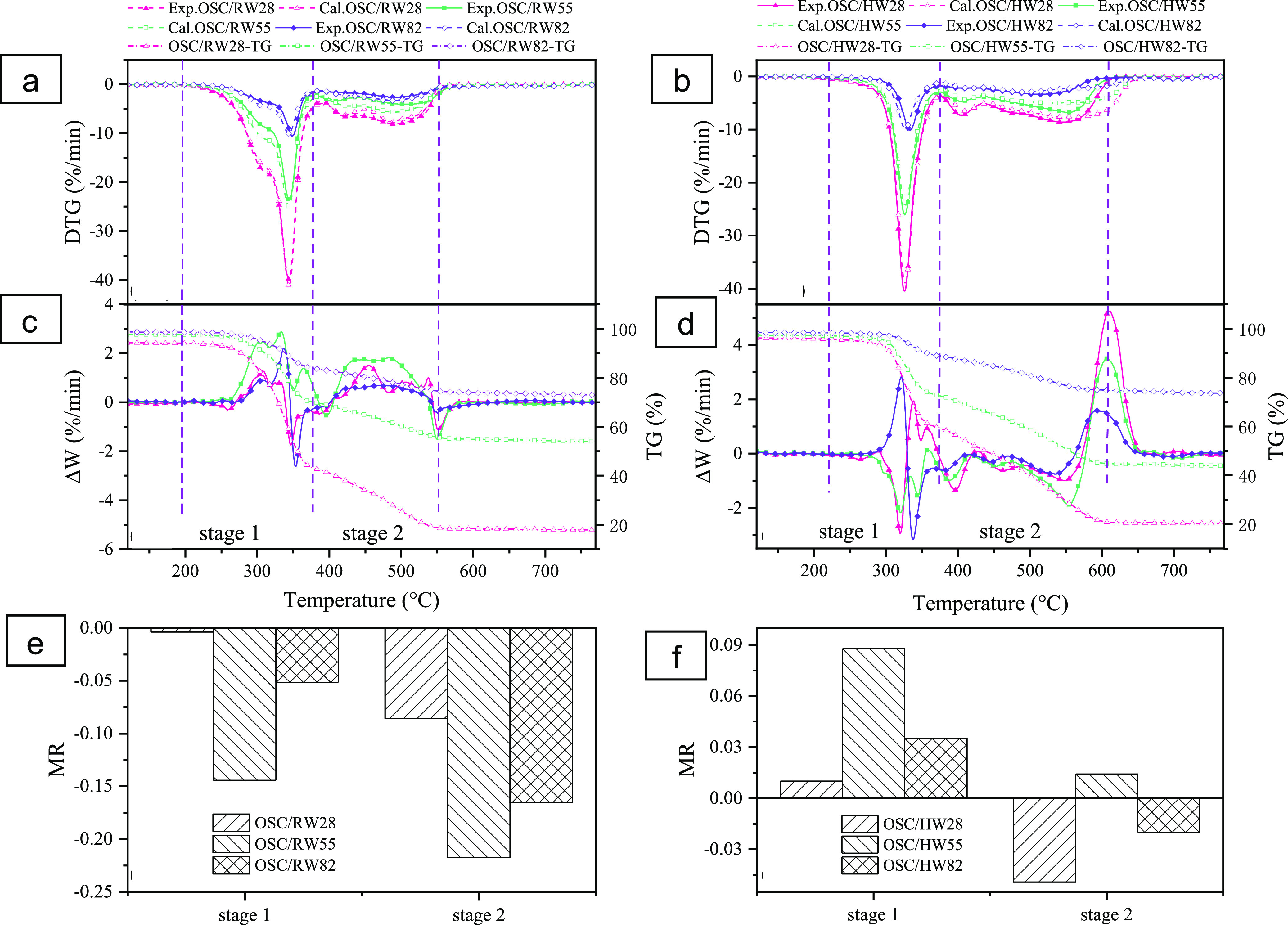
Experimental and calculated DTG curves and their deviations of the blends under different blending ratios: (a,b) OSC/RW; (c) (d) OSC/HW; (e) MR values of OSC/RW under different blending ratios; and (f) MR values of OSC/HW under different blending ratios.
2.4.2. Interaction between OSC and HW
As shown in Figure 2c, experimental curves of the weight loss rate were mostly below the calculated curves. It means that the experimental weight loss rate was larger than the predicted rate. Correspondingly, ΔW values were almost negative in stage 1 and stage 2, suggesting positive interaction for co-combustion (see Figure 2c). Notably, Figure 2d shows that the ΔW values were positive between 570 and 660 °C under different blending ratios, indicating a significant negative interaction. However, it should be noted that this largely negative interaction occurred at the end stage of co-combustion. The TG curve of OSC/HW blends, shown in Figure 2d, also indicated that the combustion process was almost completed when the temperature increased above 600 °C. It was consistent with the lower burnout temperatures of OSC/HW than that of HW (see Table 3 and Section 2.3). Consequently, it could be summarized that the co-combustion interaction between OSC and HW was mainly positive.
The contrast interaction between OSC/RW and OSC/HW was attributed to the modified properties of samples and partial removal of alkali metals after HTT (see Table 2). On the one hand, the HW surface became rougher than RW after HTT (see Figure S2). It accelerated the pore formation via the devolatilization process, which provided more gas diffusion channels to accelerate the decomposition rate, positively affecting the interactions between OSC and HW. A similar result was also obtained by Külaots et al.36 They found that the removing of AAEMs could open more pores and thereby provide active sites to the gaseous products. On the other hand, the lower contents of alkali metals in HW should be a disadvantage to co-combustion owing to less catalytic support. Positive interaction between OSC and HW would be discussed further in Section 2.6, according to kinetic analysis results.
2.5. Kinetic Analysis
2.5.1. Model-free Methods
Apparent activation energy (E) at a conversion ratio (α) from 0.2 to 0.8 with an interval step of 0.05 in stage 1 and stage 2 was determined. It is noted that the conversion ratio is not the overall conversion degree but the local conversion degree in each stage. The Arrhenius plots were depicted for stage 1 and stage 2 by Flynn–Wall–Ozawa (FWO) and Kissinger–Akahira–Sunose (KAS) methods (see Figures S3–S6 and Table S1). Table 5 lists the kinetic parameters based on the conversion ratio for each sample. The E values as a function of α are shown in Figure 5. The results indicated that the variation of E calculated by the FWO method had good agreement with those of KAS methods, verifying that the determined E values were consistent. As shown in Figure 3a,b, the E value of OSC gradually decreased in stage 1, whereas the E value reached a peak at α = 0.5 and increased again when α > 0.75 in stage 2. The variation of the E value was consistent with the thermal decomposition of OSC (see Section 2.2). For RW, one peak of the E value was observed at α = 0.3, and then, the E value decreased until α = 0.75 in stage 1. This stage could be attributed to the combustion of hemicellulose and cellulose. Hemicellulose was reported to have a higher E value than cellulose during thermal degradation, thus leading to such a change in the E value.21,37 After HTT, less amount of hemicellulose remained in HW compared to RW. Therefore, the initial E value of HW was lower than that of RW and continuously increased with α. When α > 0.6, the E value of HW was eventually larger than that of RW in stage 1, which was consistent with the composition profiles of their volatile and fixed carbon contents with increasing temperatures. The E values of RW and HW decreased with α in stage 2. In addition, HW had lower E than RW at any conversion ratio. This result agreed with previous studies.28,33 HTT degraded the highly cross-linked cell wall composed of cellulose, hemicellulose, and lignin, and thereby, the E value was decreased.
Table 5. Kinetic Triplets (E, A, and Model) for Samples at 40 °C/min by the Master Plot Method.
| sample | stage
1 |
stage
2 |
||||||
|---|---|---|---|---|---|---|---|---|
| Eavea | A | model | R2 | Eavea | A | model | R2 | |
| OSC | 128.65 | 1.08 × 10¹² | F2 | 0.999 | 172.44 | 3.03 × 10¹⁰ | R3 | 0.670 |
| RW | 211.33 | 1.80 × 10²⁰ | D4 | 0.998 | 169.28 | 4.12 × 10¹³ | D3 | 0.999 |
| OSC/RW28 | 212.26 | 8.00 × 10²⁰ | D2 | 0.999 | 177.34 | 1.30 × 10¹⁴ | D3 | 0.996 |
| OSC/RW55 | 207.90 | 3.43 × 10²⁰ | D2 | 0.997 | 163.61 | 8.86 × 10¹² | D3 | 0.996 |
| OSC/RW82 | 206.51 | 2.45 × 10²⁰ | D2 | 0.996 | 157.88 | 2.97 × 10¹² | D3 | 0.983 |
| HW | 208.40 | 2.47 × 10²¹ | F1 | 0.983 | 126.18 | 8.09 × 10⁹ | D3 | 0.998 |
| OSC/HW28 | 204.44 | 1.23 × 10²¹ | F1 | 0.983 | 145.40 | 2.57 × 10¹² | D3 | 0.997 |
| OSC/HW55 | 186.96 | 3.26 × 10¹⁹ | F1 | 0.981 | 151.16 | 6.01 × 10¹¹ | D3 | 0.998 |
| OSC/HW82 | 202.83 | 5.54 × 10²⁰ | F1 | 0.990 | 150.93 | 6.54 × 10¹¹ | D3 | 0.991 |
avergae E values (kJ/mol).
Figure 5.
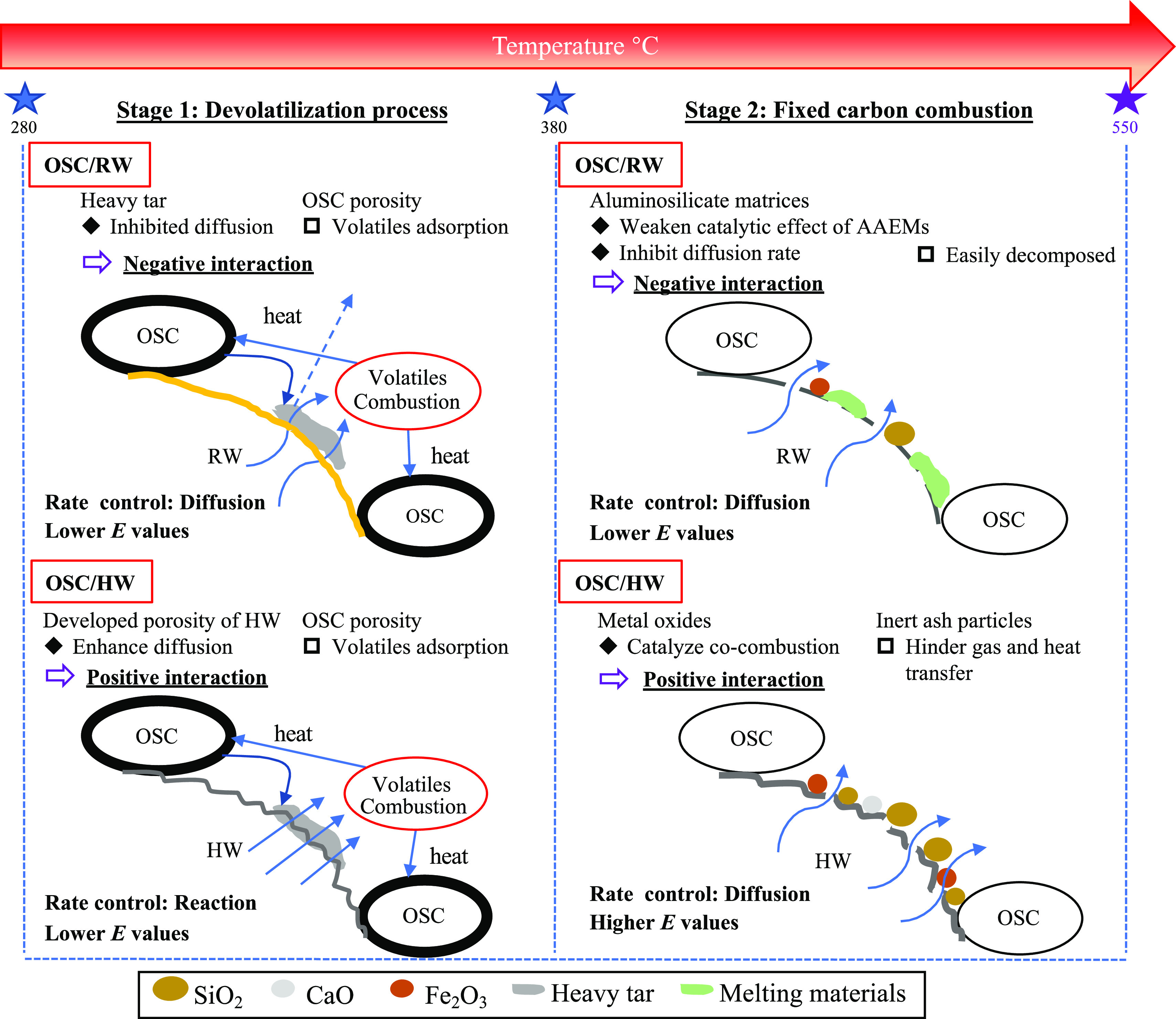
(Co-)combustion mechanism of OSC/RW and OSC/HW.
Figure 3.

Apparent activation energies (E) of OSC, RW, HW, and their respective blends: (a,b) variation of E for OSC, RW, and HW in stage 1 and stage 2; (c,d) variation of E for OSC/RW in stage 1 and stage 2; and (e,f) variation of E for OSC/HW in stage 1 and stage 2. S1: stage 1 and S2: stage 2.
As discussed in Section 2.2, the combustion stages (stage 1 and stage 2) of RW and HW had different temperature ranges compared with OSC but similar to those of OSC/RW and OSC/HW. It means that combustion stages of the blend co-combustion were mainly dominated by RW or HW. Therefore, we just analyzed the effect of OSC addition on the E values of OSC/RW and OSC/HW. The E values of the blends in stage 1 and stage 2 displayed similar trends to those of RW or HW. On the other hand, Figure 3c,e shows that the E values of OSC/RW and OSC/HW were lower than those of RW and HW in stage 1. Furthermore, the OSC addition significantly lowered the E values of OSC/HW, especially OSC/HW55. It agrees with the result in the previous section, in which OSC/HW55 displayed the strongest positive interaction in stage 1 (see Figure 2e). Figure 3d indicates that the E values of OSC/RW in stage 2 became lower with the increase in OSC proportion. However, the E values of OSC/RW shifted higher than RW when α > 0.75. Figure 3f indicates that the E values of OSC/HW gradually increased in stage 2 with OSC blending, implying that more energy input was required during co-combustion. It proposes that the OSC addition probably inhibited initializing the fixed carbon combustion of HW due to the accumulated ash layer when the combustion process continued. This result was not consistent with positive interactions to OSC/HW co-combustion (see Section 2.4.2). A similar phenomenon was also observed during the co-combustion of dyeing sludge and rice husk by Wang et al.38 They found that the E values of the blends were higher than those of individual samples regardless of positive interactions. Despite the inconsistence, either in stage 1 or stage 2, the E values of OSC/HW were significantly lower than those of OSC/RW under different OSC blending ratios.
2.5.2. Model-Based Methods
As shown in Figure 4, the average apparent activation energy, calculated from FWO and KAS methods, was used to establish experimental master plot curves of RW, HW, OSC, and their respective blends at 40 °C/min of heating rate. The curves of G(α) versus EP(u)/βR were plotted, and Table 6 lists the most feasible models of samples determined based on the linear least square. For RW, the α-dependent trends of P(u)/P(u0.5) had a good agreement with the D4 and D3 models in stage 1 and stage 2, respectively. It was consistent with previous studies.27 D3 and D4 are diffusion-based models which assume that diffusive transfer of gaseous products controls the overall reaction rate including numerous chemical reactions or microstructure changes in particles.27 For HW, the degradation curves in stage 1 and stage 2 were fitted to F1 and D3, respectively.
Figure 4.

P(u)/P(u0.5) versus α in stage 1 at 40 °C/min [(a) OSC, (c) RW and OSC/RW, and (e) HW and OSC/HW]; P(u)/P(u0.5) versus α in stage 2 at 40 °C/min [(b) OSC, (d) RW and OSC/RW, and (f) HW and OSC/HW]; and the direction of the pink dotted line arrow represented the variation of the curves with increasing OSC proportion in the blends.
Table 6. Most Frequently Used Models of Solid-State Processes.
| models | symbol | f(α) | G(α) |
|---|---|---|---|
| order of reaction | |||
| first order | F1 | 1 – α | –ln (1 – α) |
| second order | F2 | (1 – α)2 | (1 – α)−1 – 1 |
| third order | F3 | (1 – α)3 | [(1 – α)−2 – 1]/2 |
| diffusion | |||
| one-way transport | D1 | 0.5α | α2 |
| two-way transport | D2 | [−ln(1 – α)]−1 | (1 – α) ln(1 – α) + α |
| three-way transport | D3 | 1.5(1 – α)2/3 [1 – (1 – α)1/3]−1 | [1 – (1 – α)1/3]2 |
| Ginstling-Brounshtein equation | D4 | 1.5 [(1 – α)−1/3 – 1]−1 | (1 – 2α/3) – (1 – α)2/3 |
| limiting surface reaction between both phases | |||
| one dimension | R1 | 1 | α |
| two dimensions | R2 | 2(1 – α)1/2 | 1 – (1 – α)1/2 |
| three dimensions | R3 | 3(1 – α)2/3 | 1 – (1 – α)1/3 |
| exponential nucleation | |||
| power law, n = 1/2 | P2 | 2α1/2 | α1/2 |
| power law, n = 1/3 | P3 | 3α2/3 | α1/3 |
| power law, n = 1/4 | P4 | 4α3/4 | α1/4 |
| random nucleation and nucleus growth | |||
| two-dimensional | A2 | 2(1 – α) [ −ln(1 – α)]1/2 | [ −ln(1 – α)]1/2 |
| three-dimensional | A3 | 3(1 – α) [ −ln(1 – α)]2/3 | [ −ln(1 – α)]1/3 |
In stage 1 of OSC, the heavy components wrapped on the OSC surface were thermally evaporated and oxidized into sticky oils or tars with the increase in temperature.39 Hence, the rate-determining reaction was chemical reaction (F2) (see Figure 4a). However, Figure 4b indicates that the reaction models of OSC varied with the increase in α in stage 2. As α ranges from 0.2 to 0.4, the degradation profile of OSC showed the best agreement with R3 theoretical plots, a three-dimensional phase boundary reaction, which was regarded as the governing model in the combustion of carbonaceous materials.40 For OSC, heterogeneous reactions between the fixed carbon and nascent ash layer took place, and the surface area of ash became the limiting factor.41,42 When α > 0.4, the degradation curves of OSC sharply increased and could not locate into a specific reaction model. As shown in Figure 4c,e, the fittest models of OSC/RW (D2) and OSC/HW (F1) were similar to those of RW and HW in stage 1 under different OSC blending ratios. In stage 2, the degradation profiles of OSC/RW and OSC/HW still followed the D3 model, same as RW and HW (see Figure 4d,f). Notably, the degradation profiles of both OSC/RW and OSC/HW located between D3 and F3 and gradually approached F3 with increasing proportion of OSC. It is considered that OSC ash increased the surface area of the reactants and enlarged gas diffusion gaps. It might enhance gas diffusion during the fixed carbon combustion.42
2.6. Possible Mechanisms of OSC Co-combustion with RW or HW
Previous research confirmed that the intrinsic solids in OS had positive effects on the pyrolysis of OS,42,43 but the effect of solids on combustion and co-combustion with other feedstocks was still uncertain. The abovementioned sections revealed that the combustion of the blends contained complex reaction mechanisms. Therefore, in this section, these possible combustion mechanisms during the main (co-)combustion process (stage 1 and stage 2) were proposed based on the combustion characteristics, interactions, and kinetic analysis, with a schematic diagram depicted in Figure 5.
The devolatilization process at low-conversion stages of RW enhanced the formation of fixed carbon and heavy hydrocarbon layers. These layers conversely hindered the diffusion of gaseous products.40 Besides, highly ordered cellulose regions in RW acted as barriers and obstructed heat transfer from the external source.44 Therefore, the rate-limiting step in stage 1 was the diffusion reaction (D4). After HTT, the inorganic substances were partially leached out, and many strongly bonded compounds were cracked and removed, giving HW-improved homogeneity and well-developed pore structures. Heat transfer and gas diffusion inside HW particles became easier compared to RW, which enhanced gas diffusion. Thus, the rate-determination step was eventually shifted to F1.42 After blending with OSC, RW or HW ignited at first, and the released heat was consumed for OSC combustion. Meanwhile, the volatiles might be partially adsorbed by OSC due to its developed porosity (see Figure S2) and surface functional groups, leading to the reduction of the E values.45 These interactions should positively promote the decomposition rate of the blends. However, heavy components on the surface of OSC were thermally stimulated and accelerated the generation of sticky oils, which were inclined to coat the reactants (RW in this case) and conversely inhibited the diffusion.40 As a result, a negative interaction appeared between OSC and RW. On the other hand, the positive interaction between OSC and HW could be due to faster gas diffusion in HW according to the kinetic models (diffusion rate: F1 > D4). The volatiles from HW easily passed through owing to larger porosity of HW even when HW was coated by heavy components. Therefore, the positive interaction eventually remained.
In stage 2, the reaction model of RW was shifted from D2 in stage 1 to D3, representing a higher diffusion rate. This could be attributed to the enhanced pore structure during the devolatilization process, which provided channels for heat and gas transfer. However, with the removal of weakly bonded components, strongly bonded compounds in RW were recombined into hard solid polymers, impeding the diffusion reaction. Therefore, the dominant reaction model for HW became D3 in stage 2, signifying a lower diffusion rate than F1 in stage 1. For the blend co-combustion in stage 2, most of organic compounds in OSC were already evaporated and decomposed, eventually leaving a large amount of ash. The accumulated ash particles contained inert materials and could block the pore structure, which increased the thermal resistance of reactants. Hence, it made the E values of OSC/HW increase apparently with the increase in the OSC blending ratio. Besides, some metal oxides such as Fe2O3 and CaO in OSC ash were reported to pose catalytic effects during combustion.15 Cyclic deoxidation/oxidation reactions of these metal oxides assisted oxygen transfer to the carbon surface of HW and accelerated the diffusion rate.46 It promoted the decomposition and burnout of fixed carbon, which was consistent with decreased burnout temperature of OSC/HW. The catalytic support from metal oxides contained in OSC contributed to the positive interaction in OSC/HW co-combustion. For OSC/RW, low-melting-point substances, formed from reactions between alkali metals in RW and ash in OSC, were more susceptible to thermal decomposition than the inert ash particles, even though they aggravated the restriction on the decomposition rate. Therefore, OSC/RW exhibited decreasing E values with an increase in OSC addition, whereas with negative interactions due to inhibited diffusion.
3. Conclusions
The results indicated that RW or HW addition significantly improved conventional combustion parameters of OSC combustion and promoted the OSC harmless disposal efficiency. The RW blending caused negative interactions in co-combustion with OSC, although it decreased apparent activation energy. It mainly resulted from inhibited diffusion of volatile matters. In contrast, HW blending yielded positive interactions owing to developed porosity of HW, which effectively promotes volatiles diffusion, coupled with the catalytic support by metal oxides in OSC. Not only the catalytic effect of inorganic elements on co-combustion but also their physical influence on heat and volatiles transfers can contribute to improving co-combustion performance.
4. Materials and Methods
4.1. Sample Preparation
OS samples were supplied by Zhejiang Eco-Environmental Technology Co., Ltd, China. OSC samples were obtained by pyrolysis of OS. Pyrolysis experiments were performed in a vertical tube furnace, and details were outlined in the previous research.47 In each experiment, 20 g of OS was first placed in the pyrolysis reactor, and then, nitrogen gas was purged for 20 min to create an oxygen-free environment. Thereafter, the reactor was heated from room temperature to 450 °C at 10 °C/min and maintained for 20 min. When the heating process was finished, the reactor was naturally cooled to room temperature with the continuous nitrogen purge, and finally, the OSC was taken out and stored in a desiccator. Our previous research indicated that 450 °C was an optimal temperature for OS pyrolysis to obtain high-quality oil and save energy.43 Cherry blossom wood chips, purchased from a gardening market in Japan, were used as raw woody biomass (RW) samples due to the low moisture and high volatile content.
4.2. Sample Characterizations
All OSC, RW, and HW samples were crushed and sieved smaller than 200 μm for subsequent experiments. The proximate analysis and ultimate analysis results of OSC, RW, and HW are listed in Table 1. The higher heating values of samples were calculated using eq 4 which was developed by Francis and Lloyd48
| 4 |
where C, H, N, O, and S denoted the weight percentages of carbon, hydrogen, nitrogen, sulfur, and oxygen, respectively.
The ash composition of samples from XRF (S2 Ranger Bruker, Japan) analysis with the X-ray tube of the palladium anode is summarized in Table 2. The morphological surface characteristics of samples were observed via scanning electron microscopy (JSM-6510LA, JEOL Ltd., Japan) with an acceleration voltage of 6 kV.
For convenience, the blend of OSC and RW was named OSC/RW. OSC/HW represents the blend of OSC and HW. According to the blending ratio, OSC/RW blends were tagged as OSC/RW28 (20% OSC and 80% RW), OSC/RW55 (50% OSC and 50% RW), and OSC/RW82 (80% OSC and 20% RW). OSC/HW blends were also tagged as OSC/HW28, OSC/HW55, and OSC/HW82. As listed in Table 1, the HHV value of OSC was quite lower, resulting in the low efficiency of combustion treatment. In this study, the analyses of OSC/RW82 and OSC/HW82 were still performed for a comprehensive understanding of the interactive mechanisms during co-combustion, although the combustion efficiency was lower due to the high proportion of OSC.
4.3. Experimental Equipment and Methods
HTT experiments were conducted in a 400 mL stainless-steel reactor, and HTT steps were reported in detail previously.49 RW (6 g) and 60 g of pure water were mixed as raw samples. The hydrolysis of lignocellulose interfered with the carbonization process when the hydrothermal temperature was lower than 200 °C, whereas the hydrochar yield was reduced at a temperature above 250 °C.50 Therefore, the reaction temperature was set at 220 °C in this study.
Nonisothermal experiments were performed using a differential thermogravimetric analyzer (TA-60WS, Shimadzu, Japan). The sample (10 ± 0.5) was put on the bottom of an Al2O3 crucible and then set in the TGA analyzer with an empty Al2O3 reference for baseline calibration. The sample was heated from ambient temperature to 1000 °C under an air atmosphere at a 60 mL/min flow rate and different heating rates (5, 10, 40, and 50 °C/min). Each experiment was conducted twice or more for repeatability validation.
4.4. Combustion Performance Analysis
For combustion performance analysis, ignition temperature (Ti), burnout temperature (Tb), and peak temperature (Tmax) were obtained from the thermogravimetry and differential thermogravimetry (TG–DTG) curves. Ti was determined by the tangent method.51Tb and Tmax represented the temperature at a conversion rate of 98% and the maximum weight loss rate, respectively.52 Moreover, the ignition index (Di), burnout index (Db), and CCI were determined to evaluate the combustion performance of tested samples. These indexes were calculated using the following formulas (eqs 5–7)53
| 5 |
| 6 |
| 7 |
where Rp is the maximum weight loss rate (unit: %/min), Rmean is the average weight loss rate (unit: %/min), and ti, tp, tb, and Δt1/2 represent the ignition time, peak time, burnout time, and time interval between half values of Rp, respectively (unit: min).
4.5. Interaction Analysis
To evaluate the interactions between two blends during the co-combustion, the theoretical DTG curves were calculated based on their decomposition data and compared with experimental curves. The theoretical DTG curves were calculated using the average weight of the individual samples, according to eq 8
| 8 |
| 9 |
| 10 |
where DTGRW, DTGHW, and DTGOSC are the weight loss rate of RW, HW, and OSC, respectively (unit: %/min). The Xrw, Xhw, and Xosc are the proportion of RW, HW, and OSC in the blends, respectively (unit: %). The interaction index, ΔW, is the difference between the experimental and theoretical weight loss rate (unit: %/min). If ΔW < 0, it indicates a positive interaction for combustion at a specific temperature. The interaction index (MR: mean of the absolute error between experimental and calculated values divided by the mean of the calculated value) was used to analyze whether the interaction during the whole process is positive or not. If MR > 0, it represents a positive interaction; otherwise, it represents a negative interaction.
4.6. Kinetic Analysis
4.6.1. Introduction of Conventional Kinetic Analysis
The reaction rate of samples was described as54
| 11 |
where dα/dt is the conversion rate; α is the conversion degree; t is the reaction time; T is the reaction temperature; f(α) is the differential form of the reaction model; and k(T) is the rate constant relating to temperature and was determined using the Arrhenius equation54
| 12 |
where E, A, and R are the apparent activation energy, the pre-exponential factor, and the universal gas constant (8.314 J/(K·mol)), respectively.
The conversion degree of each stage was described as42
| 13 |
where ms, mt, and ms+1 are the initial weight, the weight at time t, and the final weight in a certain stage, respectively.
Combining eqs 11 and 12, the reaction rate could be transformed into
| 14 |
where β represents the heating rate and β = dT/dt.
Thereafter, eq 14 could be transferred into
| 15 |
where G(α) represents the integral form of the reaction function f(α), as exhibited in Table 6.
4.6.2. Model-free Methods
The isoconversional methods had been frequently used to estimate the reaction kinetics of solid fuels without referring to the reaction mechanism. In this study, the FWO method and KAS method were applied to calculate the apparent activation energy for combustion.
The FWO method was expressed as
| 16 |
The KAS method was described as
| 17 |
For a certain α, the apparent activation energy, E, was calculated depending on the slopes of the fitted straight line by plotting ln (β) versus 1/T for the FWO method and ln (β/T2) versus 1/T for the KAS method.
4.6.3. Master Plot Methods
In this study, the integral master plot method was employed to determine the kinetic model of various decomposition stages for samples. The starting decomposition rate of samples was slow, and thus, the conversion degree α was close to zero at the initial temperature T0, so eq 15 could be transferred as follows
| 18 |
where u = E/RT and P(u) was determined using the empirical equation P(u) = exp (−u)/u × (1.00198882u + 1.87391198).55 From isoconversional methods, the E value was estimated and used to determine a proper reaction model by simulating TG data. Taking α = 0.5 as a reference, eq 18 could be transformed into
| 19 |
where G(0.5) denoted the integral of the reaction model at α = 0.5, u0.5 = E/RT0.5, and T0.5 is the temperature at α = 0.5. Dividing eq 18 by eq 19, the integral master plots can be further converted to
| 20 |
On the left side of eq 20, the theoretical master plots, G(α)/G(0.5) versus α, were obtained from various G(α) functions. The experimental plots, P(u)/P(u0.5) versus α, were calculated from TG data and located on the right side of eq 20. By calculating the deviation between experimental plots and theoretical plots, the best fitted model was identified to determine the dominant combustion mechanisms of different samples.
Acknowledgments
The authors would like to appreciate financial supports by JSPS KAKENHI grant number 18H01567 and Chinese Scholarship Council (CSC).
Supporting Information Available
The Supporting Information is available free of charge at https://pubs.acs.org/doi/10.1021/acsomega.1c03944.
Combustion kinetic parameters of samples in stage 1 and stage 2 by FWO and KAS methods, Van Krevelen diagram of RW and HW, SEM images [RW, HW, and OSC], isoconversional plots at various conversion degrees in stage 1 by the FWO method, isoconversional plots at various conversion degrees in stage 1 by the KAS method, isoconversional plots at various conversion degrees in stage 2 by the FWO method, and isoconversional plots at various conversion degrees in stage 2 by the KAS method (PDF)
The authors declare no competing financial interest.
Supplementary Material
References
- Xu N.; Wang W.; Han P.; Lu X. Effects of ultrasound on oily sludge deoiling. J. Hazard. Mater. 2009, 171, 914–917. 10.1016/j.jhazmat.2009.06.091. [DOI] [PubMed] [Google Scholar]
- Hu G.; Li J.; Zeng G. Recent development in the treatment of oily sludge from petroleum industry: a review. J. Hazard. Mater. 2013, 261, 470–490. 10.1016/j.jhazmat.2013.07.069. [DOI] [PubMed] [Google Scholar]
- Cheng S.; Wang Y.; Fumitake T.; Kouji T.; Li A.; Kunio Y. Effect of steam and oil sludge ash additive on the products of oil sludge pyrolysis. Appl. Energy 2017, 185, 146–157. 10.1016/j.apenergy.2016.10.055. [DOI] [Google Scholar]
- Wang Z.; Gong Z.; Wang Z.; Fang P.; Han D. A TG-MS study on the coupled pyrolysis and combustion of oil sludge. Thermochim. Acta 2018, 663, 137–144. 10.1016/j.tca.2018.03.019. [DOI] [Google Scholar]
- Cheng S.; Zhang H.; Chang F.; Zhang F.; Wang K.; Qin Y.; Huang T. Combustion behavior and thermochemical treatment scheme analysis of oil sludges and oil sludge semicokes. Energy 2019, 167, 575–587. 10.1016/j.energy.2018.10.125. [DOI] [Google Scholar]
- Jiang X.; Han X.; Cui Z. New technology for the comprehensive utilization of Chinese oil shale resources. Energy 2007, 32, 772–777. 10.1016/j.energy.2006.05.001. [DOI] [Google Scholar]
- Golubev N. Solid oil shale heat carrier technology for oil shale retorting. Oil Shale 2003, 20, 324–332. [Google Scholar]
- Paul E.; Liu Y. Biological sludge minimization and biomaterials/bioenergy recovery technologies. Clean: Soil, Air, Water 2013, 41, 623. [Google Scholar]
- Anderson K.; Peters G. The trouble with negative emissions. Science 2016, 354, 182–183. 10.1126/science.aah4567. [DOI] [PubMed] [Google Scholar]
- Saidur R.; BoroumandJazi G.; Mekhilef S.; Mohammed H. A. A review on exergy analysis of biomass based fuels. Renewable Sustainable Energy Rev. 2012, 16, 1217–1222. 10.1016/j.rser.2011.07.076. [DOI] [Google Scholar]
- Sahu S. G.; Chakraborty N.; Sarkar P. Coal-biomass co-combustion: An overview. Renewable Sustainable Energy Rev. 2014, 39, 575–586. 10.1016/j.rser.2014.07.106. [DOI] [Google Scholar]
- Mandegari M.; Farzad S.; Görgens J. F. A new insight into sugarcane biorefineries with fossil fuel co-combustion: Techno-economic analysis and life cycle assessment. Energy Convers. Manage. 2018, 165, 76–91. 10.1016/j.enconman.2018.03.057. [DOI] [Google Scholar]
- McIlveen-Wright D. R.; Huang Y.; Rezvani S.; Mondol J. D.; Redpath D.; Anderson M.; Hewitt N. J.; Williams B. C. A techno-economic assessment of the reduction of carbon dioxide emissions through the use of biomass co-combustion. Fuel 2011, 90, 11–18. 10.1016/j.fuel.2010.08.022. [DOI] [Google Scholar]
- Lee S. H.; Lee T. H.; Jeong S. M.; Lee J. M. Economic analysis of a 600 mwe ultra supercritical circulating fluidized bed power plant based on coal tax and biomass co-combustion plans. Renewable Energy 2019, 138, 121–127. 10.1016/j.renene.2019.01.074. [DOI] [Google Scholar]
- Gong Z.; Wang Z.; Wang Z.; Fang P.; Meng F. Study on the migration characteristics of nitrogen and sulfur during co-combustion of oil sludge char and microalgae residue. Fuel 2019, 238, 1–9. 10.1016/j.fuel.2018.10.087. [DOI] [Google Scholar]
- Wang Z.; Gong Z.; Wang W.; Zhang Z. Study on combustion characteristics and the migration of heavy metals during the co-combustion of oil sludge char and microalgae residue. Renewable Energy 2020, 151, 648–658. 10.1016/j.renene.2019.11.056. [DOI] [Google Scholar]
- Lachman J.; Baláš M.; Lisý M.; Lisá H.; Milčák P.; Elbl P. An overview of slagging and fouling indicators and their applicability to biomass fuels. Fuel Process. Technol. 2021, 217, 106804. 10.1016/j.fuproc.2021.106804. [DOI] [Google Scholar]
- Zhang J.; Sun G.; Liu J.; Evrendilek F.; Buyukada M. Co-combustion of textile dyeing sludge with cattle manure: Assessment of thermal behavior, gaseous products, and ash characteristics. J. Cleaner Prod. 2020, 253, 119950. 10.1016/j.jclepro.2019.119950. [DOI] [Google Scholar]
- Wang Y.; Tan H.; Wang X.; Du W.; Mikulčić H.; Duić N. Study on extracting available salt from straw/woody biomass ashes and predicting its slagging/fouling tendency. J. Cleaner Prod. 2017, 155, 164–171. 10.1016/j.jclepro.2016.08.102. [DOI] [Google Scholar]
- Bach Q.-V.; Tran K.-Q.; Khalil R. A.; Skreiberg Ø.; Seisenbaeva G. Comparative assessment of wet torrefaction. Energy Fuels 2013, 27, 6743–6753. 10.1021/ef401295w. [DOI] [Google Scholar]
- Bach Q.-V.; Tran K.-Q.; Skreiberg Ø.; Khalil R. A.; Phan A. N. Effects of wet torrefaction on reactivity and kinetics of wood under air combustion conditions. Fuel 2014, 137, 375–383. 10.1016/j.fuel.2014.08.011. [DOI] [Google Scholar]
- Parshetti G. K.; Quek A.; Betha R.; Balasubramanian R. TGA–FTIR investigation of co-combustion characteristics of blends of hydrothermally carbonized oil palm biomass (EFB) and coal. Fuel Process. Technol. 2014, 118, 228–234. 10.1016/j.fuproc.2013.09.010. [DOI] [Google Scholar]
- Yao Z.; Ma X.; Lin Y. Effects of hydrothermal treatment temperature and residence time on characteristics and combustion behaviors of green waste. Appl. Therm. Eng. 2016, 104, 678–686. 10.1016/j.applthermaleng.2016.05.111. [DOI] [Google Scholar]
- Tong W.; Liu Q.; Ran G.; Liu L.; Ren S.; Chen L.; Jiang L. Experiment and expectation: Co-combustion behavior of anthracite and biomass char. Bioresour. Technol. 2019, 280, 412–420. 10.1016/j.biortech.2019.02.055. [DOI] [PubMed] [Google Scholar]
- Govindan B.; Chandra Babu Jakka S.; Radhakrishnan T. K.; Tiwari A. K.; Sudhakar T. M.; Shanmugavelu P.; Kalburgi A. K.; Sanyal A.; Sarkar S. Investigation on kinetic parameters of combustion and oxy-combustion of calcined pet coke employing thermogravimetric analysis coupled to artificial neural network modeling. Energy Fuels 2018, 32, 3995–4007. 10.1021/acs.energyfuels.8b00223. [DOI] [Google Scholar]
- Sezer S.; Kartal F.; Özveren U. The investigation of co-combustion process for synergistic effects using thermogravimetric and kinetic analysis with combustion index. Therm. Sci. Eng. Prog. 2021, 23, 100889. 10.1016/j.tsep.2021.100889. [DOI] [Google Scholar]
- Gil M. V.; Casal D.; Pevida C.; Pis J. J.; Rubiera F. Thermal behaviour and kinetics of coal/biomass blends during co-combustion. Bioresour. Technol. 2010, 101, 5601–5608. 10.1016/j.biortech.2010.02.008. [DOI] [PubMed] [Google Scholar]
- Yan W.; Perez S.; Sheng K. Upgrading fuel quality of moso bamboo via low temperature thermochemical treatments: dry torrefaction and hydrothermal carbonization. Fuel 2017, 196, 473–480. 10.1016/j.fuel.2017.02.015. [DOI] [Google Scholar]
- Ma P.; Yang J.; Xing X.; Weihrich S.; Fan F.; Zhang X. Isoconversional kinetics and characteristics of combustion on hydrothermally treated biomass. Renewable Energy 2017, 114, 1069–1076. 10.1016/j.renene.2017.07.115. [DOI] [Google Scholar]
- Munir S.; Daood S. S.; Nimmo W.; Cunliffe A. M.; Gibbs B. M. Thermal analysis and devolatilization kinetics of cotton stalk, sugar cane bagasse and shea meal under nitrogen and air atmospheres. Bioresour. Technol. 2009, 100, 1413–1418. 10.1016/j.biortech.2008.07.065. [DOI] [PubMed] [Google Scholar]
- Deng S.; Wang X.; Tan H.; Mikulčić H.; Yang F.; Li Z.; Duić N. Thermogravimetric study on the Co-combustion characteristics of oily sludge with plant biomass. Thermochim. Acta 2016, 633, 69–76. 10.1016/j.tca.2016.03.006. [DOI] [Google Scholar]
- Mlonka-Mędrala A.; Magdziarz A.; Gajek M.; Nowińska K.; Nowak W. Alkali metals association in biomass and their impact on ash melting behaviour. Fuel 2020, 261, 116421. 10.1016/j.fuel.2019.116421. [DOI] [Google Scholar]
- Zhang Y.; Zhang Z.; Zhu M.; Cheng F.; Zhang D. Interactions of coal gangue and pine sawdust during combustion of their blends studied using differential thermogravimetric analysis. Bioresour. Technol. 2016, 214, 396–403. 10.1016/j.biortech.2016.04.125. [DOI] [PubMed] [Google Scholar]
- Ma Q.; Han L.; Huang G. Potential of water-washing of rape straw on thermal properties and interactions during co-combustion with bituminous coal. Bioresour. Technol. 2017, 234, 53–60. 10.1016/j.biortech.2017.03.018. [DOI] [PubMed] [Google Scholar]
- Yao Z.; Ma X.; Wang Z.; Chen L. Characteristics of co-combustion and kinetic study on hydrochar with oil shale: a thermogravimetric analysis. Appl. Therm. Eng. 2017, 110, 1420–1427. 10.1016/j.applthermaleng.2016.09.063. [DOI] [Google Scholar]
- Külaots I.; Link S.; Arvelakis S.; Suuberg E. M.. Adsorption properties of wheat straw, reed and Douglas fir chars. International Carbon 2010 conference, 2010.
- Barzegar R.; Yozgatligil A.; Olgun H.; Atimtay A. T. TGA and kinetic study of different torrefaction conditions of wood biomass under air and oxy-fuel combustion atmospheres. J. Energy Inst. 2020, 93, 889–898. 10.1016/j.joei.2019.08.001. [DOI] [Google Scholar]
- Wang T.; Fu T.; Chen K.; Cheng R.; Chen S.; Liu J.; Mei M.; Li J.; Xue Y. Co-combustion behavior of dyeing sludge and rice husk by using TG-MS: Thermal conversion, gas evolution, and kinetic analyses. Bioresour. Technol. 2020, 311, 123527. 10.1016/j.biortech.2020.123527. [DOI] [PubMed] [Google Scholar]
- Liu C.; Liu J.; Sun G.; Xie W.; Kuo J.; Li S.; Liang J.; Chang K.; Sun S.; Buyukada M.; Evrendilek F. Thermogravimetric analysis of (co-) combustion of oily sludge and litchi peels: combustion characterization, interactions and kinetics. Thermochim. Acta 2018, 667, 207–218. 10.1016/j.tca.2018.06.009. [DOI] [Google Scholar]
- Yorulmaz S. Y.; Atimtay A. T. Investigation of combustion kinetics of treated and untreated waste wood samples with thermogravimetric analysis. Fuel Process. Technol. 2009, 90, 939–946. 10.1016/j.fuproc.2009.02.010. [DOI] [Google Scholar]
- Singh S.; Prasad Chakraborty J.; Kumar Mondal M. Intrinsic kinetics, thermodynamic parameters and reaction mechanism of non-isothermal degradation of torrefied Acacia nilotica using isoconversional methods. Fuel 2020, 259, 116263. 10.1016/j.fuel.2019.116263. [DOI] [Google Scholar]
- Qu Y.; Li A.; Wang D.; Zhang L.; Ji G. Kinetic study of the effect of in-situ mineral solids on pyrolysis process of oil sludge. Chem. Eng. J. 2019, 374, 338–346. 10.1016/j.cej.2019.05.183. [DOI] [Google Scholar]
- Cheng S.; Wang Y.; Gao N.; Takahashi F.; Li A.; Yoshikawa K. Pyrolysis of oil sludge with oil sludge ash additive employing a stirred tank reactor. J. Anal. Appl. Pyrolysis 2016, 120, 511–520. 10.1016/j.jaap.2016.06.024. [DOI] [Google Scholar]
- Poletto M.; Zattera A. J.; Santana R. M. C. Thermal decomposition of wood: Kinetics and degradation mechanisms. Bioresour. Technol. 2012, 126, 7–12. 10.1016/j.biortech.2012.08.133. [DOI] [PubMed] [Google Scholar]
- Gong Z.; Meng F.; Wang Z.; Fang P.; Li X.; Liu L.; Zhang H. Study on Preparation of an Oil Sludge-Based Carbon Material and Its Adsorption of CO2: Effect of the Blending Ratio of Oil Sludge Pyrolysis Char to KOH and Urea. Energy Fuels 2019, 33, 10056–10065. 10.1021/acs.energyfuels.9b02092. [DOI] [Google Scholar]
- Li X. G.; Ma B. G.; Xu L.; Luo Z. T.; Wang K. Catalytic Effect of Metallic Oxides on Combustion Behavior of High Ash Coal. Energy Fuels 2007, 21, 2669–2672. 10.1021/ef070054v. [DOI] [Google Scholar]
- Li S.; Cheng S.; Takahashi F.; Cross J. S. Upgrading crude bio-oil by in situ and ex situ catalytic pyrolysis through ZSM-5, Ni2Fe3, and Ni2Fe3/ZSM-5: Yield, component, and quantum mechanism. J. Renewable Sustainable Energy 2020, 12, 053101. 10.1063/5.0009689. [DOI] [Google Scholar]
- Cordero T.; Marquez F.; Rodriguez-Mirasol J.; Rodriguez J. J. Predicting heating values of lignocellulosics and carbonaceous materials from proximate analysis. Fuel 2001, 80, 1567–1571. 10.1016/s0016-2361(01)00034-5. [DOI] [Google Scholar]
- Khoshbouy R.; Takahashi F.; Yoshikawa K. Preparation of high surface area sludge-based activated hydrochar via hydrothermal carbonization and application in the removal of basic dye. Environ. Res. 2019, 175, 457–467. 10.1016/j.envres.2019.04.002. [DOI] [PubMed] [Google Scholar]
- He C.; Zhang Z.; Ge C.; Liu W.; Tang Y.; Zhuang X.; Qiu R. Synergistic effect of hydrothermal co-carbonization of sewage sludge with fruit and agricultural wastes on hydrochar fuel quality and combustion behavior. Waste Manage. 2019, 100, 171–181. 10.1016/j.wasman.2019.09.018. [DOI] [PubMed] [Google Scholar]
- Li X.-g.; Ma B.-g.; Xu L.; Hu Z.-w.; Wang X.-g. Thermogravimetric analysis of the co-combustion of the blends with high ash coal and waste tyres. Thermochim. Acta 2006, 441, 79–83. 10.1016/j.tca.2005.11.044. [DOI] [Google Scholar]
- Seggiani M.; Vitolo S.; Pastorelli M.; Ghetti P. Combustion reactivity of different oil-fired fly ashes as received and leached. Fuel 2007, 86, 1885–1891. 10.1016/j.fuel.2006.12.010. [DOI] [Google Scholar]
- Hurt R.; Gibbins J. Residual carbon from pulverized coal fired boilers:1. Size distribution and combustion reactivity. Fuel 1995, 74, 471–480. 10.1016/0016-2361(95)98348-i. [DOI] [Google Scholar]
- Vyazovkin S.; Burnham A. K.; Criado J. M.; Pérez-Maqueda L. A.; Popescu C.; Sbirrazzuoli N. ICTAC Kinetics Committee recommendations for performing kinetic computations on thermal analysis data. Thermochim. Acta 2011, 520, 1–19. 10.1016/j.tca.2011.03.034. [DOI] [Google Scholar]
- Tang W.; Liu Y.; Zhang H.; Wang C. New approximate formula for Arrhenius temperature integral. Thermochim. Acta 2003, 408, 39–43. 10.1016/s0040-6031(03)00310-1. [DOI] [Google Scholar]
Associated Data
This section collects any data citations, data availability statements, or supplementary materials included in this article.