A novel deep interval type-2 fuzzy LSTM (DIT2FLSTM) model applied to COVID-19 pandemic time-series prediction

Graphical abstract

Abstract

Currently, the novel COVID-19 coronavirus has been widely spread as a global pandemic. The COVID-19 pandemic has a major influence on human life, healthcare systems, and the economy. There are a large number of methods available for predicting the incidence of the virus. A complex and non-stationary problem such as the COVID-19 pandemic is characterized by high levels of uncertainty in its behavior during the pandemic time. The fuzzy logic, especially Type-2 Fuzzy Logic, is a robust and capable model to cope with high-order uncertainties associated with non-stationary time-dependent features. The main objective of the current study is to present a novel Deep Interval Type-2 Fuzzy LSTM (DIT2FLSTM) model for prediction of the COVID-19 incidence, including new cases, recovery cases, and mortality rate in both short and long time series. The proposed model was evaluated on real datasets produced by the world health organization (WHO) on top highly risked countries, including the USA, Brazil, Russia, India, Peru, Spain, Italy, Iran, Germany, and the U.K. The results confirm the superiority of the DIT2FLSTM model with an average area under the ROC curve (AUC) of 96% and a 95% confidence interval of [92–97] % in the short-term and long-term. The DIT2FLSTM was applied to a well-known standard benchmark, the Mackey-Glass time-series, to show the robustness and proficiency of the proposed model in uncertain and chaotic time series problems. The results were evaluated using a 10-fold cross-validation technique and statistically validated through the t-test method. The proposed DIT2FLSTM model is promising for the prediction of complex problems such as the COVID-19 pandemic and making strategic prevention decisions to save more lives.

1. Introduction

The COVID-19 pandemic was first reported in Wuhan in South China in early December 2019. The cause of the pandemic was later recognized as a novel coronavirus known as SAR-COV-2. As of November 2020, there have been 51,100,521 COVID-19 cases, with 1,324,714 deaths and 32,951,517 recovered cases. The U.S. had the highest number of COVID-19 death cases with 247,000 deaths [1], see Table 1 . During the last few months, several types of research have been conducted to realize the incidence of the disease and modelling uncertainties and prediction of the COVID-19 patterns during time series. The WHO is collecting and encouraging researchers to provide new methods and knowledge on COVID-19 and compiling it in a database to obtain a better strategy for handling this global issue. There are non-stationary time series features in Covid-19 pandemic patterns whose statistical attributes such as means and variances change over time. This study aims to model uncertainty sources associated with non-stationary time series features in real-world applications such as the COVID-19 pandemic.

Table 1.

Comparison of the New Cases, Death and recovered cases based on the WHO top 10 countries (7 Nov 2020).

Country	Population	Cases	Deaths	Recovered
USA	330,880,530	9.9 M	237 K	8.3 M
Brazil	212,463,372	5.7 M	163 K	5 M
Russia	145,930,700	1.75 M	31 K	1.3 M
India	1,379,122,578	8.4 M	126 K	8.2 M
UK	67,863,688	1.1 M	49 K	604 K
Peru	32,941,004	1 M	33 K	838 K
Spain	46,753,960	1.4 M	38 K	1.3 M
Italy	60,467,085	900 K	41 K	323 K
Iran	83,921,387	665 K	38 K	510 K
Germany	83,767,456	655 K	12 K	407 K

1.1. Literature review

This section presents an overview of data analytics and computational intelligence models applied to COVID-19 prediction.

In [2], the author described a bioinformatics inference system for modeling the SARS-CoV-2, which focuses on the design of a synthetic vaccine and a preventative peptidomimetic antagonist against the SARS-CoV- 2 with computer-aided techniques. In [3], the authors designed a framework for predicting the incidence of the COVID-19 pandemic based on the data transportation in China and applied machine learning methods for prediction of epidemic spread of Coronavirus driven by Spring Festival Transportation in time-series forecasting. In [3], [4], [5], population-based methods were proposed to predict the candidate targets. These methods used immune responses information through the sequence homology of the COVID-19 patterns. Also, the authors deliberated what could still be done to manage the COVID-19 pandemic with the standard measures of separation and contact tracing in risky countries. A computational spatial–temporal approach for modeling the distribution of SARS-CoV-2 in China was proposed in [6], [7] with a focus on culinary spice bioactive as potential therapeutics against sars-cov-2: computational investigation and data-driven modeling analysis. In [8], the authors proposed a propagation analysis method for modeling the time series. Their research proposed the transmission characteristics of the epidemic at different stages designed based on a Gaussian distribution theory to construct an innovative method of coronavirus transmission during a period.

On the other hand, in [9], [10], the authors describe various data mining and statistical techniques for predicting the COVID-19 pandemic in China with reasonable outcomes. They modeled an estimation of the daily number of new cases. Also, their proposed model emphasizes the control of the infection rates in short time-series. The authors in [11] proposed a deep LSTM approach to predict the SARS-CoV-2 new infection rates. They showed the trends of different countries and compared them to Canadian data to forecast the upcoming infections. They used LSTM to model the ending era of the pandemic in Canada for long time-series, but the challenge of non-optimal parameters in their model affected on the results of their work. Also, a computational intelligence framework for COVID-19 incidence based on a deep neural network technique and a social mimic tuning method associated with fuzzy logic and stacking methods in [12]. They described the dynamics of epidemic incidence of Coronavirus disease during a daily horizon. Also, in [13], the authors model a real-time prediction framework for the COVID-19 pandemic in a monthly format. These models were based on LSTM, convolutional neural network (CNN), and multi-layer perceptron neural nets using the dataset. Meanwhile, a novel SIR method has been proposed to model the pandemic incidence in Pakistan [14]. They projected the epidemic curve as realistic quarantine, social distancing, and probable medication scenarios in a short time-series.

In [15], [16], COVID-19 patients; however, they failed to use reasonable pandemic predictions and described a clinical SIR estimation method for modeling a time-series prediction of the COVID-19 new cases rates in a short time-series based on parameter approximation of time-dependent rates in China and Iran datasets. However, the main issue and limitation of their work is the lack of an appropriate dataset, which affects the reliability of their proposed model. In [17], [18], [19], [20], the authors proposed a dynamic model of the incidence of the viruses based on Auto-regressive integrated moving average (ARIMA), Transmission Dynamics Susceptible Latent Mild Critical Removed (SLMCR), Seasonal-ARIMA and the SIR model to predict the incidence of the COVID-19 in short time series.

The work presented in [21] predicted total cases in the most infected African countries with an ARIMA model in the short time-series. However, their proposed model does not consider the associated uncertainty in the procedure of forecasting. In [22], a comprehensive mathematical hybrid SIR and ARIMA were applied to predict the new cases in a short-term time series of the COVID-19 pandemic but using a limited number of cases in the dataset. Also, an intelligent hybrid ensemble artificial neural network with fuzzy inference aggregation was proposed in [23] for daily prediction of the COVID-19 incidence. Overall, the reviewed literature in this section, such as [15], [16], [21], cannot model the high-ordered uncertainty for the COVID-19 time-series forecasting. On the other hand, most of the related works in the kinds of literature were focused on the short time-series horizon, which is not suitable for strategic predictions. Also, most of the related works used a limited dataset in their model architecture which affects the reliability of their proposed approaches.

1.2. Challenges of the current intelligent methods

During the recent decade, applications of fuzzy logic systems, especially type-2 fuzzy systems in problems with high-order uncertainty, have been emerged, especially for predictions problems with dynamic and non-stationary problems [24]. Various types of research [25], [26], [27], [28] have been reported to model uncertainty using fuzzy set theory. Also, they have been applied to real-world applications through type-2 fuzzy logic systems, mostly in modeling uncertainty, control, and predictions [29], [30], [31]. Also, various neural network models such as recurrent neural networks (RNNs) have been applied to model and predict and model the time series data [11], [12], [32], [33], [34].

It has been proven that the RNNs, especially the LSTM network, have an excellent capability for solving complex problems. The LSTM model can learn the multi-layered inter-relationships between short and long time series [35], [36], [37]. The benefit of an LSTM cell compared to a regular recurrent unit is its cell memory [38]. The cell vector of an LSTM can capture the notion of forgetting part of its earlier stored memory and the part of its new information [39]. These capabilities can be used in the prediction of non-stationary problems [40]. In addition to the general benefits of using RNNs for time series prediction, the LSTM network can also automatically learn the temporal dependence from the data [41]. Hence, by definition, the LSTM has the capabilities of classical non-linear prediction methods to learn an arbitrary complex mapping from inputs to outputs. However, it cannot model the associated uncertainty in non-stationary features.

1.3. Highlights and structure of the article

• •This study takes advantage of type-2 fuzzy logic to develop a new architecture for handling high-order uncertainty in a deep time-series learning model.
• •A novel deep interval type 2 fuzzy LSTM (DIT2FLSTM) model has been proposed to predict non-stationary problems such as the COVOID-19 pandemic.
• •The proposed DIT2FLSTM model is capable for both short- and long time-series forecasting.

The rest of the article is ordered as follows: a theoretical research background has been presented in Section 2; the detailed structure and the mathematical model of the proposed DIT2FLSTM model have been denoted in Section 3; Section 4 presented the performance evaluation and comparison results of the proposed DIT2FLSTM based on ROC curve analysis and t-test statistical evaluation; Section 5 provides the discussion and the comparative results. The paper is concluded in Section 6.

2. Research background

This section presents a brief review of the LSTM network. Then, it follows by a review of interval type-2 fuzzy sets (IT2FS) concepts and the mathematic definitions.

2.1. A review of LSTM network

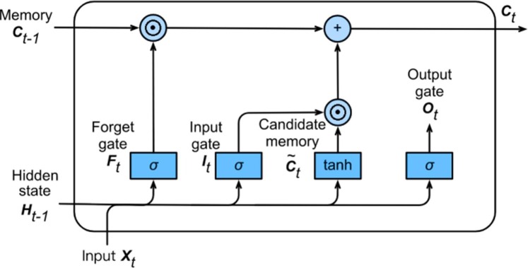
The LSTMs have been developed to address classic RNNs' limitations by enhancing the gradient vanishing in the network structure. The cell state$c_t$ in LSTM network stores the long-term information as follows [42]:

Input gate:

$$i_t=\sigma \left(W_{i1}{z}_{t-1}+W_{i2}{y}_t+W_{i3}{x}_t+W_{i4}s+b_i\right)$$ (1)

Output gate:

$$o_t=\sigma \left(W_{o1}{z}_{t-1}+W_{o2}{y}_t+W_{o3}{x}_t+W_{o4}s+b_o\right)$$ (2)

Forget Gate:

$$f_t=\sigma \left(W_{f1}{z}_{t-1}+W_{f2}{y}_t+W_{f3}{x}_t+W_{f4}s+b_f\right)$$ (3)

where $z_{t-1}$ is the hidden state of the LSTM at time $t-1$and $W$ are the weight matrices,   $t$  index is the time step, and $\sigma$ is the sigmoid activation function. Fig. 1 shows the architecture of the LSTM cell.

Fig. 1.

The architecture of the LSTM cell [42].

Also, the gates adjust the states and hidden cells of the LSTM using the following equations [42]:

Hidden state:

$$z_t=o_t\odot \mathrm{T}\mathrm{a}\mathrm{n}\mathrm{h}\left(c_t\right)$$ (4)

Cell state:

$$c_t=f_t\odot c_{t-1}+i_t\odot tanh(W_{c1}{z}_{t-1}+W_{c2}{y}_t+W_{c3}{x}_t+W_{c4}s+b_c)$$ (5)

where $\odot$ is the element-wise product, and $\mathit{tanh}$ is the activation function.

2.2. A review of interval Type-2 fuzzy Sets.

An interval type-2 fuzzy set represented as $\stackrel{}{A}$, is characterized through a type-2 MF ${\mu }_{\stackrel{}{A}(x,u)}$ where $x\in X$ and $u\in J_x\subseteq \left[0,1\right]$, [43],

$$\stackrel{}{A}=\left\{\left(\left(x,u\right),{\mu }_{\stackrel{}{A}\left(x,u\right)}\right)|\forall x\in X,\forall \in J_x\subseteq \left[0,1\right]\right\}$$ (6)

where ${0\le \mu }_{\stackrel{}{A}(x,u)}\le 1$, $X$is the domain of fuzzy set and $J_x$ is the domain of the secondary MF at $x$. $\stackrel{}{A}$ is as [46]:

$$\stackrel{}{A}=\frac{{\int }_{x\in X}{\int }_{u\in J_x}{\mu }_{\stackrel{}{A}}\left(x,u\right)}{x,u{J}_x}\subseteq \left[0,1\right]$$ (7)

where $\iint$ represents union overall admissible $x$ and $u$ [44].

$$\stackrel{}{A}=\frac{{\int }_{x\in X}{\int }_{u\in J_x}1}{x,u}=\frac{{\int }_{x\in X}\left[\frac{{\int }_{u\in J_x}1}{u}\right]}{x}$$ (8)

where $x$is the main variable, $J_x$, an interval in [0,1], is the primary MF of ×, u is the secondary variable, and ${\int }_{u\in J_x}$is the secondary MF at x.

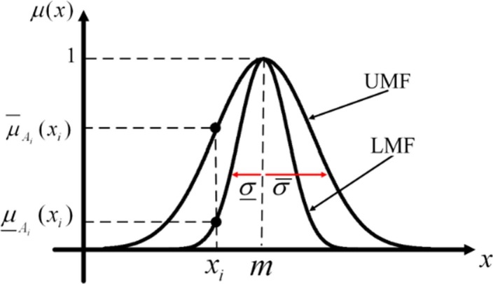
A FOU for a Gaussian primary MF with an uncertain standard deviation is shown in Fig. 2 . The FOU is bounded by an upper MF (UMF) ${\overline{\mu }}_{\stackrel{}{A}}\left(x\right)$and a lower MF (LMF) ${\underset{\_}{\mu }}_{\stackrel{}{A}}\left(x\right)$, which are type-1 fuzzy sets; consequently. Then, the uncertainty of $\stackrel{}{A}$is addressed by the union of all of the primary memberships, called the footprint of uncertainty (FOU) of $\stackrel{}{A}$ , i.e., $\left[FOU\stackrel{}{\left(A\right)}\right]$, [46] as:

$$\mathit{FOU}\stackrel{}{(A})=\bigcup _{x\in X}{J}_x$$ (9)

Fig. 2.

FOU for Gaussian primary membership function [46].

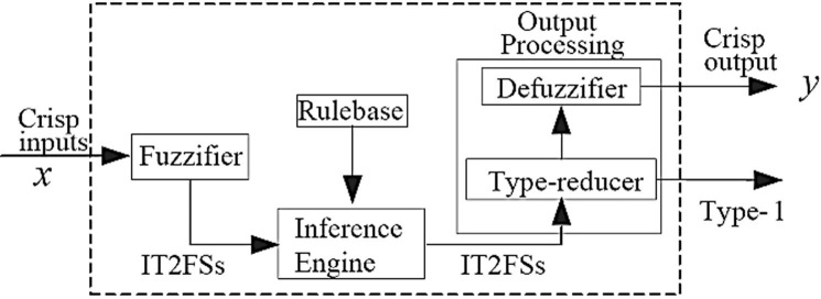
Also, the FOU in the IT2FLS provides more degree of freedom when designing a fuzzy system [48]. An interval type-2 fuzzy system (IT2FS) architecture contains four components. Fig. 3 shows the stricture and components of an IT2FLS.

Fig. 3.

The structure of the IT2FLS [47].

The TSK fuzzy rule type was considered in the proposed model, which has more precision than Mamdani rules [49]. In this work, the singleton fuzzifier was implemented [50], [51]. For defuzzification in the last step, the Karnik-Mendel (K.M.) algorithm [52] was applied. The following section presents the novel DIT2FLSTM model.

3. The proposed DIT2FLSTM model

This section presents the detailed architecture of the novel DIT2FLSTM model. In 3.1.2, the components of the DIT2FLSTM model are described. Then, in 3.2, the mathematical model of the DIT2FLSTM is presented. Finally, the cell structure of the proposed DIT2FLSTM has been discussed in 3.2.1.

3.1. The architecture of the DIT2FLSTM

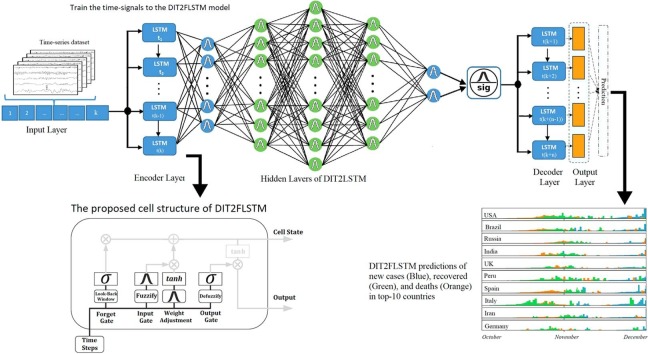
The structure of the proposed DIT2FLSTM and it’s layers have been illustrated in Fig. 4 . As shown in this architecture, the DIT2FLSTM is fuzzified using the IT2FS.

Fig. 4.

The architecture of the DFT2LSTM model.

Input Layer: The first layer is the input layer, which handles the original data in the input of the deep model. The output of the input layer can feed the inputs of the next layer, known as the hidden deep layers.

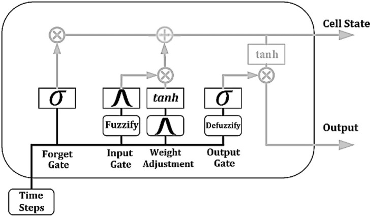
Encoder, Hidden, and Decoder layers: The main idea is mapping the entire input sequence to a vector and then using an encoder to generate the output sequence. In this layer, the encoder represents the entire input sequence in the hidden layer activities. The DIT2FLSTM model presents a novel cell structure in the encoder/decoder layer. The proposed structure can simply reform according to the dimension of the training time-series data set. The details are described in section 3.2.1 and shown in Fig. 5 .

Fig. 5.

The proposed cell structure of DIT2FLSTM.

Output Layer: The final layer is the prediction layer which decides and provides the final prediction based on the input features received from the previously hidden layers.

3.1.1. Components of the DIT2FLSTM model

Time series prediction models specify future values of a target $y_{\mathit{it}}$ for a given entity Xi at time t. The next step, prediction, is as follows:

$${\widehat{y}}_{i,t+1}=P_f\left(y_{i,t-e:t},x_{i,t-e:t},t\right)$$ (11)

where ${\widehat{y}}_{i,t+1}$is the predicted value in the next step, $y_{i,t-e:t}$ and $x_{i,t-e:t}$ are observations of the target and observed inputs, respectively, over a look-back window $e$, and $P_f$is the prediction function, and the final prediction is produced by $H_t$:

$$P_f\left(y_{i,t-e:t},x_{i,e-k:t},t,\right)=g_{\mathit{dec}}\left(H_t\right)$$ (12)

$$H_t=g_{\mathit{enc}}\left(y_{i,t-k:e},x_{i,t-e:t},t\right)$$ (13)

where $g_{\mathit{enc}}$ and $g_{\mathit{dec}}$ denote the encoder and decoder functions, respectively. The different parts of the LSTM network in the proposed DIT2FLSTM architecture are given by:

Definition 1

Let $N$ be the number of memory units of the model. In time-step$t$, i.e., the current time, the network keeps a set of vectors by the following equations:

$$i_t=\sigma \left(W_{\mathit{ix}}{x}_t+W_{\mathit{im}}{m}_{t-1}+W_{\mathit{ic}}{c}_{t-1}+b_i\right)$$ (14)

$$f_t=\sigma \left(W_{\mathit{fx}}{x}_t+W_{\mathit{fm}}{m}_{t-1}+W_{\mathit{fc}}{c}_{t-1}+b_f\right)$$ (15)

$$c_t=f_t\odot c_{t-1}+i_t\odot g(W_{\mathit{cx}}{x}_t+W_{\mathit{cm}}{m}_{t-1})$$ (16)

$$o_t=\sigma \left(W_{\mathit{ox}}{x}_t+W_{\mathit{om}}{m}_{t-1}+W_{\mathit{oc}}{c}_t+b_o\right)$$ (17)

$$m_t=o_t\odot h\left(c_t\right)$$ (18)

$$P_f=\phi \left(W_{\mathit{ym}}{m}_t+b_y\right)$$ (19)

where$\sigma$ is the sigmoid function, $W$ signifies the weight matrices, $W_{\mathit{ix}}$ is a matrix of fuzzy weights from the input cell to the output gate, $b$ signifies the bias vector, and $i,f,o,$and $c$ are the input gates, the hidden (forget) gate, the output gate, and cell activation function, $m$ is the cell output, and $\odot$ is the element-wise product, respectively. However, the hidden unit in this architecture is represented in memory blocks. Each block contains one or a large number of memory cells. This procedure allows these cells to preserve information for a particular time in an uncertain time series and decide which information needs to be stored and when to use it.

3.2. The mathematical model of the DIT2FLSTM

The input variables of the DIT2FLSTM model can be defined as p, $x_p$and$x_{p+1}$. Moreover, the Takagi Sugeno Kang (TSK) interval type-2 fuzzy inference is applied to describe the input structure of the model as follows:

$$p{\left\{\begin{array}{c}{R}_p^{j_1{j}_2}:if{x}_p={\stackrel{}{F}}_p^{j_1}\text{a}\text{n}\text{d}{x}_{t+1}={\stackrel{}{F}}_p^{j_2}\\ \text{t}\text{h}\text{e}\text{n}{y}_p=\left[{\underset{\_}{c}}_p^{j_1,j_2},{\overline{c}}_p^{j_1,j_2}\right]\end{array}\right\}}_{j_1,j_2=1}^M$$ (20)

where ${\stackrel{}{F}}_p^{j_1}$ and ${\stackrel{}{F}}_p^{j_2}$ are respectively the interval type-2 fuzzy sets of the inputs xp and xp + 1 in DIT2FLSTM, M is the number of applied fuzzy rules, ${\underset{\_}{c}}_i^{j_1,j_2}\mathrm{a}\mathrm{n}\mathrm{d}{\overline{c}}_i^{j_1,j_2}$ are the endpoints of a fuzzy rule $R_p^{j_1{j}_2}$ or the consequent. The product t-norm technique in Eq.20 is applied to compute the firing interval.

$$\left\{\begin{array}{c}{\underset{\_}{f}}^l\left({\mathbf{x}}^{\text{'}}\right)={\underset{\_}{\mu }}_{x_1^1}\left(x_1^{\text{'}}\right)\times \cdots \times {\underset{\_}{\mu }}_{x_p^{\text{'}}}\left(x_p^{\text{'}}\right)\\ {\overline{f}}^l\left({\mathbf{x}}^{\text{'}}\right)={\overline{\mu }}_{x_1^l}\left(x_1^{\text{'}}\right)\times \cdots \times {\overline{\mu }}_{x_p^{\text{'}}}\left(x_p^{\text{'}}\right)\end{array}\right)$$ (21)

The inference part of the DIT2FLSTM model can be entirely characterized by M fuzzy rules for inference process as:

$${\stackrel{}{R}}^l:if{x}_{1}is{\stackrel{}{F}}^l\cdots and{x}_{p}is{F}_p^l\mathrm{T}\mathrm{h}\mathrm{e}\mathrm{n}yis{\stackrel{}{G}}^l$$ (22)

where p is the inputs$x_1\in X_1,\cdots ,x_p\in X_p$ And the output y ∈ Y. The following equation represents the membership function as:

$${\mu }_{{\stackrel{}{R}}^l}\left(x,y\right)={\mu }_{\stackrel{}{A}\to {\widehat{G}}^l}\left(x,y\right)$$ (23)

where ∩ signifies the product t-norm operation [43]. The output of each fuzzy rule is ${\stackrel{}{B}}^l={\stackrel{}{A}}_x^{°}{\stackrel{}{R}}^l$, with membership functions of ${\mu }_{{\stackrel{}{B}}^l}\left(y\right)as$:

$${\mu }_{{\stackrel{}{B}}^l}\left(y\right)=\bigcup _{x\in X}\left[{\mu }_{A_x}\left(x\right)\cap {\mu }_{\stackrel{}{A}\to \overline{G}}\left(x,y\right)\right]$$ (24)

where ∘ represents the composition operation and ∪ signifies the maximum t-conorm operation [43], and ${\stackrel{}{F}}^l\left(\stackrel{´}{x}\right)$ denotes the firing interval for the fuzzy rule, where $x=\stackrel{´}{x}$ and $F^l$ is as:

$$F^l\left(x^{\text{'}}\right)\equiv \left[{\underset{\_}{f}}^l\left(x^{\text{'}}\right),{\overline{f}}^l\left(x^{\text{'}}\right)\right]$$ (25)

The firing output set ${\stackrel{}{B}}^l$ is produced through a fuzzy inference using ruleset and the aggregation of the consequent of as follows [44]:

$${\stackrel{}{B}}^l:\left\{\begin{array}{c}FOU\left({\stackrel{}{B}}^l\right)=\left[{\underset{\_}{\mu }}_{{\stackrel{}{B}}^{\text{'}}}\left(y\mid x^{\text{'}}\right),{\overline{\mu }}_{{\stackrel{}{B}}^{\text{'}}}\left(y\mid x^{\text{'}}\right)\right]\\ {\mu }_{{\stackrel{}{B}}^{\text{'}}}\left(y\mid x^{\text{'}}\right)={\underset{\_}{f}}^l\left(x^{\text{'}}\right)\ast {\underset{\_}{\mu }}_{{\stackrel{}{G}}^{\text{'}}}\left(y\right)\\ {\overline{\mu }}_{{\stackrel{}{B}}^{\text{'}}}\left(y\mid x^{\text{'}}\right)={\overline{f}}^l\left(x^{\text{'}}\right)\ast {\overline{\mu }}_{\widehat{G}}\left(y\right)\end{array}\right)$$ (26)

where ∗ represents the product t-norm operation. The final output ${\stackrel{}{B}}^l$ is obtained through the integration of all rule firing sets ${\stackrel{}{B}}^l$ on the output:

$${\stackrel{}{B}}^l:\left\{\begin{array}{c}\mathit{FOU}\left(\stackrel{}{B}\right)=\left[{\underset{\_}{\mu }}_{\stackrel{}{B}}\left(y\mid x^{\text{'}}\right),{\overline{\mu }}_{\stackrel{}{B}}\left(y\mid x^{\text{'}}\right)\right]\\ {\underset{\_}{\mu }}_{\stackrel{}{B}}\left(y\mid x^{\text{'}}\right)=\vee {\underset{\_}{\mu }}_{{\stackrel{}{B}}^M}\left(y\mid x^{\text{'}}\right)\\ {\overline{\mu }}_{\stackrel{}{B}}\left(y\mid x^{\text{'}}\right)=\vee {\overline{\mu }}_{{\stackrel{}{B}}^M}\left(y\mid x^{\text{'}}\right)\end{array}\right)$$ (27)

where ∨ represents the maximum operation. Then the type reduced set$Y_C\left(\stackrel{´}{x}\right)$ is obtained through computing the centroid $C_{\stackrel{´}{B}}$ of $\stackrel{}{B}$:

$$Y_C\left(x^{\text{'}}\right)=C_{\stackrel{}{B}}\left(x^{\text{'}}\right)=\frac{1}{\left[l_{\stackrel{}{B}}\left(x^{\text{'}}\right),r_{\stackrel{}{B}}\left(x^{\text{'}}\right)\right]}$$ (28)

where the two points $l_b\left(\stackrel{}{x}\right)$ and $r_b\left(\stackrel{}{x}\right)$ are computed through the K.M. algorithm in [45].

3.2.1. The DIT2FLSTM cell structure

In this research, the sigmoid squashing function was used on all the gates for the DIT2FLSTM cell structure as described follows:

$$\sigma =\frac{1}{{1+e}^{-x}}$$ (29)

The input of the cell uses the following equation:

$${\mathit{net}}_{c_{\left(t\right)}}=\sum W_{\phi j}y\left(t-1\right)$$ (30)

The input to the cell passes a non-linear function $f_{\phi }$, as follows:

$$f_{\phi }=\frac{4}{{1+e}^{-x}}-3$$ (31)

In the following equation, the main MFs for each antecedent are defined through Gaussian distribution with uncertain income as follows:

$${\mu }_k^i{(M}_{\left(k\right)})=\mathrm{e}\mathrm{x}\mathrm{p}\left[-\frac{1}{2}{\left[\frac{M_k-m_k^i}{{\sigma }_k^i}\right]}^2\right]$$ (32)

where $m_k^i\in \lfloor m_{k1}^i.m_{k2}^i\rfloor$ is the uncertain mean, k = 1,2 denotes the number of the antecedents, M denotes the number of the fuzzy rules, and ${\sigma }_k^i$ is the standard deviation. C in $n_c$ represents the number of memory cells in the training phase as follows:

$$n_r\times \left(3\times n_c\times n_o\right)$$ (33)

where $n_r$represents the number of rules in the inference engine of the fuzzy module and $n_o$is the number of outputs in the LSTM new cell and $n_c$represents the number of memory cells in the training phase. Furthermore, the values of the parameters by a ratio of $\frac{n_r}{n_c}$, and when $n_r<n_c$, the system can increase the model memory, denoted by $n_c$, which controls the number of parameters in the recurrent relations and the output layer in the proposed cell structure. The results are multiplied by the output of the gate unit. If the value is close to 0, then the output is not sent to the cell. The structure of the new cell in the DIT2FLSTM model is shown in Fig. 5.

Also, the input enters the cell whenever the input gate is activated. The cell state is defined as follows:

$$C_{\left(\mathrm{t}\right)}=i_t{C}_{(\mathrm{t}-1)}+i_t\left(t\right)+i_{t}g\left({\mathrm{net}}_{\mathrm{c}}\left(t\right)\right)$$ (34)

Then in the output gate of the cell is as follows:

$${\text{net}}_{{\text{out}}_j}\left(t\right)={\mathrm{\Sigma }}_m{w}_{{\text{out}}_{j}m}{y}^m\left(t-1\right)+\sum _{j=1}^{C_j}{w}_{{\text{out}}_j}{C}_{\left(\mathrm{t}\right)}$$ (35)

The activation function at the output gate is given by:

$$L=f_{\phi }\text{(}{\mathit{net}}_{{\mathit{out}}_j\left(t\right)})$$ (36)

where the cell output is ($y^c$) at the next step for prediction at time t as follows:

$$y^{\mathrm{c}}\left(t\right)={\mathit{net}}_{{\mathit{out}}_{\left(t\right)}}{c}_{\left(t\right)}$$ (37)

4. Performance evaluation and experiments

In this section, the DIT2FLSTM model was applied to an official dataset collected from the WHO official website. First, an ROC curve analysis of applying the DIT2FLSTM model to the official dataset is presented. Then a statistical evaluation of the DIT2FLSTM has been conducted to represent the model's capability for both short and long time-series predictions.

4.1. Applied data set on DIT2FLSTM model

The dataset contains the latest public data on the COVID-19 pandemic, including daily updates. This dataset includes detailed information about the number of confirmed cases, confirmed death, and confirmed recovery cases during the COVID-19 pandemic (February 2019 to November 2020).

4.2. An ROC curve analysis of the DIT2FLSTM model

In this section, an ROC curve analysis was conducted to have a reliable estimate of the performance of the DIT2FLSTM model, and the results were statistically verified as follows:

$$\text{Precision}=\frac{\mathit{TP}}{\left(TP+FP\right)}\times 100\%$$ (38)

$$\text{Recall}=\frac{\mathit{TP}}{(TP+TN)}\times 100\%$$ (39)

$$\text{F-Measure}=\frac{2{\text{"Precision}}^{\ast }\text{Recall}}{\text{Precision}+\text{Recall}}$$ (40)

$$\text{Accuracy}=\frac{\left(TP+TN\right)}{\left(TP+FP+FN+TN\right)}$$ (41)

$${\mu }_i=\frac{1}{10}\sum _{k=1}^{10}AUCj$$ (42)

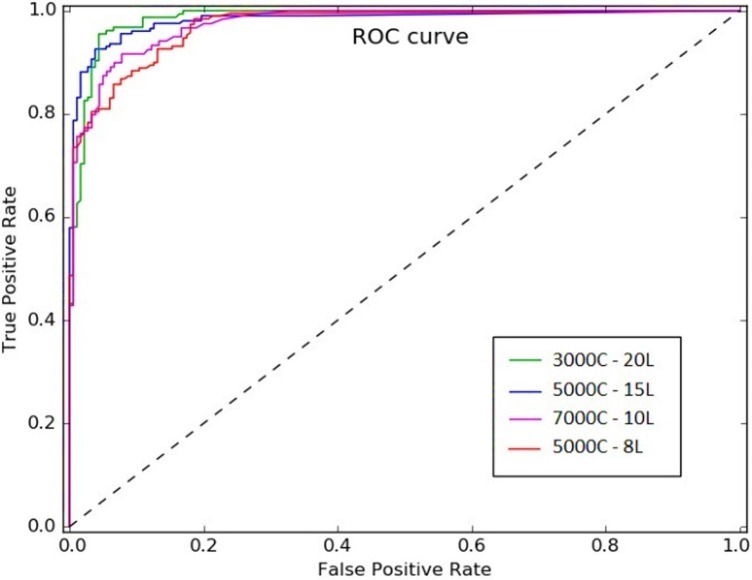
where ${\mu }_i$ is the means of the accuracy of the ROC curve for the 10-fold cross-validation. A 10-fold cross-validation technique was applied, randomly partitions the original sample into k equal sized subsamples. A single subsample is retained as the validation data for testing the model from the ten sub-samples, and the remaining nine are used as training data. This research was repeated ten times, while each subsample was used exactly once as validation test data. The obtained results of 10-fold cross-validation are reported in Table 2 . Table 3 presents the accuracy and the network size of the proposed DIT2FLSTM model based on various datasets for different network sizes, including various numbers of cells and depths of layers. The results reveal that the DIT2FLSTM withs 20 layers and 3000 cells were the most robust configuration, which reported the best performance during the prediction process as depicted in Fig. 6 .

Table 2.

10-fold cross-validation result of applying the DIT2FLSTM to the WHO top-10 incidence countries.

Fold #	USA	Brazil	Russia	India	UK	Peru	Spain	Italy	Iran	Germany
1	*91.88%	94.77%	97.67%	91.63%	90.65%	95.50%	95.67%	96.54%	94.76%	96.80%
2	90.25%	93.05%	92.29%	95.09%	95.88%	94.79%	94.92%	95.16%	91.08%	94.65%
3	90.12%	91.87%	95.98%	96.28%	93.67%	96.02%	91.84%	90.65%	90.87%	95.76%
4	91.19%	93.07%	92.08%	90.65%	93.16%	91.85%	92.56%	90.45%	92.90%	93.60%
5	92.89%	91.56%	95.03%	95.47%	92.03%	95.79%	93.73%	92.86%	94.55%	93.55%
6	90.93%	92.93%	97.86%	96.93%	95.73%	94.49%	91.98%	90.76%	96.00%	94.09%
7	93.69%	92.99%	93.78%	93.88%	94.59%	92.95%	94.92%	92.62%	94.67%	93.97%
8	94.18%	93.05%	95.79%	94.61%	93.29%	91.95%	92.00%	93.52%	94.90%	93.00%
9	93.59%	96.69%	94.87%	90.94%	92.68%	92.11%	93.15%	95.00%	92.45%	95.06%
10	94.87%	95.81%	92.23%	92.04%	94.77%	93.57%	94.65%	93.91%	93.75%	90.51%
Mean	92.35%	93.57%	94.75%	93.75%	93.64%	93.90%	93.54%	93.15%	93.59%	94.10%

^*The obtained accuracy is an average percentage of three cases, including new cases, recovery, and deaths in its fold number.

Table 3.

Training accuracy with different Cells and Layers of the proposed DIT2FLSTM.

Cell	Depth	Network Size	USA	Brazil	Russia	India	UK	Peru	Spain	Italy	Iran	Germany	Accuracy
10,000	8L	Underfit	87	86	84	82	81	85	89	90	86	90	84.16%
7000	10L	Underfit	82	84	80	82	82	84	86	90	88	92	82.33%
5000	15L	Overfit	95	96	98	96	94	95	93	92	92	94	95.66%
3000	20L	Fine Tuned	96	98	97	96	98	93	94	93	94	95	96.33%

Fig. 6.

ROC curve analysis for the DIT2FLSTM model.

4.3. Statistical evaluation of the DIT2FLSTM

In this section, the proposed DIT2FLSTM model was applied to both Mackey-Glass as a global benchmark and COVID-19 time series to show the proposed model's capability for predicting short and long time series. On the other hand, to perform a statistical evaluation of the performance of the proposed method, a t-test was conducted to validate the obtained results.

4.3.1. DIT2FLSTM applied on Mackey-Glass

This section presents the experimental results of applying the proposed DIT2FLSTM prediction method to the Mackey-Glass time series. The proposed DIT2FLSTM model was evaluated on a high-dimensional chaotic time-series system generated by the Mackey-Glass delay differential equations as follows:

$$\frac{\mathit{dx}\left(t\right)}{\mathit{dt}}=-0.1x\left(t\right)+\frac{0.2x\left(t-t_{\mathrm{\Delta }}\right)}{1+x{\left(t-t_{\mathrm{\Delta }}\right)}^{10}}$$ (43)

where $t_{\mathrm{\Delta }}$ is the delay of the time series. Furthermore, a statistical test was conducted on applying the DIT2FLSTM to the Mackey-Glass time series through t-test. First, we calculate the mean of observation as follows [53]:

$$t=\frac{\overline{X}-t_{\mathrm{\Delta }}}{s}\times \sqrt{n}$$ (44)

where, $\overline{X}$ is the sample mean, $t_{\mathrm{\Delta }}$ is the time delay mean, s is the sample size, and S is the standard deviation as follows [53]:

$$S=\sqrt{\frac{\sum _{i=1}^n{\left(X_i-\overline{X}\right)}^2}{n-1}}$$ (45)

Also, the RMSE was computed to assess the error of the DIT2FLSTM model in the Mackey-Glass time-series. The detailed calculation of RMSE is given by:

$$\mathit{RMSE}=\sqrt{\frac{1}{n}\sum _{i=1}^n{\left({\widehat{y}}^{\left(k\right)}-y^{\left(k\right)}\right)}^2}$$ (46)

where ${\widehat{y}}^{\left(k\right)}$ denotes the forecasted value, and $y^{\left(k\right)}$ is the actual value. Fig. 7 shows the statistical analysis of the DIT2FLSTM model on Mackey Glass time-series.

Fig. 7.

Statistical analysis of the DIT2FLSTM model for Mackey Glass time-series as a global benchmark.

Also, the obtained results showed that the minimum error of the DIT2FLSTM model was 0.00251, and the average error was 0.00301. Table 4 shows the quantitative comparison of DIT2FLSTM uncertainty in Mackey-Glass and COVID-19 datasets.

Table 4.

Comparison of DIT2FLSTM in Mackey-Glass and COVID-19.

Samples	Mackey Glass			COVID-19
	RMSE	STD	Mean	RMSE	STD	Mean
100	1.2672	0.0351	0.127	0.1021	1.2672	0.097
1000	0.9821	0.0267	0.086	0.0537	0.9821	0.076
5000	0.5231	0.0171	0.089	0.0315	0.5231	0.071
10,000	0.2176	0.0149	0.084	0.0208	0.2176	0.044

4.3.2. Null hypothesis and left tailed t-test

In this section, a two-sample t-test (left tailed) has been conducted. The null hypothesis was defined as [54], [55]: H₀ = ${\mu }_i>{\mu }_j$and, H₁: ${\mu }_i<{\mu }_j$, where ${\mu }_i$ and ${\mu }_j$ are the means of the area under the ROC curve (AUC) of DIT2FLSTM and IT2FLS for ten different iterations of 10-fold cross-validation assessment. The obtained results of the t-test analysis are shown in Table 5 , which demonstrates the advantage of the proposed DIT2FLSTM method for COVID-19 time-series prediction compared to the IT2FLS. The obtained results in Table 5 shows that the t-test failed to reject the null hypothesis.

Table 5.

Left-tailed T-test analysis of the DIT2FLSM and IT2FLS.

Fold#	DIT2FLSTM	IT2FLS
1	0.9071	0.7434
2	0.9212	0.7291
3	0.9252	0.6359
4	0.8905	0.6301
5	0.9421	0.7218
6	0.9312	0.7925
7	0.9651	0.7651
8	0.9426	0.7271
9	0.9667	0.8112
10	0.9821	0.8214
Mean	0.9673	0.8277

4.4. Comparison analysis of the results

In this section, Table 6 presents a comparison of conventional methods and the proposed DIT2FLSTM model. According to the obtained results, the proposed DIT2FLSTM model has reported the highest performance compared to the counterpart models, including the LSTM, IT1FLS, IT2FLS, T1FLSTM, and T2ANFIS for the COVID-19 time-series prediction.

Table 6.

Comparison of conventional methods and DIT2FLSTM model.

Method	AUC%	CI%	Recall	Precision	F-1
IT1FLS	79.23	[77–81]	78.52%	79.67%	80.33%
IT2FLS	82.07	[80–85]	81.23%	82.41%	82.77%
LSTM	90.92	[87–92]	91.79%	92.24%	90.33%
Fuzzy-LSTM	92.05	[88–93]	91.76%	92.27%	91.17%
IT2ANFIS [30]	91.21	[89–93]	92.15%	91.15%	90.53%
DIT2FLSTM	96.00	[92–97]	96.17%	95.83%	95.26%

Meanwhile, the time-series complexity was determined by the number of computational steps needed to run the algorithm of the DIT2FLSTM as a function for several data samples as the input size. Time measurement was computed by order of the models and consumption, including the hour, minute, and seconds (00:00:00) as shown in Table 7 , where N is the number of instructions and M  is the input size.

Table 7.

Complexity Comparison of DIT2FLSTM and counterparts.

Model	Order	Time Consumption
IT1FLS	O(1) + O(N)	0:00:32
IT2FLS	O(N) + O(M*N)	0:00:48
LSTM	O(1) + O(M*N)	0:00:42
T1-LSTM	O(1) + O)log(M*N)(	0:01:13
T2-ANFIS [30]	(4*O(1) + O(N2))	0:01:34
DIT2FLSTM	(6*O(1) + O(N*M) + O(N2)	0:01:43

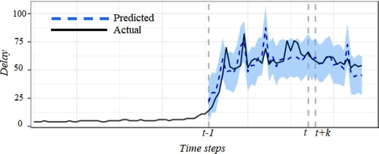
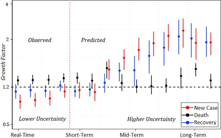
Fig. 8 illustrates the cumulative representation of the COVID-19 prediction. This figure shows the associated uncertainty in prediction of the new case, death, and recovery for COVID-19 time-series.

Fig. 8.

Illustrations of associated uncertainty in different time steps.

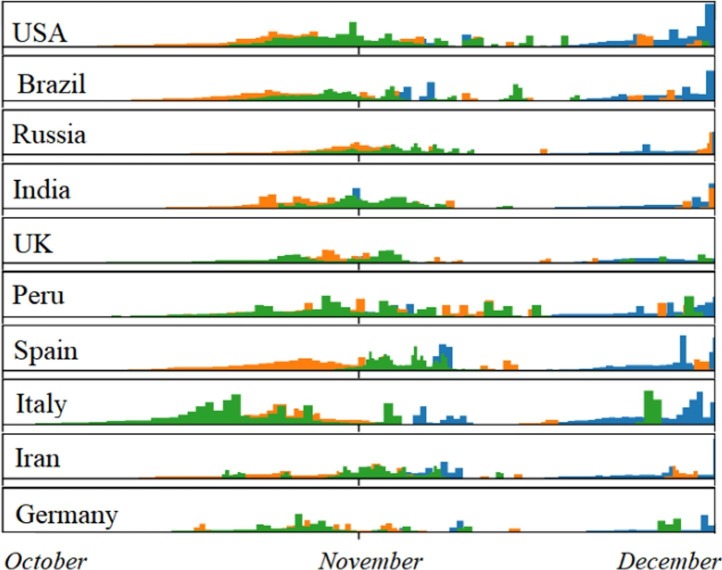
The prediction results of the 10-top countries based on the proposed DIT2FLSTM model are shown in Fig. 9 . Also, in the final part of this section, the DIT2FLSTM model has been compared to related works in Table 8 .

Fig. 9.

DIT2FLSTM predictions of new cases (Blue), recovered (Green), and deaths (Orange) in top-10 countries. (For interpretation of the references to colour in this figure legend, the reader is referred to the web version of this article.)

Table 8.

A comparison of the DIT2FLSTM model and related works.

Methodology	Prediction Factor	Horizon
Time-dependent dynamic SIR [14]	New cases	Daily
Generalized Additive SIR [16]	Death cases	Daily
Transmission Dynamics Susceptible-Latent-Mild-Critical-Removed (SLMCR) [18]	New cases	Monthly
Modified SEIRD with ARIMA and Transition Dynamic [19]	Susceptible, Exposed, Infective, Recovered, Death	Daily
ARIMA (Auto-Regressive Integrated Moving Average) [20]	Confirmed Cases	Daily
Fuzzy Arima [21]	Recovery cases	Daily
Hybrid Sir-ARIMA [22]	New cases	Daily
LSTM network [11]	New cases	Weekly
Neuro-fuzzy [23]	New cases	Daily
DIT2FLSTM	New cases, death, and recovery	Daily and Monthly

5. Discussion

Experimental results revealed that the proposed DIT2FLSTM model had reported reliable results based on the real COVID-19 datasets obtained from the official WHO websites. Moreover, the ROC curve analysis shows 96% (AUC) performance for the DIT2FLSTM model for COVID-19 prediction on the WHO dataset. The experimental results revealed that the performance of the proposed DIT2FLSTM model was better than its counterparts; i.e.,17% greater than T1FLS, 14% greater than IT2FLS, 6% greater than LSTM, 4% greater than T1FLSTM, and 5% better than the IT2ANFIS, in terms of the AUC. The proposed DIT2FLSTM model has an average AUC of 96% with a 95% confidence interval [92–97] % to predict the mortality rate of the COVID-19 pandemic. Also, to show the proficiency of the proposed DIT2FLSTM, a Mackey-Glass-time series with a delay equation was applied. The minimum error of the DIT2FLSTM model was 0.00251, where the average error was 0.00301 in terms of the RMSE.

This research presents the DIT2FLSTM model for predicting the COVID-19 time series as a real-world challenge. However, the capability of the proposed model is not limited to this specific application. Furthermore, the proposed DIT2FLSTM model has the potential to be applied to other biomedical applications, including biopharmaceutical and clinical studies in horizon of time series.

6. Conclusion

In this study, a novel DIT2FLSTM model was proposed to predict the incidence of new cases, recovery cases, and mortality rates of the COVID-19 pandemic. The proposed DIT2FLSTM model was applied to the WHO global dataset. The proposed DIT2FLSTM model can be applied to the uncertain and chaotic time series for short and long time series prediction. The obtained results show that the proposed DIT2FLSTM model is proficient at coping with the uncertainty to model phenomena such as the COVID-19 pandemic. Additionally, the model can easily get updated when new cases are reported because of its deep architecture. Further studies are suggested for tuning the DIT2FLSTM cell structure parameters and applying them to other real-world applications associated with non-stationary uncertainties. The optimization techniques such as evolutionary algorithms can be applied to improve the performance of the DIT2FLSTM model.

CRediT authorship contribution statement

Aref Safari: Conceptualization, Methodology, Visualization, Investigation, Validation, Programming, Writing- Original draft preparation. Rahil Hosseini: Supervision, Methodology, Validation, Writing preparation, Reviewing, Editing. Mahdi Mazinani: Consultant, Reviewing.

Declaration of Competing Interest

The authors declare that they have no known competing financial interests or personal relationships that could have appeared to influence the work reported in this paper.

Appendix A.

The notations, petameter, and the variables of the proposed DIT2FLSTM model are summarized and described in Table 9 .

Table 9.

Notations for the components of the DIT2FLSTM model.

No	Notation	Petameter and variables
1	$i_t$	Input gate at time t
2	$o_t$	Output gate at time t
3	$f_t$	Hidden (forget) gate at time t
4	$g_{\mathit{enc}}$	Encoder function
5	$g_{\mathit{dec}}$	Decoder function
6	$f_{\phi }$or$\sigma$	Activation function (Sigmoid)
7	$\odot$	element-wise product
8	$\mathit{tanh}$	Hyperbolic tangent
9	$U$	The hidden layer weight matrix
10	$W$	Wight metric
11	$W_{\mathit{ix}}$	Input weight matrix
12	e	Look-back window
13	$Z_t$	Hidden cell at time t
14	$Z_{t-1}$	Hidden cell state at time t-1
15	t	Timestep
16	b	Bias
17	${\stackrel{}{F}}_p$	Interval type-2 fuzzy set for input p
18	$R_p$	The fuzzy rule for input p
19	${\stackrel{}{F}}^l\left(\stackrel{´}{x}\right)$	Firing interval of fuzzy rule
20	$c_i^{j_1,j_2}$	endpoints of the consequent of a rule in cell
21	${\mu }_{{\stackrel{}{R}}^l}$	The MF of the rule in a cell
22	∩	t-norm
23	${\stackrel{}{B}}^l$	The output of the fuzzy rule
24	∘	composition operation
25	∪	t-conorm
26	∗	Product t-norm
27	$\vee$	Maximum operations
28	$Y_C$	Type-redacted of cell output
29	$l_b$	Left boundary
30	$r_b$	Right boundary
31	k	Number of Antecedent
32	${\mathit{net}}_{\mathit{cj}}$	The input of a cell
33	$y^{\mathrm{c}}$	The output of a cell
34	${\mathit{net}}_{{\mathit{in}}_j}$	Net of an input gate
35	${\mathit{net}}_{{\phi }_j}$	Net of a forget gate
36	${\mathit{net}}_{{\mathit{out}}_j}$	Net of an output gate
37	$C$	Number of the memory cell
38	$c_t$	Cell state at time t
39	m	Mean
40	N	Number of memory units
41	L	activation function at output gate

Appendix B. Supplementary data

The following are the Supplementary data to this article:

References

- 1.Hoseinpour Dehkordi A., Alizadeh M., Derakhshan P., Babazadeh P., Jahandideh A. Understanding epidemic data and statistics: A case study of COVID-19. J. Med. Virol. 2020;92(7):868–882. doi: 10.1002/jmv.25885. [DOI] [PMC free article] [PubMed] [Google Scholar]
- 2.B. Robson, Computers and viral diseases. Preliminary bioinformatics studies on the design of a synthetic vaccine and a preventative peptidomimetic antagonist against the SARSCoV- 2 (2019-nCoV, COVID-19) coronavirus, Comput. Biol. Med. 119, 103670 (2020). http://doi.org/10.1016/j.compbiomed.2020.103670. [DOI] [PMC free article] [PubMed]
- 3.Fan C., Liu L., Guo W., Yang A., Ye C., Jilili M., Ren M., Xu P., Long H., Wang Y. Prediction of Epidemic Spread of the 2019 Novel Coronavirus Driven by Spring Festival Transportation in China: A Population-Based Study. Int. J. Environ. Res. Public Health. 2020;17(5) doi: 10.3390/ijerph17051679. [DOI] [PMC free article] [PubMed] [Google Scholar]
- 4.Goh GK, Dunker AK, Foster JA, Uversky VN, Rigidity of the Outer Shell Predicted by a Protein Intrinsic Disorder Model Sheds Light on the COVID-19 (Wuhan-2019-nCoV) Infectivity. Biomolecules. 10(2) (2020). http://doi.org/10.3390/biom10020331. [DOI] [PMC free article] [PubMed]
- 5.Grifoni, A, Sidney, J, Zhang, Y. Scheuermann, B. Sette, A, A Sequence Homology and Bioinformatic Approach Can Predict Candidate Targets for Immune Responses to SARS-CoV-2. Cell. Host. Microbe, 27(4) (2020) 671-680. http://doi.org/10.1016/j.chom.2020.03.002. [DOI] [PMC free article] [PubMed]
- 6.Jagadish Natesh, Priya Mondal, Dhanamjai Penta, Abdul Ajees Abdul Salam, Syed Musthapa Meeran, Culinary spice bioactives as potential therapeutics against SARS-CoV-2: Computational investigation, Comput. Biol. Med., 128 (2020). http://doi.org/10.1016/j.compbiomed.2020.104102. [DOI] [PMC free article] [PubMed]
- 7.Huang R., Liu M., Ding Y. Spatial-temporal distribution of COVID-19 in China and its prediction: A data-driven modeling analysis. J. Infect. Dev. Ctries. 2020;14(3):246–253. doi: 10.3855/jidc.12585. [DOI] [PubMed] [Google Scholar]
- 8.Lixiang Li, Zihang Yang, Zhongkai Dang, Cui Meng, Jingze Huang, Haotian Meng, Deyu Wang, Guanhua Chen, Jiaxuan Zhang, Haipeng Peng, Yiming Shao, Propagation analysis and prediction of the COVID-19, Infectious Disease Modelling, 5 (2020) 282-292. http://doi.org/10.1016/j.idm.2020.03.002. [DOI] [PMC free article] [PubMed]
- 9.Li Q., Feng W. Trend and forecasting of the COVID-19 outbreak in China. J. Infect. 2020;80:469–496. doi: 10.1016/j.jinf.2020.01.017. [DOI] [PMC free article] [PubMed] [Google Scholar]
- 10.Liu, Z, Magal, P. Seydi, O. Webb, G. Understanding Unreported Cases in the COVID-19 Epidemic Outbreak in Wuhan, China, and the Importance of Major Public Health Interventions. Biology, 9(3) (2020). http://doi.org/10.3390/biology9030050. [DOI] [PMC free article] [PubMed]
- 11.Chimmula V., Zhang L. Time series forecasting of COVID-19 transmission in Canada using LSTM networks, Chaos. Solitons & Fractals. 2020;135 doi: 10.1016/j.chaos.2020.109864. [DOI] [PMC free article] [PubMed] [Google Scholar]
- 12.Mesut Toğaçar, Burhan Ergen, Zafer Cömert, COVID-19 detection using deep learning models to exploit Social Mimic Optimization and structured chest X-ray images using fuzzy color and stacking approaches, Comput. Biol. Med., 121 (2020). http://doi.org/10.1016/j.compbiomed.2020.103805. [DOI] [PMC free article] [PubMed]
- 13.Marzouk M., Elshaboury N., Abdel-Latif A., Azab S. Deep learning model for forecasting COVID-19 outbreak in Egypt. Process Saf. Environ. Prot. 2021;153:363–375. doi: 10.1016/j.psep.2021.07.034. [DOI] [PMC free article] [PubMed] [Google Scholar]
- 14.M. Waqas, M. Farooq, R. Ahmad, and A. Ahmad, Analysis and Prediction of COVID-19 Pandemic in Pakistan using Time-dependent SIR Model, COVID-19 research community. 14 (2020). http://doi.org/10.1080/17513758.2020.1814883.
- 15.Q. Lina, S. Zhaob, D. Gaod, Y. Loue, S. Yangf, S. S. Musae, M. H. Wangb, Y. Caig, W. Wangg, L. Yangh, D. Hee, A conceptual model for the coronavirus disease 2019 (COVID-19) outbreak in Wuhan, China with individual reaction and governmental action, Int. J. Infect. Dis., 93 (2020) 211-216. http://doi.org/10.1016/j.ijid.2020.02.058. [DOI] [PMC free article] [PubMed]
- 16.Chen Y.C., Lu P.E., Chang C.S., Liu T.H. A Time-dependent SIR model for COVID-19 with Undetectable Infected Persons. IEEE Trans. Network Sci. Eng. 2020 doi: 10.1109/TNSE.2020.3024723. [DOI] [PMC free article] [PubMed] [Google Scholar]
- 17.Zareie B., Roshani A., Mansournia M.A., Rasouli M.A., Moradi G. A Model for COVID-19 Prediction in Iran Based on China Parameters. Arch. Iran Med. 2020;23(4):244–248. doi: 10.34172/aim.2020.05. [DOI] [PubMed] [Google Scholar]
- 18.Rahman A., Kuddus A. Modelling the Transmission Dynamics of COVID-19 in Six High-Burden Countries. Biomed. Res. Int. 2021 doi: 10.1155/2021/5089184. [DOI] [PMC free article] [PubMed] [Google Scholar]
- 19.M. Ala’raj, M. Majdalawieh, N. Nizamuddin, Modeling and forecasting of COVID-19 using a hybrid dynamic model based on SEIRD with ARIMA corrections, Infectious Disease Modelling, Volume 6, 2021, Pages 98 111, http://doi.org/10.1016/j.idm.2020.11.007. [DOI] [PMC free article] [PubMed]
- 20.Mohammed A. A. Al-qaness, A. Ewees, H. Fan and M.A El Aziz, Optimization Method for Forecasting Confirmed Cases of COVID-19 in China, Special Issue Real Time Clinical and Epidemiological Investigations on Novel Coronavirus, J. Clin. Med. 9(3) (2020) http://doi.org/10.3390/jcm9030674. [DOI] [PMC free article] [PubMed]
- 21.Fatih C., Hamimes A., Mishra P. Forecasting of COVID-19 Confirmed Cases in Different Countries with ARIMA Models. COVID-19 Res. Community. 2020 doi: 10.1101/2020.03.13.20035345. [DOI] [Google Scholar]
- 22.Guan J., Wei Y., Zhao Y., Chen F. Modeling the transmission dynamics of COVID-19 epidemic: a systematic review. J. Biomed. Res. 2020;34(6):422–430. doi: 10.7555/JBR.34.20200119. [DOI] [PMC free article] [PubMed] [Google Scholar]
- 23.Melin P., Monica J.C., Sanchez D., Castillo O. Multiple Ensemble Neural Network Models with Fuzzy Response Aggregation for Predicting COVID-19 Time Series: The Case of Mexico. Healthcare. 2020;8(2) doi: 10.3390/healthcare8020181. [DOI] [PMC free article] [PubMed] [Google Scholar]
- 24.L.A. Zadeh, The concept of a linguistic variable and its application to approximate reasoning—I, Inform. Sci., 8(3) (1975) 199-249. http://doi.org/10.1016/0020-0255(75)90036-5.
- 25.Hagras H. (2008) Type-2 Fuzzy Logic Controllers: A Way Forward for Fuzzy Systems in Real World Environments. In: Zurada J.M., Yen G.G., Wang J. (eds) Computational Intelligence: Research Frontiers. WCCI 2008. Lecture Notes in Computer Science, 5050. Springer, Berlin, Heidelberg. (2008), http://doi.org/10.1007/978-3-540-68860-0_9.
- 26.Georgescu V. Joint propagation of ontological and epistemic uncertainty across risk assessment and fuzzy time series models. Comput. Sci. Inform. Syst. 2014;11(2) doi: 10.2298/CSIS121215048G. [DOI] [Google Scholar]
- 27.P.C. de Lima Silva, H.J. Sadaei, R. Ballini, F.G. Guimarães, Probabilistic Forecasting with Fuzzy Time Series, IEEE Transactions on Fuzzy Systems, 28(8) (2020) 1771-1784. http://doi.org/10.1109/TFUZZ.2019.2922152.
- 28.Gaxiola F., Melin P., Valdez F., Castro J.R. Ensemble Neural Network with Type-2 Fuzzy Weights Using Response Integration for Time Series Prediction. In: Zadeh L., Yager R., Shahbazova S., Reformat M., Kreinovich V. (eds) Recent Developments and the New Direction in Soft-Computing Foundations and Applications. Studies in Fuzziness and Soft Computing, vol 361. Springer, Cham. (2018), http://doi.org/10.1007/978-3-319-75408-6_15.
- 29.Almanza R.N., Ramírez R.J., Licea G., Castro J.R. Automated Ontology Extraction from Unstructured Texts using Deep Learning, Intuitionistic and Type-2 Fuzzy Logic Enhancements in Neural and Optimization Algorithms: Theory and Applications. Springer cham. 2020:727–755. doi: 10.1007/978-3-030-35445-9. [DOI] [Google Scholar]
- 30.Safari A., Mazinani M., Hosseini R. A Novel Type-2 Adaptive Neuro Fuzzy Inference System Classifier for Modelling Uncertainty in Prediction of Air Pollution Disaster (RESEARCH NOTE) Int. J. Eng. 2017;30(11):1746–1751. [Google Scholar]
- 31.Magulova K., James A.P. A survey on LSTM memristive neural network architectures and applications. Eur. Phys. J. Spec. Top. 2019;228:2313–2324. doi: 10.1140/epjst/e2019-900046-x. [DOI] [Google Scholar]
- 32.Li R., Chen X., Balezentis T., et al. multi-step least squares support vector machine modeling approach for forecasting short-term electricity demand with application. Neural Comput & Applic. 2020;21(1):1–20. doi: 10.1007/s00521-020-04996-3. [DOI] [Google Scholar]
- 33.Y. Zhou, N. Zhou, L. Gong, and M. Jiang, Prediction of photovoltaic power output based on similar day analysis, genetic algorithm and extreme learning machine, Energy, 21(5) (2020) 117894. http://doi.org/10.1016/j.energy.2020.117894.
- 34.K. Wang, X. Qi, and H. Liu, Photovoltaic power forecasting based lstm-convolutional network, Energy, 189(2) (2019) 116225. http://doi.org/10.1016/j.energy.2019.116225.
- 35.Li C., Yi J., Wang H., Zhang G., Li J. Interval data driven construction of shadowed sets with application to linguistic word modelling. Inf. Sci. 2020;507:503–521. doi: 10.1016/j.ins.2018.11.018. [DOI] [Google Scholar]
- 36.Anh N., Suresh S., Pratama M., Srikanth N. Interval prediction of wave energy characteristics using meta-cognitive interval type-2 fuzzy inference system. Knowl.-Based Syst. 2019;169:28–38. doi: 10.1016/j.knosys.2019.01.025. [DOI] [Google Scholar]
- 37.Li C., Zhou C., Peng W., Lv Y., Luo X. Accurate prediction of short-term photovoltaic power generation via a novel double input-rule-modules stacked deep fuzzy method. Energy. 2020;11(7) doi: 10.1016/j.energy.2020.118700. [DOI] [Google Scholar]
- 38.Lin Y., Chang J., Pal N.R., Lin C. A Mutually Recurrent Interval Type-2 Neural Fuzzy System (MRIT2NFS) With Self-Evolving Structure and Parameters. IEEE Trans. Fuzzy Syst. 2013;21(3):492–509. doi: 10.1109/TFUZZ.2013.2255613. [DOI] [Google Scholar]
- 39.Li C., Wang Z., Rao M., et al. Long short-term memory networks in memristor crossbar arrays. Nat Mach Intell. 2019;1(1):49–57. doi: 10.1038/s42256-018-0001-4. [DOI] [Google Scholar]
- 40.Xiaoyang Liu, Zhigang Zeng, Donald C. Wunsch II, Memristor-based LSTM network with in situ training and its applications, Neural Networks, 131 (2020) 300-311. http://doi.org/10.1016/j.neunet.2020.07.035. [DOI] [PubMed]
- 41.Smagulova Kamilya, Krestinskaya Olga, James Alex Pappachen. A memristor-based long short-term memory circuit. Analog Integr. Circuits. Signal Process. 2018;95(3):467–472. doi: 10.1007/s10470-018-1180-y. [DOI] [Google Scholar]
- 42.Van Houdt G., Mosquera C., Ńapoles G. A review on the long short-term memory model. Artif. Intell. Rev. 2020;53(8):5929–5955. 10.1007.s10462-020-09838-1. [Google Scholar]
- 43.Wu D. On the Fundamental Differences Between Interval Type-2 and Type-1 Fuzzy Logic Controllers. IEEE Trans. Fuzzy Syst. 2012;20(5):832–848. doi: 10.1109/TFUZZ.2012.2186818. [DOI] [Google Scholar]
- 44.Mendel J.M., John R.I., Liu F. Interval type-2 fuzzy logic systems made simple. IEEE Trans. Fuzzy Syst. 2006;14(6):808–821. doi: 10.1109/TFUZZ.2006.879986. [DOI] [Google Scholar]
- 45.D. Wu and J. M. Mendel, Recommendations on designing practical interval type-2 fuzzy systems, Engineering Applications of Artificial Intelligence, 85 (2019) 182–193. http://doi.org/10.1016/j.engappai.2019.06.012.
- 46.Dongrui Wu., Mendel Jerry M. 2007 IEEE International Fuzzy Systems Conference. 2007. A Vector Similarity Measure for Interval Type-2 Fuzzy Sets. [Google Scholar]
- 47.Mendel J.M. on km algorithms for solving type-2 fuzzy set problems. IEEE Trans. Fuzzy Syst. 2013;21(3):426–446. doi: 10.1109/TFUZZ.2012.2227488. [DOI] [Google Scholar]
- 48.Wu D. Approaches for reducing the computational cost of interval type-2 fuzzy logic systems Overview and comparisons. IEEE Trans. Fuzzy Syst. 2013;21(1):80–99. doi: 10.1109/TFUZZ.2012.2201728. [DOI] [Google Scholar]
- 49.W. Chen, Y. Zou, Group decision making under generalized fuzzy soft sets and limited cognition of decision makers, Eng. Appl. Artific. Intell., 87 (2020) 103344. http://doi.org/10.1016/j.engappai.2019.103344.
- 50.Sumati V., Patvardhan C. Interval Type-2 Mutual Subsethood Fuzzy Neural Inference System (IT2MSFuNIS) IEEE Trans. Fuzzy Syst. 2018;26(1) [Google Scholar]
- 51.Peng W., Zhou C., Li C., et al. Double-Input Rule Modules Stacked Deep Interval Type-2 Fuzzy Model with Application to Time Series Forecasting. Int. J. Fuzzy Syst. 2021;23:1326–1346. doi: 10.1007/s40815-021-01087-w. [DOI] [Google Scholar]
- 52.Chen Yang. Study on Centroid Type-Reduction of Interval Type-2 Fuzzy Logic Systems Based on Noniterative Algorithms. Complexity. 2019;2019 doi: 10.1155/2019/7325053. [DOI] [Google Scholar]
- 53.Chen S., Chang Y., Pan J. Fuzzy Rules Interpolation for Sparse Fuzzy Rule-Based Systems Based on Interval Type-2 Gaussian Fuzzy Sets and Genetic Algorithms. IEEE Trans. Fuzzy Syst. 2013;21(3):412–425. doi: 10.1109/TFUZZ.2012.2226942. [DOI] [Google Scholar]
- 54.R. Hosseini, S. D. Qanadli, S. Barman, M. Mazinani, T. Ellis and J. Dehmeshki, Corrections to An Automatic Approach for Learning and Tuning Gaussian Interval Type-2 Fuzzy Membership Functions Applied to Lung CAD Classification System, IEEE Trans. Fuzzy Syst., 27(9) (2019) 1700-1700. http://doi.org/10.1109/TFUZZ.2019.2921503.
- 55.Safari Aref, Hosseini Rahil, Mazinani Mahdi. A Type-2 Fuzzy Time Series Model for Pattern Similarity Analysis: A Case Study on Air Quality Forecasting. IEEE Intell. Syst. 2021 [Google Scholar]
Associated Data
This section collects any data citations, data availability statements, or supplementary materials included in this article.