A New Frontier for Studying Within-Person Variability: Bayesian Multivariate Generalized Autoregressive Conditional Heteroskedasticity Models

Abstract

Research on individual variation has received increased attention. The bulk of the models discussed in psychological research so far, focus mainly on the temporal development of the mean structure. We expand the view on the within-person residual variability and present a new model parameterization derived from classic multivariate GARCH models used to predict and forecast volatility in financial time-series. We propose a new pdBEKK and a modified DCC model that accommodate external time-varying predictors for the within-person variance. This main goal of this work is to evaluate the potential usefulness of MGARCH models for research in within-person variability. MGARCH models partition the within-person variance into, at least, three components: An overall constant and unconditional baseline variance, a process that introduces variance conditional on previous innovations, or random shocks, and a process that governs the carry-over effects of previous conditional variance, similar to an AR model. Moreover, these models allow for variance spill-over effects from one time-series to another. We illustrate the pdBEKK- and the DCC-MGARCH on two individuals who have rated their daily positive and negative affect over 100 consecutive days. The full models comprised a multivariate ARMA(1,1) model for the means and included physical activity as moderator of the overall baseline variance. Overall, the pdBEKK seems to result in a more straight forward psychological interpretation, but the DCC is generally easier to estimate and can accommodate more simultaneous time-series. Both models require rather large amounts of datapoints to detect non-zero parameters. Potentials and limitations are discussed. We provide an R-package bmgarch that facilitates the estimation of these types of models.

Introduction

Within-person variability has been discussed in psychological research for many years as a potentially important behavioral phenomena (e.g. Fiske & Rice, 1955; Woodrow, 1932). But only recently, in the wake of data abundance on the individual level, there has been a sharp increase in statistical methods geared toward the modeling of such variability (Hedeker & Mermelstein, 2007; Hedeker, Mermelstein, & Demirtas, 2008; Leckie, French, Charlton, & Browne, 2014; Ram & Gerstorf, 2009; Rast & Ferrer, 2018; Rast, Hofer, & Sparks, 2012). With the rise of ecological momentary assessments, daily diary studies and intensive measurement designs, more and more data are available at the individual level. These changes in the availability of data have also resulted in a (re-)evaluation of psychological models in terms of generalizability of findings from current statistical population based models to the individual (Nesselroade & Molenaar, 2010). In a seminal paper, Molenaar, Huizenga, and Nesselroade (2003) have shown that generalizations from population based models to individuals only hold under very strict ergodicity assumptions that do not typically exist in psychological research (Molenaar, Sinclair, Rovine, Ram, & Corneal, 2009). As a consequence of both, the availability of person level data and the realization that predictions at the individual level necessitate individual level models, research methods for estimating individual behavior have received a new impetus in recent years. Especially models for the investigation of patterns of variability within individuals, and more generally models and methods on single-case designs, are a growing and active field of research in psychology (Bringmann, Lemmens, Huibers, Borsboom, & Tuerlinckx, 2015; Castro-Schilo & Ferrer, 2013; Epskamp et al., 2018; Ferrer, Gonzales, & Steele, 2013; Fisher, Reeves, Lawyer, Medaglia, & Rubel, 2017; Natesan & Hedges, 2017; Rindskopf, 2014; Shadish, 2014; Sullivan, Shadish, & Steiner, 2015)

At the same time, the research focus has widened from focusing on the mean structure over time to also including within-person variation over the same time span. It is not unusual to observe no average changes over time in a person or a unit of interest, but the actual behavior in question of an individual might be fluctuating substantially around that mean. While in many applications these fluctuations are seen as residual error and are not of further interest, others seek to identify meaningful patterns in the nature of that variation itself (Almeida, Piazza, & Stawski, 2009; Cleveland, Denby, & Liu, 2002; Hamaker, Asparouhov, Brose, Schmiedek, & Muthén, 2018; Hedeker et al., 2008; Lindley, 1971; Ram & Gerstorf, 2009; Rast et al., 2012; Rush, Rast, Almeida, & Hofer, 2019; Williams, Mulder, Rouder, & Rast, 2020). While these works all include fixed and random effects for the within-person or residual variance and allow that variance to vary across time, given individual specific observations, they are all still population models. In this present work we seek to combine these two approaches. That is, we focus on modeling dynamic changes of within-person variability over time in single individuals (N=1).

Psychology is not the only field concerned with identifying meaningful patterns of variability in individual time-series. In fact, other disciplines have been exploring such models for decades. For example, the field of econometrics has a long tradition of modeling time-series data in order to estimate fluctuations in market indices and individual stocks, mostly with the goal of forecasting the volatility, or variability, for the next day or the near future. One of the standard tools since the 1980s is the autoregressive conditional heteroskedasticity (ARCH) model and its generalized extension (GARCH; Bollerslev, 1986; Engle, 1982; Tsay, 2013).

In this current work, we will study the utility of multivariate GARCH models (MGARCH; Engle & Kroner, 1995) for examining changes in within-person variability over time for psychological research. It is important to keep in mind that GARCH models were (and still are) mainly being developed and used for forecasting financial time-series. Forecasting, in particular, is not always a priority in psychological research and, as such, we need to be careful when applying methods from other fields that were tailored to different goals and situations that are pertinent in psychology. Nonetheless, partitioning the variance of a process into different components has proven fruitful in psychological applications and, as will be shown here, GARCH models focus on precisely that goal. Namely, decomposing the variance into (possibly) meaningful components, including a constant variance, an autoregressive and a moving average component. The identification of these different sources of variance is noteworthy and can provide an additional perspective into the nature of variability within individuals.

Currently, individual models typically focus on the mean structure of a time-series whereby autoregressive components are included to account for serial dependency. In the multivariate case one may allow for autoregressive and cross-lagged effects (e.g. VAR models van der Krieke et al., 2015) as illustrated in this simple bivariate model for two variables y and x at time points t = 1, … T:

$$y_t={\phi }_y{y}_{t-1}+{\omega }_y{x}_{t-1}+{\epsilon }_{yt}$$

$$x_t={\phi }_x{x}_{t-1}+{\omega }_x{y}_{t-1}+{\epsilon }_{xt}.$$

The parameters φ and ω capture the autoregressive and the time-lagged cross-over effect for each of the variables. These methods have garnered interest, mainly in the area of individualized networks of symptoms and scales (Bringmann et al., 2015; Fisher et al., 2017). Notably, the errors are assumed ε ~ N (0, σ²) and are left unmodeled (Shadish, Rindskopf, Hedges, & Sullivan, 2013) – an exception is a recently presented network model for the residuals of a VAR model (Epskamp et al., 2018). The GARCH models discussed here go one step further and expand the focus to the within-person residual variance σ² and attempt to model it explicitly, conditional on previous variance and realizations of y or x.

In the remainder of this paper we describe the MGARCH model, review three classic parameterizations, discuss two potentially interesting models for psychological research, and present a new parameterization (pdBEKK). We then illustrate the implementation of our pdBEKK- and a standard DCC-MGARCH using observational data from a daily diary study on the interplay among positive and negative affect over the period of 100 days. We also supplement results from a small scale simulation that investigates the data requirements for our novel method. We conclude the paper discussing the usefulness and limitations, as well as the data requirements of these models for research in psychology.

From ARCH to MGARCH Models

The initial idea behind modeling heteroskedasticity in time-series was derived from the autoregressive and moving average (ARMA) model for the means structure. That is, these mechanisms were introduced to partition the residual variance components of the model. For example, the ARMA(p,q) process for the mean structure is defined as

$${\mu }_t=c+\sum _{i=1}^p{\varphi }_i{y}_{t-i}+\sum _{i=1}^q{\theta }_i{\epsilon }_{t-i},\text{ where}$$

$$y_t~N\left({\mu }_t,{\sigma }^2\right).$$

This basic ARMA model includes an AR component of order p applied to the previously observed realizations y_t−i and a MA component of order q on the previous error terms. ARMA models leave the error variance unmodeled and assume homoskedasticity $\left(E\left({\epsilon }_t^2\right)={\sigma }^2\right)$, with zero mean (E(ε_t) = 0) and uncorrelated errors (E(ε_tε_s) = 0 for t ≠ s). However, in many applications, the assumption of homoskedasticity does not hold (Wei, 2013).

To address this shortcoming, Engle (1982) introduced autoregressive conditional heteroskedasticity (ARCH) models that were later generalized (GARCH; Bollerslev, 1986). Essentially, GARCH models follow the logic of ARMA models but the processes of interest are the error variances. While typical time-series models assume constant error variance (σ²), ARCH models allow that variance to be time varying and resulting from the sum of a constant and conditional components. To account for the possibility of a serial correlation in the error variance, the ARCH model considers the conditional variance as time dependent, $\mathcal{V}\left({\epsilon }_t\mid {\epsilon }_{t-1}\right)=h_t$ with

$$h_t=c+\sum _{i=1}^q{\alpha }_i{\epsilon }_{t-i}^2,$$ (1)

where α governs the effect of previous shocks operationalized as squared residuals (similar to the MA component). In that simple case, the time-series for y can be given by

$$y_t={\mu }_t+h_t^{1/2}{\eta }_t,$$ (2)

where μ_t captures the mean structure and $\mathcal{V}\left({\eta }_t\right)=1$. Adding the assumption of normality we can express $y_t\mid {\mathcal{F}}_{t-1}~N\left({\mu }_t,h_t\right)$, conditional on the information set ${\mathcal{F}}_{t-1}$, that is, all available information through time t. The mean structure μ_t is typically assumed to be a linear combination of exogenous and endogenous (lagged) variables (see e.g. Carnero & Eratalay, 2014, for a VAR-MGARCH model). To simplify our model and the notation, in the remaining definitions we will assume known zero means (μ = 0), unless otherwise noted. With this assumption, Equation (2) reduces to $y_t={ϵ}_t=h_t^{1/2}{\eta }_t$.

Model (1) can be extended to a generalized ARCH model (GARCH; Bollerslev, 1986) of order p, q that includes an AR process on the past variance

$$h_t=c+\sum _{i=1}^q{\alpha }_i{ϵ}_{t-i}^2+\sum _{i=1}^p{\beta }_i{h}_{t-i}.$$ (3)

Given equation (3) a GARCH(p, q) model with p = 0 reduces to an ARCH(q) model, as defined in (1). With q = 0 the model reduces to the constant term c plus the autoregressive process β_i:

$$h_t=c+\sum _{i=1}^p{\beta }_i{h}_{t-i}.$$ (4)

Further, applying the lag operator L, as L^ph_t = h_t−p, model (4) can be rewritten as

$$h_t=c+\beta L{h}_t,$$

where βL = β₁L + β₂L² + … + β_pL^p, resulting in

$$h_t=\frac{c}{1-\beta L}.$$ (5)

Given this latter form, it is clear that the GARCH(p, 0) model reduces to a process with constant variance. If both, p = 0 and q = 0, the process is defined only by c, that results in a standard Gaussian white noise process. Overall, the conditional parameters α and β of the GARCH(p, q) models are scale invariant while c is not.

MGARCH Model Parameterizations

The definition of the GARCH model can be readily extended to multivariate cases with d = 1, … , D simultaneous time-series (Bollerslev, Engle, & Wooldridge, 1988). One of the main challenges, however, is the estimation of such multivariate GARCH (MGARCH) models. For one, the number of parameters to be estimated can rise very quickly while the covariance matrix H_t $\left({\mathit{ϵ}}_t\mid {\mathcal{F}}_{t-1}~N\left(0,H_t\right)\right)$ needs to be positive-definite across all t time points.

The following sections describe three basic specifications of MGARCH models: VECH, BEKK, and DCC. DCC is probably the most used parameterization in econometric applications (de Almeida, Hotta, & Ruiz, 2018) but BEKK may be the most promising for psychological research. We will further introduce a BEKK parameterization (pdBEKK) that forces the diagonals of the parameter matrices to be positive in order to increase interpretability. The VECH model is introduced as the least constrained and original parameterization. Given that all three models apply different constraints they also result in slightly different sets of parameters. In the following sections, we briefly discuss the potential of each model in terms of interpretability and usefulness for research on within-person variability.

VECH.

The VECH parameterization is the least constrained model specification, as it allows all residual variances and conditional covariances to be interrelated. This flexibility, however, comes at the cost that the VECH model estimates a large number of parameters while having to ensure positive definiteness of the matrix H_t and stationarity of the process. The VECH model is, historically, the first MGARCH model (Bollerslev et al., 1988) and it is not presented because we intend to use it but because all other model parameterizations were developed to basically reduce the complexity of this model. The VECH(p, q) model is defined as

$${\mathit{ϵ}}_t=H_t^{1/2}{\eta }_t$$ (6)

$$\text{vech}\left(H_t\right)=C+\sum _{i=1}^q{A}_i\text{vech}\left({\mathit{ϵ}}_{t-i}{\mathit{ϵ}}_{t-i}^{\prime }\right)+\sum _{i=1}^p{B}_i\text{vech}\left(H_{t-i}\right).$$ (7)

Here, ϵ_t is a d × 1 vector of observed values (residuals) at t that results from the predicted covariance matrix H_t for that point in time plus an independent white noise process. Note that in the remainder of this paper we focus on p = q = 1, that is MGARCH(1,1) models, so that the summation symbol will be dropped from (7) and subsequent models.

H_t is the d × d time dependent and conditional covariance matrix for d simultaneous time-series at time t = 1, … , T. The vector-half (vech) operator takes a symmetric d × d matrix and stacks the lower triangular half, including the diagonal, into a single vector of length d(d + 1)/2. C is the corresponding d(d + 1)/2 vector of constants. ${\mathit{ϵ}}_{t-i}{\mathit{ϵ}}_{t-i}^{\prime }$ contains the squared observations at t − i and their cross-product. The autoregressive effect of the conditional covariances of the preceding time point enters as H_t−i. A and B are corresponding square d(d + 1)/2 weight matrices. The VECH model is covariance stationary if and only if the moduli of the Eigenvalues for A + B are less than one (Engle & Kroner, 1995).

Given the VECH specification for H_t it follows that we need to estimate a large number of parameters. In fact, in its simplest form, the VECH(1,1) model contains d(d + 1)(d(d + 1) + 1)/2 (Bauwens, Laurent, & Rombouts, 2006) parameters. Hence, even for only two time-series (d = 2) we need to estimate 21 parameters. With d = 3, the number increases to 78, and with d = 5 the model results in 465 parameters to be estimated. For one, this specification involves many parameters and is very difficult to fit in applied settings with more than two time-series because this parameterization does not guarantee positive definiteness of the matrix H_t (Engle, 2002). Moreover, from a substantive point of view, the off-diagonal parameters in the A and B matrices are difficult to interpret substantively. To illustrate, we can take just the ARCH model component for the simple case with two time-series

$$A\text{vech}\left({\mathit{ϵ}}_{t-1}{\mathit{ϵ}}_{t-1}^{\prime }\right)=\left[\begin{array}{lll}{a}_{11}\hfill & a_{12}\hfill & a_{13}\hfill \\ a_{21}\hfill & a_{22}\hfill & a_{23}\hfill \\ a_{31}\hfill & a_{32}\hfill & a_{33}\hfill \end{array}\right]\left[\begin{array}{c}{ϵ}_{1,t-1}^2\\ {ϵ}_{1,t-1}{ϵ}_{2,t-1}\\ {ϵ}_{2,t-1}^2\end{array}\right].$$ (8)

While the diagonal in A can have a straight forward interpretation in itself, it defines the influence of the squared residuals $\left({ϵ}_{1,t-1}^2,{ϵ}_{2,t-1}^2\right)$ and their cross-product (ϵ_1,t−1ϵ_2,t−1) on H_t, the off-diagonal elements may complicate the interpretation of A substantially. Even in the simplest case with only two time-series, it seems difficult to ascribe any psychologically relevant meaning to these elements. As such, we would argue that its use in psychological research remains limited. Although Bollerslev et al. (1988) proposed a reduced specification (DVECH) whereby the matrices A and B are constrained to be diagonal, this model still poses significant issues in terms of estimability. A more promising, and slightly less constrained model (compared to VECH and DVECH) is discussed next.

BEKK.

Engle and Kroner (1995) introduced the BEKK specification to address a number of issues arising from the (D)VECH model. As noted before, the number of parameters to be estimated can pose practical problems when fitting these models. Moreover, even for small d, (D)VECH models do not allow to impose positive definiteness on H_t which complicates estimation tremendously. The BEKK parameterization was introduced to solve these shortcomings and to replace VECH models in general. In its simplest form the BEKK(1,1) can be defined as¹

$$H_t=C+A^{\prime }\left({\mathit{ϵ}}_{t-1}{\mathit{ϵ}}_{t-1}^{\prime }\right)A+B^{\prime }{H}_{t-1}B.$$ (9)

C is a d × d positive definite symmetric covariance matrix that captures the baseline (co-)variance, while A and B are d × d square parameter matrices that govern the influence of the past residuals, and the past conditional variance, respectively. Engle and Kroner (1995) showed that the BEKK specification is stationary if and only if all the absolute eigenvalues for the Kronecker product A ⊗ A + B ⊗ B are less than one. Note that the cross lagged effects in the off-diagonal elements in both parameter matrices allow the variance terms to spill over from one time-series into the other – and vice versa. Given that these matrices are square, the spill over does not need to be symmetrical. For example, for two simultaneous time-series, model (9) can be written as

$$\left[\begin{array}{ll}{h}_{11,t}\hfill & h_{12,t}\hfill \\ h_{21,t}\hfill & h_{22,t}\hfill \end{array}\right]=\left[\begin{array}{ll}{c}_{11}\hfill & c_{21}\hfill \\ c_{21}\hfill & c_{22}\hfill \end{array}\right]+\left[\begin{array}{ll}{a}_{11}\hfill & a_{21}\hfill \\ a_{12}\hfill & a_{22}\hfill \end{array}\right]\left[\begin{array}{cc}{ϵ}_{1,t-1}^2& {ϵ}_{1,t-1}{ϵ}_{2,t-1}\\ {ϵ}_{2,t-1}{ϵ}_{1,t-1}& {ϵ}_{2,t-1}^2\end{array}\right]\left[\begin{array}{ll}{a}_{11}\hfill & a_{12}\hfill \\ a_{21}\hfill & a_{22}\hfill \end{array}\right]+\left[\begin{array}{cc}{b}_{11}& b_{21}\\ b_{12}& b_{22}\end{array}\right]\left[\begin{array}{ll}{h}_{11,t-1}\hfill & h_{12,t-1}\hfill \\ h_{21,t-1}\hfill & h_{22,t-1}\hfill \end{array}\right]\left[\begin{array}{ll}{b}_{11}\hfill & b_{12}\hfill \\ b_{21}\hfill & b_{22}\hfill \end{array}\right].$$

The cross-lagged parameters a₁₂ and a₂₁ as well as b₁₂ and b₂₁ allow for asymmetrical variance spill overs from the cross-products of the residuals and the previous conditional covariances into the conditional variance. This is potentially an interesting feature for psychological applications, as it would allow one time series (e.g., daily positive affect over t days) to induce variability in another simultaneous time-series (e.g., daily negative affect across the same t days). This relation does not need to be reciprocal (i.e, negative affect may only affect positive affect variance, but not the other way around).

As an illustration, consider two time-series that are independent of each other in the sense that there is no covariance among the time-series at any point in time:

$$H_t=\left[\begin{array}{cc}2& .0\\ .0& .2\end{array}\right]+\left[\begin{array}{ll}.5\hfill & .0\hfill \\ .0\hfill & .3\hfill \end{array}\right]{\mathit{ϵ}}_{t-1}{\mathit{ϵ}}_{t-1}^{\prime }\left[\begin{array}{ll}.5\hfill & .0\hfill \\ .0\hfill & .3\hfill \end{array}\right]+\left[\begin{array}{ll}.5\hfill & .0\hfill \\ .0\hfill & .3\hfill \end{array}\right]H_{t-1}\left[\begin{array}{cc}.5& .0\\ .0& .3\end{array}\right]$$ (10)

Given (10), we can generate two time-series of length 200, one with μ₁ = 5 and the other with μ₂ = −5 in order to separate them visually. Note that the difference among both time-series is mainly in the constant variance term where time-series 1 (TS1) has a variance of c₁₁ = 2 and TS2 has a variance of c₂₂ = .2. Figure 1, panel A, illustrates these generated independent time-series.

Figure 1.

Simulated BEKK-MGARCH processes for two time-series. The turquoise line (TS1) contains a larger amount of constant variance compared to the red line (TS2). Panel (A) represents two independent time-series. In panel (B), the ARCH process of TS1 spills variance into TS2, given a positive effect, creating a time-series with a similar appearance as TS1. Panel (C) shows a situation where variance is spilled over from TS1 to TS2 in the parameter that guides the GARCH process.

We now allow TS1 to influence the ARCH component by spilling over residual variance into TS2 by setting the a₁₂ = .8 so that (the difference to Equation (10) is underlined)

$$H_t=\left[\begin{array}{ll}2\hfill & .0\hfill \\ .0\hfill & .2\hfill \end{array}\right]+\left[\begin{array}{cc}.5& 0\\ \underset{\_}{.8}& .3\end{array}\right]{\mathit{ϵ}}_{t-1}{\mathit{ϵ}}_{t-1}^{\prime }\left[\begin{array}{ll}.5\hfill & \underset{\_}{.8}\hfill \\ 0\hfill & .3\hfill \end{array}\right]+\left[\begin{array}{cc}.5& .0\\ .0& .3\end{array}\right]H_{t-1}\left[\begin{array}{cc}.5& .0\\ .0& .3\end{array}\right].$$

Figure 1, panel B, shows the variance spill-over effect of TS1 to TS2 and it also indicates that positive off-diagonal elements in A will generate positive conditional correlations among the residuals because the resulting conditional covariance matrix H_t will now contain positive off-diagonal values.

Similarly, we can let the autoregressive component influence the variance in TS2 by changing b₁₂ = .8 so that the GARCH part of Equation (10) reads

$$\left[\begin{array}{cc}.5& .0\\ \underset{\_}{.8}& .3\end{array}\right]H_{t-1}\left[\begin{array}{cc}.5& \underset{\_}{.8}\\ .0& .3\end{array}\right].$$

Again, the effect on the time-series is evident from Figure 1, panel C. Conceptually, the GARCH process carries-over past conditional variance. In absence of an ARCH process, the GARCH process alone would recycle a given portion of the conditional variance and, as implied by Equation (5), it would result in a process with stable variance. Translated to a behavioral outcome, the GARCH process indicates the tendency of an individual to be influenced by previous behavioral (in)consistencies regardless of the events. The ARCH process, in contrast, indicates how strongly an individual tends to be perturbed by previous random shocks. It is important to note that, while these spill-overs can be associated to only one of the time-series, their effect back-propagates to some degree: Both, the residuals $\left({\mathit{ϵ}}_{t-1}{\mathit{ϵ}}_{t-1}^{\prime }\right)$ and conditional variances (H_t−1) are pre- and postmultiplied by the parameter matrices A and B and their transpose. This means that the spill over effect also influences TS1 itself to some degree. This effect can be seen in the realizations in both panels B and C where the course of TS1 itself changes slightly.

pdBEKK.

So far, the BEKK ensures positive definiteness and stationarity by imposing constraints on the eigenvalues of the Kronecker product A ⊗ A + B ⊗ B. Positive definiteness can be obtained by constraining one diagonal element in A and B to be positive, typically a₁₁ ≥ 0 and b₁₁ ≥ 0. This approach can result in negative diagonal elements – which is unproblematic in terms of estimation but poses a problem in terms of interpretation. That is, a negative a₂₂ element, for example, is not interpretable in an intuitive manner, as a negative sign does not imply that the corresponding time-series reduces its variability. The resulting effect of the ARCH or GARCH process will be positive for that time-series (as it will be squared) but a negative diagonal element mainly alters the nature of the off-diagonal elements. Hence, we additionally impose a positivity constraint on the diagonal element of the ARCH and GARCH parameters such that all elements in diag(A) ≥ 0 and diag(B) ≥ 0, to achieve the positive diagonal BEKK (pdBEKK) parameterization.

Predictor Variables.

In some occasions, it might be reasonable to assume that an external variable induces variance. For example, some week-days might be associated with a larger baseline variance compared to the rest of the week. In order to control for the effect of such time-varying variables on the conditional covariance H_t, we rewrite C to change according to a time-varying predictor so that C_t = s_tR_cs_t. R_c remains a constant d × d correlation matrix but s_t is now the corresponding time-varying d × d diagonal matrix with the standard deviations in its diagonal diag(s_t) = [σ_c11t, σ_c22t, … , σ_cDDt]. We can now include a model for the standard deviations so that

$$\mathit{\text{diag}}\left(s_t\right)=\text{exp}(X\mathit{\beta }),$$ (11)

where X is a design matrix containing an intercept in the first column and possible time-varying covariates in the remaining columns while β contains the regression weights. If we do not include any predictors, then C = C_t. Given the parameterization in (11), the intercept term will capture the average standard deviation on the log-scale for each time-series, when the predictors are zero. Placing the parameters on a log scale insures that all values in diag(s) remain positive.

DCC.

In the specifications discussed so far, the conditional covariance matrix H_t is modeled directly. An alternative approach is to first decompose H_t and then model its respective elements. We may define the conditional covariance as

$$H_t=D_t{R}_t{D}_t,$$ (12)

with D_t being a d × d diagonal matrix with conditional standard deviations, and R_t a d × d conditional correlation matrix. Both matrices are subscripted by t indicating that both the standard deviations and the correlations are time-varying. This model is known as the dynamic conditional correlation (DCC) specification (Engle, 2002; Engle & Sheppard, 2001). This is in contrast to the constant conditional correlation specification (CCC) developed earlier, that assumes R to be time invariant (Bollerslev, 1990).

The DCC model has gained popularity, as it can approach the estimation process in two steps separating the estimation of conditional variances from conditional correlations. This reduces the multivariate complexity drastically allowing one to fit multiple univariate time-series simultaneously. As such, the DCC is attractive as it is less limited by the number of time-series that can be estimated simultaneously.

The elements of $\text{diag}\left(D_t\right)=\sqrt{h_{11,t}},\dots ,\sqrt{h_{dd,t}}$ are specified as univariate GARCH(p, q) models, as in (3), so that each conditional variance for row i = 1, … , d (and column j = i) and p = q = 1

$$h_{ii,t}=c_i+{\alpha }_i{ϵ}_{i,t-1}^2+{\beta }_i\left(h_{ii,t-1}\right).$$ (13)

c_i is the constant variance term for a given univariate time-series i while α_i and β_i weigh the squared residuals and the conditional variance from the previous time point. It’s important to note that (13) only models the conditional variance for each individual time-series.

Similar to the BEKK parameterization, we can include external time-varying variables that define c_i. Hence, the constant variance term in (13) can be expanded to c_i = exp(β_0i + x_t1β_1i + … + x_tmβ_mi) so that the overall variance may be influenced by m external variables.

Next, the dynamic conditional correlation matrix R_t is estimated but it is further broken down to

$$R_t=Q_t^{\ast -1}{Q}_t{Q}_t^{\ast -1},$$ (14)

where Q_t are d × d symmetric positive-definite matrices given as

$$Q_t=(1-a-b)S+a\left(u_{t-1}{u}_{t-1}^{\prime }\right)+b{Q}_{t-1},$$ (15)

where a and b are ≥ 0. Note that the conditional covariance matrix Q_t is derived from a standard linear GARCH(1,1) model specification (see equations 18 through 23 in Engle, 2002). $u_t=D_t^{-1}{\mathit{ϵ}}_t={\left(u_{1t},\dots ,u_{Dt}\right)}^{\prime }$ is a d × 1 vector where $u_{it}={ϵ}_{it}/\sqrt{h_{it}}$ are the standardized residuals. Given that this specification is based on a standard GARCH model, stationarity is obtained as long as a + b < 1. The scalars a and b are again parameters that weigh the past residual variance and the past conditional variance. S is the unconditional correlation of the standardized residuals.

Notably, Engle and Sheppard (2001) show that the use of a GARCH(p, q) model for the elements in Q_t ensures positive definiteness of Q_t and, given (14), positive definiteness of R_t. Hence, R_t is now simply expressed in terms of the covariance matrix Q_t multiplied by the inverse of its standard deviations. That is, $Q_t^{*}$ is a diagonal matrix with the square roots, $\left[\sqrt{q_{11}},\dots ,\sqrt{q_{ii}}\right]$, of the diagonal elements of Q_t. This implies that the conditional covariances are given by $h_{ij,t}=q_{ij,t}\sqrt{h_{ii,t}{h}_{h_{j}j,t}}/\sqrt{q_{ii,t}{q}_{jj,t}}$ In essence, the DCC results in two sets of GARCH parameters. Ones for the conditional variances (13) and the others for the conditional correlations (15). In the context of interpreting the parameters for psychological applications we will have to turn to c, α and β as parameters that only guide the conditional variance – for each time-series separately. The covariances are defined in the separate model (15) where we obtain parameters that govern the relation among the conditional covariance among the time-series. Specifically, we will obtain an unconditional correlation S over the whole observation period as well as a and b, the ARCH and GARCH parameters for the conditional correlation matrix.

It is worth noting that, while the DCC parameterization is able to estimate a larger number of time-series and conditional correlations for each time point, it does not allow for asymmetric variance spill overs such as the BEKK. That is, while DCC estimates off-diagonal elements of H_t as a result of the covariance resulting from q_ij,t, this model necessarily cannot accommodate asymmetric Q_t’s.

Potential for Psychological Science.

In summarizing, we are presented with three basic parameterizations: VECH, that is a largely unconstrained model for H_t but difficult to interpret and difficult to estimate. pdBEKK, that also models H_t directly, but results in parameters that are more straight forward in terms of interpretation and it allows asymmetric variance spill-overs. The pdBEKK limitation is in the estimation which makes it difficult to handle multiple time-series simultaneously. The DCC is slightly more constrained than the pdBEKK, but is able to estimate a larger number of simultaneous time-series. Moreover, it seems that the DCC results in smaller credible intervals (CrI) compared to pdBEKK. This is also visible in the respective figures, where DCC generally tends to results in smaller variance and less uncertainty around the predicted conditional correlations and variances. However, not all of its parameters lend themselves to a straightforward substantive interpretation. Especially the GARCH structure for the conditional correlation seems difficult to relate to any known psychological process. Moreover, as it estimates a correlation among time-series only, it does not allow asymmetric variance spill-overs. At present, the pdBEKK seems to be the most useful parameterization for applications in psychological research.

What all these models have in common, however, is the ARCH and GARCH component that resembles the MA and AR process in a standard ARMA model. Overall, the within-person variance is a sum of three separate mechanisms that generate the variance over time. For one, we can identify an unconditional constant covariance (captured in C or c_i) which defines the baseline variability and covariation among the times series. In absence of any of the other ARCH or GARCH parameters, this captures the unsystematic component that will absorb within-person variance and measurement errors. Note that in the present work we also introduce an additional submodel that conditions the constant covariance on external time-varying predictors, further breaking down potential sources of variation.

The ARCH process (captured in A, α or a), in turn, is conditioned on previous realizations – more specifically, on the squared residuals. The ARCH process specifically extracts the residual variance component that is driven by stochastic innovations, or shocks. As such, it defines how susceptible a person’s variance is to previous, unexpected deviations from its mean. An individual with a large ARCH component will be influenced strongly in the current period by these previous random shocks, resulting in a larger conditional variance term, while an individual with a small ARCH component will be largely unaffected by the shock and the conditional variance will stay mostly the same.

The GARCH process (captured in B, β, or b) operates on the previous conditional variance, and not on the residuals. As such, it defines the degrees of carryover effects that are present throughout the whole observation period. GARCH operates on a different portion of the conditional covariance compared to ARCH. While ARCH recycles parts of the random shocks, GARCH constantly adds a proportion of the past conditional covariance to the current period. Hence, GARCH does not pick up random shocks (at least not directly) and it can be interpreted as the tendency to carry over past variance. If the ARCH process were to be zero, random shocks would not enter the conditional variance at all and the variance of H_t would stabilize at a constant (as shown in Equation 5). In reality, random shocks will destabilize the conditional variance to some degree, which will in turn be absorbed in consecutive conditional variance estimates. Whether that shock turns into a longer term disturbance of the conditional variance depends on both the size of the GARCH and on the size of the ARCH effect. However, given that the model is defined to be stationary, these effects will dissipate rather quickly for a simple MGARCH(1,1) model.

One could think of individuals who are easily disturbed by unexpected events (shocks) but only briefly and for the most part remain unaffected (larger ARCH and smaller GARCH effects). Others might be both, easily disturbed by unexpected events, and these effects may linger with larger carryover effects (larger ARCH and larger GARCH effects). Other individuals might not be disturbed by random shocks but their variance tends to be defined largely by carryover effects lingering in the past (small ARCH and large GARCH effects). Lastly, some individuals might show neither; any appreciable ARCH nor GARCH effects and all their variance is unconditional and constant.

Estimation and Parameter Specification

We present a Bayesian specification for the MGARCH models and provide an R-package for fitting Bayesian Multivariate GARCH models (bmgarch)². Currently, there is a lack of software that allows one to estimate the parameterizations discussed here, such as BEKK-MGARCH models and more explicitly pdBEKK models with variance functions for C, or c.

The Bayesian framework presented here is ideally suited to handle the necessary constraints imposed on the MGARCH specifications to both, keep the solutions stationary and all t conditional covariance matrices H_t positive definite. Moreover, the model allows one to examine the posterior distribution in order obtain the full range of Bayesian inference.

In general, given a sample of observations y = (y₁, … , y_D) we can define the conditional likelihood function for the models discussed as

$$\mathcal{L}(y\mid \theta )=\prod _{t=1}^T{\left|H_t\right|}^{-1/2}{p}_{\eta }\left(H_t^{-1/2}{\mathit{ϵ}}_t\right).$$ (16)

The joint density function p_η for ηt is typically assumed standard multivariate normal. This assumption is not necessary and we can replace the Gaussian distribution with a multivariate Student-t distribution St(ν, 0, I) with ν degrees of freedom to accommodate the possibility of heavy tails (Geweke, 1993). We set ν > 2 in order to ensure existence of the H_t (conditional) covariance matrix (Bauwens & Laurent, 2005). While, so far, we assumed μ = 0, in the following we also define a multivariate ARMA(1,1) model for the means, such that μ_t = ϕ₀ + ϕy_t−1 + ψ(y_t−1 – μ_t−1). ϕ₀ is a d × 1 vector of intercepts and ϕ is a d × d matrix for the AR(1) component while ψ is a d × d matrix for the MA(1) component. Moreover, we introduced a submodel in Equation (11) to govern the standard deviations of s_t as diag(s_t) = exp(Xβ) in C_t = s_tR_cs_t for the pdBEKK. In DCC, the predictor enters as c_i = exp(β_0i + x_t1β_1i + … + x_tmβ_mi).

The likelihood for pdBEKK(1,1), with model parameters θ = (ϕ₀, ϕ, ψ, C, A, B, β, ν), is

$$\mathcal{L}{(y\mid \theta ,x)}^{\mathit{\text{pdBEKK}}}=\prod _{t=1}^T{\left|H_t\right|}^{-1/2}{p}_{\eta }\left[{\left(C+A^{\prime }\left({\mathit{ϵ}}_{t-1}{\mathit{ϵ}}_{t-1}^{\prime }\right)A+B^{\prime }{H}_{t-1}B\right)}^{-1/2}\left(y_t-{\mu }_t\right)\right],$$

and for DCC(1,1), with θ = (ϕ₀, ϕ, ψ, a, b, S, c₁, α₁, β₁, … , c_d, α_d, β_d, β, ν), it is

$$\mathcal{L}{(y\mid \theta ,x)}^{DCC}=\prod _{t=1}^T\left[\prod _{d=1}^D{h}_{dd,t}^{-1/2}\right]{\left|R_t\right|}^{-1/2}{p}_{\eta }\left[{\left(D_t{R}_t{D}_t\right)}^{-1/2}\left(y_t-{\mu }_t\right)\right]\text{ with}$$

$$h_{dd,t}=c_d+{\alpha }_d{ϵ}_{d,t-1}^2+{\beta }_d\left(h_{dd,t-1}\right).$$

Given y_t ~ St(ν, μ_t, H_t) with the prior p(θ), the posterior density then is

$$p(\theta \mid y,x)\propto \prod _{t=1}^T\frac{\Gamma ((\nu +d)/2)}{\Gamma (\nu /2){(\pi \nu )}^{d/2}}{\left|H_t\right|}^{-1/2}\left(1+\frac{1}{\nu }{\left(y_t-{\mu }_t\right)}^{\prime }{H}_t^{-1}\left(y_t-{\mu }_t\right)\right)p(\theta ).$$

Note that with the current specification the DCC is estimated in a single step, instead of two-steps as is the case in most maximum likelihood based applications (Engle, 2002).

Prior Specification.

We have to specify two sets of priors. The GARCH parameters for the conditional covariances that are scale invariant, such as the autoregressive and moving average processes and the parameters that are scale variant, such as the constant covariance or the regression weight. The same holds for the mean structure, where we can specify a classic ARMA model – also with intercept terms that depend on the scale and the AR and MA processes that are scale invariant. To facilitate setting priors that work in different settings, data are mean centered and within the R-package.

The invariant elements in the (G)ARCH are all restricted to maintain stationarity in the process. This makes the specification of the priors straight forward as we define them to be uniform with a lower (a) and upper bound (b). These bounds are defined by the constraints defining the stationarity for each model specification. For pdBEKK, this entails that each of the absolute eigenvalues of the Kronecker products among the ARCH (A) and GARCH (B) process are less than one, such that A ~ U (a_l, a_u) and B ~ U (b_l, b_u). Equivalently, the ARCH and GARCH parameters for DCC are truncated at the points to keep the sum of these parameters below 1 so, that the priors are α or a ~ U (0, a < 1) and β or b ~ U (0, b < [1 − a]).

The constant variance is separated into its standard deviation and correlation, C = sR_cs, where all elements in diag(s) = exp(Xβ) are from a linear model. The SD’s on the log scale are defined β ~ N (0, 3I). The prior for the correlation matrix is defined by the Lewandowski, Kurowicka, and Joe (2009) parameterized prior for correlation matrices R_c ~ LKJ(ν = 1), where ν governs the shape of the distribution. With ν = 1, the distribution is uniform for a 2 × 2 covariance matrix. Note that the LKJ prior is not scale invariant as with increasing dimensions of the correlation matrix, the marginal prior starts to increasingly concentrate mass around zero.

In DCC, we include one predictor in the MGARCH part for each time-series so that c_i = exp(β_0i + x_t1β_1i). The regression weight β is defined ~ N (0, 3) which is weakly informative given that the predictor enters as dummy coded or standardized variable. The prior for the constant correlation S in DCC is S ~ LKJ_c(ν = 1).

The bmgarch package allows one to specify either a constant or a simple ARMA(1,1) structure for the means. In our illustrative example, we will estimate an ARMA structure for μ, which is the same across all MGARCH parameterizations. The illustrative data on positive and negative affect used here, is largely stable over time. Given that we standardized our data, the prior for the intercept terms is ϕ₀ ~ N (0, 1). The AR(1) and MA(1) process were also defined standard normal, but they are truncated in order to keep the ARMA process stationary so that ϕ, θ ~ TN (0, 1, a, b). a and b represent the truncation points so that b = 1 − a. The prior for the degrees of freedom parameter for the multivariate Student-t distribution is ν ~ N (d, 50) with the lower truncation point at 2.

Model fit and Model Comparison.

To ensure good quality of the parameter estimates we ran four chains with 2,000 iterations each to ensure that models converged with potential scale reduction factors $\widehat{R}$ of less than 1.1 Gelman and Carlin (2014); Gelman and Rubin (1992). Additionally, we checked the mixing of the chains visually via traceplots and we computed and plotted the 95% predictive intervals from the posterior predictive distribution. These posterior predictive checks provide information on whether the obtained posteriors are capturing the relevant aspects of the observed data (Vehtari & Ojanen, 2012). The bmgarch package computes the posterior predictive distribution by default and implements a function to plot these predictions and compare them with the observed data.

As measures of relative model fit, we computed the deviance and the Pareto smoothed importance sampling-Leave-one-out cross-validation (PSIS-LOO Vehtari, Gelman, & Gabry, 2017) with the corresponding standard errors. PSIS-LOO is a fully Bayesian approach to assess predictive accuracy of the converged model and it is asymptotically equivalent to the widely applicable information criterion (WAIC; Watanabe, 2010) which is, in turn, asymptotically equivalent to the Akaike information criterion (Akaike, 1973). PSIS-LOO or WAIC can be used to select among (nested or non-nested) models with respect to their predictive performance. While cross-validation techniques are not generally recommended on time-series to predict the performance on new and unseen datapoints, they can be useful to assess the models with respect to their structural part. Here, we are interested in the fit of the ARCH and GARCH parameters over the given sample and we are not evaluating the performance of predicting new and unseen data, hence LOOCV is an appropriate statistic in this case (Bürkner, Gabry, & Vehtari, 2019).

Illustrative Example

In the following sections we apply the pdBEKK and the DCC to an intensive longitudinal datasets containing up to one daily record per person for physical activity and affect data up to 100 consecutive days. We fit the pdBEKK- and DCC-MGARCH models to both variables in a single individual. This will allow us to investigate the interplay among the variability of positive affect (PA) and negative affect (NA) over time within one person and it will serve as an illustration on how these parameters can be interpreted in a substantive manner.

All models are estimated using our R package bmgarch that fits Bayesian MGARCH models based on the probabilistic programming language Stan (Stan Development Team, 2016). The models reported here also estimate an ARMA(1,1) for the expected means μ alongside the MGARCH for the conditional variances so that y_t ~ N (μ_t = ϕ₀ + ϕy_t−1 + θ(y_t−1 − μ_t−1), H_t) with H_t being either pdBEKK or DCC. We also include a standardized time-varying covariate, steps taken at any given day on a z scale, to illustrate it’s effect on the constant variance term. The first elements of the time-series (such as H₁ and μ₁) are unconditional and are treated as parameters to be estimated.

Variability in Positive and Negative Affect.

The illustrative data for this example come from the iFit study (O’Laughlin, Liu, & Ferrer, 2020), a research project on daily health behaviors and physical health outcomes. 194 participants were recruited from a commercial weight loss program as well as from the general population in Sacramento and Yolo counties in California, US. Their ages at recruitment ranged from 20 to 74 years (M = 40.72, SD = 12.38). 71% percent of the participants were females. 60% percent were white/Caucasian, 17% percent were Hispanic, 13% percent were Asian, and 6% percent were black/African Americans.

Every evening for the duration of 100 days, participants received a link to an online survey that contained questions regarding their affect, stress, and food consumption. Daily affect was measured using the Positive and Negative Affect Scale (PANAS; Watson, 1988), which contained 10 items on positive affect (e.g., attentive, active, excited, etc.) and 10 items on negative affect (e.g., hostile, irritable, ashamed, etc.). All items were rated on a visual analogue scale from 1 (not at all) to 100 (extremely). The order of the items was randomized across days and persons to minimize carry-over effects. On average, the participants completed 82.46 daily surveys (Mdn = 93; SD = 22.65). Out of the original 194 participants, 43 completed 100 days and 7 had full information on every single day. For the current example we selected two participants out of those 7 who provided a response on each of the 100 days. For both participants we ran a pdBEKK and DCC model separately.

Results.

To illustrate the models, we present results of both individuals that displayed different features in terms of the MGARCH parameters. The models also include a predictor, daily step count, for the constant variance. First, we present the results from the pdBEKK parameterization and we briefly discuss the findings. Then we present the results from the DCC parameterization and discuss these findings as well.

pdBEKK-MGARCH.

Overall, the constant correlation (R_PA,NA) among the PA and NA timeseries for both individuals was practically zero as the credible intervals (CrI’s) covered most of the admissible parameter space. While the median correlation was larger for Individual 6 compared to Individual 1, the width of the CrI’s indicates a lack of precision to estimate the constant correlation.

The constant (co-)variances are captured in C and they are not conditioned on the previous day. The variances (diagonal of C) are defined as the product of [exp(β₀) × exp(β₁x_t)]², with β₀ being the intercept and β₁ the slope of the daily step count on the log scale. Accordingly, for the average amount of steps, ${\overline{x}}_t=0$, the variance estimates for both diagonal elements PA and NA are given only by the intercept terms diag(C) = [exp(2β_0,PA), exp(2β_0;NA)]′ resulting in a median variance of c_PA = 3.68 (90% CrI [0.10; 30.45]) and c_NA = 1.59 (90% CrI [0.06; 8.57]) for Individual 1. The corresponding median variance for Individual 6, was c_PA = 1.26 (90% CrI [0.05; 22.73]) and c_NA = 14.73 (90% CrI [1.49; 45.98]). The daily steps taken seemed to reduce the variance of NA in both individuals and the variance of PA in Individual 1 – note however, that the CrI’s do not suggest that this is a consistent effect because a large portion of the posterior mass was above zero. For example, 84% of the posterior mass for Individual 1’s β_1;PA was below 0 and 16% above zero.

Both individuals showed carry-over effects in the ARCH parameters A_PA for PA and A_NA for NA. That is, previous day random shocks were carried over to the current day in both individuals and resulted in larger conditional variances for that day. Generally, Individual 6 seemed to carry over more, especially random shocks from in NA, compared to Individual 1. On the other hand, only Individual 1 showed negative variance spill-overs from PA to NA and from NA to PA. Negative spill overs, captured in the cross-lagged parameters, tend to create a mirror image in the other time-series in the sense that positive residual deviations in PA are mirrored by negative residual deviations in NA – and vice versa. Moreover, spill-overs also increase the variance at that given day for the receiving time-series (see illustration of this effect in Figure 1, panel B).

The GARCH process captured in B, seemed to produce larger median effects but also larger CrI’s. Especially the CrI’s for Individual 1 indicated more uncertainty in the GARCH parameters which is indicative of lower precision. Nonetheless, the autoregressive effect in the GARCH process of PA seemed to be substantial, especially for Individual 6, while the same process seemed to be somewhat smaller for NA. Moreover, Individual 6, showed a consistent spill-over from PA to NA. Given that the spill-over effect was negative, it tends to create a “mirror image” in the realizations of the NA and PA responses for that individual.

In both cases, the spill-over effects in the ARCH and GARCH processes resulted in conditional covariances that were either negative or comprising null. This can be seen in Panel B of Figure 2. That panel shows the conditional covariances H_t, converted to conditional correlations R_t, as they evolve over time. Evidently, the conditional correlation among PA and NA residuals for Individual 1 was mostly negative throughout the observation period. The conditional correlations of Individual 6 followed a different pattern where null was mostly contained within 95% of the correlations posterior mass, except for some of the periods among day 10 to day 35 where the correlations among PA and NA were more strongly negative (Panel B in Figure 3).

Figure 2.

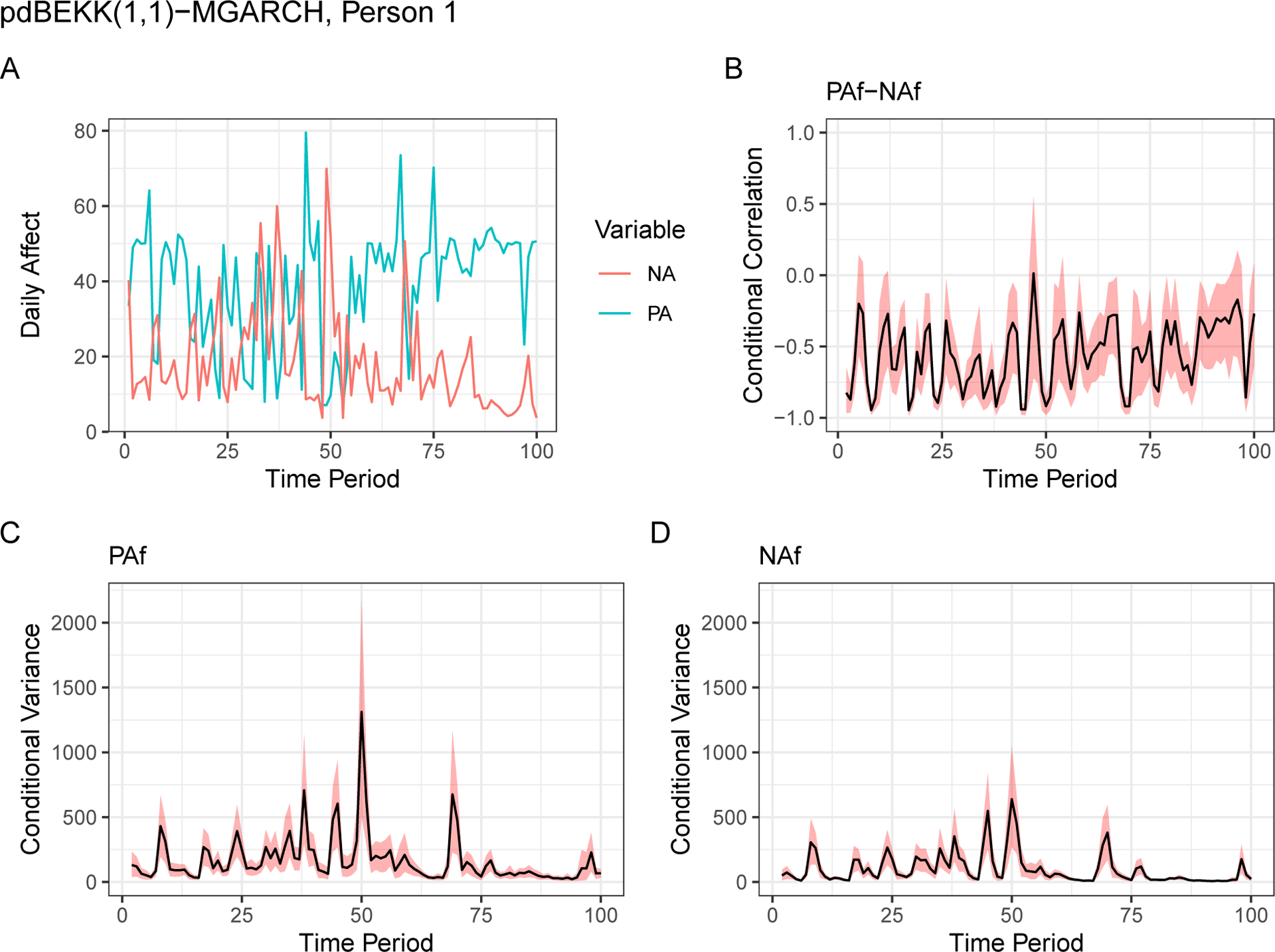
Observed data (panel A) and estimates for Individual 1 from the pdBEKK model. Panel B shows the estimated conditional correlation among PA and NA over the whole observation period of 100 days. Panels C and D show the corresponding conditional variances for the same period of time for PA and NA.

Figure 3.

Observed data (panel A) and estimates for Individual 6. Panel B shows the estimated conditional correlation among PA and NA over the whole observation period of 100 days. Panels C and D show the corresponding conditional variances for the same period of time for PA and NA.

Notably, while Individual 6 had a relatively large unconditional variance in NA compared to PA, the conditional variance shown in Panels C and D in Figure 3, suggests that PA was more variable over time. That is, while the baseline variance was smaller in PA, the effects of ARCH and GARCH ultimately resulted in a more variable conditional covariance in PA compared to NA.

The original, unscaled values (daily average of NA and PA) are shown in Panel A. The remaining effects for the means from the ARMA(1,1) model for both participants are reported in the Appendix in Table A1. The run time for this model was approximately four to five minutes on a Linux operated system with an IntelCore i7 at 3.4GHz, with 4 cores (8 threads) and 16 GiB RAM.

Discussion of pdBEKK results.

We picked two individuals that displayed a different pattern in terms of ARCH and GARCH parameters to illustrate the possibility of two different processes that drive the within-person variability. For one, both individuals showed no substantial “unconditional” correlations (R_PA,NA) probably also due to a lack of precision. This indicates that, in the baseline, the residuals of PA and NA were probably not correlated. Nonetheless, after including the effects of both ARCH and GARCH processes, the resulting conditional correlation R_t (derived from H_t) was overall strongly negative for Individual 1. This negative conditional correlation was mainly induced by the cross-over effects in the ARCH process, where previous day disturbances resulted in an opposite behavior with respect to NA and PA. That is, for Individual 1, random shocks tended to induce disparity among PA and NA responses in the sense that PA scores that fell above the expected value coincided with NA scores that fell below the expected value – and vice versa. This effect from the ARCH process implies that it will be pronounced after days when the random shock is large. This pattern was not found in the GARCH process for that same individual. In turn, Individual 6, showed a different pattern in terms of conditional correlations where only for a short period of time, approximately among day 10 to 35, the correlations tended to be negative. The source for these negative correlations in Individual 6, were in the GARCH process, which implies that this persons (co-)variances for NA always contain a fixed amount of the previous-day conditional variance of PA. That is, the negative spill-over effect in the GARCH process also results in a pattern where the PA variance from the previous day results in more disparate PA and NA responses for the current day. Both individuals tended to show larger carry over effects in the GARCH process but the size of the CrI also suggests that these parameters were less precisely estimated.

In order to modify the constant variance, we included the number of steps taken for each day as an external, but time-varying predictor. The inclusion of this variable served mainly as an example on how such a predictor could moderate the baseline variance. In this current application, daily steps did not seem to influence the conditional variance of neither PA nor NA.

Overall, these two individuals showed nuanced differences in the way their conditional variances came about. Also, it is important to note that they were selected to illustrate how BEKK can accommodate asymmetric variance spill overs from one time-series into the other and to highlight the two ARCH and GARCH processes.

DCC-MGARCH.

The time-series of PA and NA for the same two individuals were re-estimated with the DCC parameterization. Again, we included daily steps (on a z metric) as a predictor for the constant variance c and the mean response was modeled following an ARMA(1,1) model. The results for the DCC-MGARCH parameters are presented in Table 2 and the remaining results for the ARMA(1,1) parameters are reported in the Appendix in Table A2.

Table 2.

DCC(1,1)-MGARCH Estimates for Two Individuals

	Individual 1			Individual 6
	Estimate	CrI		Estimate	CrI
	Median	5%	95%	Median	5%	95%
β h0;PA	0.39	−1.3	1.85	0.54	−1.14	2.06
β h0;NA	0.98	−0.56	2.18	1.57	−0.59	2.97
β h1;PA	−0.42	−2.02	1.57	0.78	−1.34	1.92
β h1;NA	−0.52	−1.72	0.98	−0.06	−1.33	0.83
a hPA	0.13	0.06	0.26	0.22	0.07	0.56
a hNA	0.06	0.02	0.16	0.31	0.07	0.65
b hPA	0.73	0.56	0.84	0.68	0.41	0.88
b hNA	0.80	0.54	0.91	0.55	0.21	0.79
a q	0.09	0.01	0.28	0.19	0.07	0.33
b q	0.29	0.03	0.75	0.63	0.36	0.78
S q;NA	−0.68	−0.81	−0.47	−0.32	−0.70	0.14

Note. Posterior medians, 5% to 95% credible intervals (CrI) for two individuals. Parameters who’s posterior probability mass is above or below zero with p ≥ .95 are bolded. PA = Positive Affect, and NA = Negative Affect. S_q,NA represents the unconditional correlation among PA and NA throughout the full observation period. The a’s represent the ARCH parameters and the b’s represent the GARCH parameters. The subscript h is for the GARCH model for the standard deviations and the subscript q indicates parameters for the GARCH model in the conditional correlation. β₀ captures the intercept of the SD of PA and NA on the log scale encoded in the diagonal and β₁ is the regression weight of the predictor on the SD, so that diag(C) = exp(β₀ + β₁Steps)

The DCC has two submodels with ARCH and GARCH processes: One for the conditional standard deviations in D_t and the other for the dynamic conditional correlation R_t. The ARCH and GARCH parameters for PA and NA that operate on D_t are independent of each other, as such this model does not allow for asymmetric variance spill overs. The results for the DCC-MGARCH are reported in Table 2 where the parameters for the conditional variance are denoted by the subscript h and the parameters for the conditional correlation are denoted by the subscript q.

As with the BEKK model, the constant variance is given on the log scale in β_h0 and it represents the variance when the predictor (daily steps on z-scale) is at its average. For both individuals DCC estimated a non-zero constant variance (h_ii = exp(β₀)) for PA (median of Individual 1: h_PA = 1.48 with 90% CrI [0.27; 6.39]; median of Individual 6: h_PA = 1.71 with 90% CrI [0.32; 7.84]) and NA (median of Individual 1: h_NA = 2.67 with 90% CrI [0.57; 8.88]; median of Individual 6: h_NA = 4.81 with 90% CrI [0.55; 19.54]) while daily steps (β_h1) did not influence either of the constant variances.

The ARCH process, captured in the a_h parameters, as well as the GARCH process, captured in the b_h parameters, was positive for both individuals and the CrI’s indicate that more than 95% of the posterior mass was above 0. Generally, the GARCH process seemed to be larger than the ARCH process indicating that the conditional variance contains a larger portion of daily carry over effects compared to the absorption of previous day shocks (ARCH process).

In the second submodel, which operates on the conditional dynamic correlation R_t both individuals showed again non-zero ARCH and GARCH effects. The pattern was similar as in the first submodel in the sense that the dynamic correlation was affected more by autoregressive effects than by random shocks. Only Individual 1 showed a strong non-zero unconditional correlation S among PA and NA over the whole observation period.

The model implied conditional variances and correlations for both individuals are shown in Figures 4 and 5. The conditional correlation for Individual 1 remained relatively stable, and negative, over the observation period of 100 days. The conditional correlation for Individual 6 was generally comprising 0, except for the approximate period between day 10 and 35. The run time for this model was similar to the pdBEKK with approximately four to five minutes per individual.

Figure 4.

Observed data (panel A) and estimates for Individual 1 from the DCC model parameterization. Panel B shows the estimated conditional correlation among PA and NA over the whole observation period of 100 days. Panels C and D show the corresponding conditional variances for the same period of time for PA and NA.

Figure 5.

Observed data (panel A) and estimates for Individual 6. Panel B shows the estimated conditional correlation among PA and NA over the whole observation period of 100 days. Panels C and D show the corresponding conditional variances for the same period of time for PA and NA.

Discussion of DCC results.

The DCC parameterization does not allow for variance spill overs as it does not contain cross-lagged and asymmetric effects. Hence, all relations among the PA and NA variances need to be absorbed by the unconditional correlation S. As such, the DCC can be conceived as operating on two submodels, the conditional variances and the conditional dynamic correlation. While this separation eases the computational burden it somewhat complicates the interpretation as we have two layers that comprise ARCH and GARCH parameters. Interestingly, the unconditional correlation S for Individual 1 among PA and NA was strongly negative, which was also reflected in Panel B of Figure 4. Overall, all ARCH and GARCH parameters resulted in posteriors that largely excluded 0. As with the pdBEKK model, the constant variance term was larger for NA, especially for Individual 6 – but the resulting conditional variance was noticeably smaller for NA than PA (see Panel Dm Figure 5). This indicates that the conditional variance can drastically increase compared to its baseline variance, depending on how the ARCH and GARCH and its interrelation play out.

The predictor, daily steps, did not seem to have any measurable effect on the constant variance. Again, this predictor was mainly included as proof of concept to show how these types of parameters can be interpreted and included.

Comparison among BEKK and DCC.

Both models operate differently on the conditional variances and in order to have not only a visual comparison, such as in Figures 2 to 5, we compared the fit of both models via the predictive accuracy measures, PSIS-LOO and WAIC For both participants we computed the respective statistics to compare among the pdBEKK and the DCC parameterization (see Table 3). In both cases, the estimates were so close (within less that two SE’s of each other) that we were not able rank one model over the other in terms of fit. This is not too surprising, as BEKK and DCC have been shown to perform similarly well in simulation studies and empirical comparisons regarding forecasting conditions and in prediction of variance, covariances, and correlations (e.g. Caporin & McAleer, 2008; de Almeida et al., 2018; Huang, Su, & Li, 2010)

Table 3.

Comparison of pdBEKK- and DCC-MGARCH Models and Fit Statistics

	Model	PSIS-LOO (s.e.)	Δ PSIS-LOO (s.e)
Individual 1	pdBEKK	−227.1 (17.8)	–
Individual 1	DCC	−238.4 (18.2)	11.3 (6.3)
Individual 6	pdBEKK	−268.7 (13.1)	–
Individual 6	DCC	−272.9 (14.6)	4.2 (4.5)

Note. The difference in the PSIS-LOO (Δ PSIS-LOO) is with respect to the previous model reported in the row above for the same individual. The Δ PSIS-LOO does not suggest relevant differences among both model specifications, neither in Individual 1 nor in Individual 6.

Data Requirements.

The results of the pdBEKK and, to some degree the DCC model, yielded parameter estimates with very large CrI’s suggesting low precision and high uncertainty surrounding some of the MGARCH parameters. This was mainly observed for elements of the constant covariance matrix, in particular for the constant covariance in the pdBEKK model. A similarly high degree of uncertainty was observed for the corresponding univariate constant variance terms in the DCC model, whereas the constant correlation term S in DCC seemed to be estimated with higher precision. MGARCH models have been thoroughly investigated in simulation studies and real applications throughout the last two decades with the general consent that these models are robust in terms of prediction and forecasting (e.g Boussama, Fuchs, & Stelzer, 2011; Caporin & McAleer, 2014; Rossi & Spazzini, 2010). In the context of our work, however, it remains unclear what the data requirements are when these models are used on behavioral data. Most simulation studies concerned with evaluating the quality of the MGARCH parameter estimates are based on much longer time series than we used here. That is, while typically parameter bias is low and precision and recovery is high, all studies we are aware of, were based on at least 1,000 observations per time-series (e.g. Bauwens & Storti, 2013; Bauwens, Storti, & Violante, 2012; de Almeida et al., 2018). To shed some light on the data requirements when shorter time-series are used, we conducted a small scale post-hoc simulation for two times-series based on the values of Tables 1 and 2. For the simulation we drew 100 replications over five conditions comprising different time-series lengths of n ∈ {100, 200, 300, 500, 700} – the simulation took eight days to complete. In terms of statistical power, given the standard prior specifications in the bmgarch package, we mainly focused on the parameters that can contain zero in their 95% posterior probability mass. That is, for pdBEKK, the constant covariance (off-diagonal element of C) and the lagged cross-loadings in A and B were of interest. For DCC, only the constant correlation S_1,2 in S can comprise zero.

Table 1.

pdBEKK(1,1)-MGARCH Estimates for Two Individuals

	Individual 1			Individual 6
	Estimate	CrI		Estimate	CrI
	Median	5%	95%	Median	5%	95%
R PA,NA	0.09	−0.83	0.9	0.29	−0.9	0.95
β 0;PA	0.67	−1.14	1.7	0.18	−1.45	1.6
β 0;NA	0.32	−1.27	1.15	1.41	0.23	1.99
β 1;PA	−0.62	−1.45	0.88	0.14	−1.21	1.25
β 1;NA	−0.22	−1.16	1.1	−0.30	−1.41	0.13
A PA,PA	0.34	0.16	0.58	0.43	0.27	0.65
A PA,NA	−0.43	−0.64	−0.26	0.07	−0.08	0.19
A NA,PA	−0.35	−0.63	−0.1	0.03	−0.29	0.38
A NA,NA	0.16	0.03	0.36	0.53	0.13	0.86
B PA,PA	0.81	0.09	0.98	0.85	0.6	0.94
B PA,NA	−0.23	−0.47	0.36	−0.11	−0.27	−0.01
B NA,PA	0.63	−0.4	0.95	0.09	−0.35	0.62
B NA,NA	0.31	0.05	0.76	0.57	0.12	0.78

Note. Posterior medians, 5% to 95% credible intervals (CrI) for two individuals. Parameters who’s posterior probability mass is above or below zero with p ≥ .95 are bolded. PA = Positive Affect, and NA = Negative Affect. R_PA,NA represents the unconditional correlation among PA and NA throughout the full observation period. The A matrix contains the ARCH parameters and the B matrix the GARCH parameters. β₀ captures the intercept of the SD of PA and NA on the log scale encoded in the diagonal and β₁ is the regression weight of the predictor on the SD, so that diag(C) = exp(β₀ + β₁Steps)

For DCC, the lower value obtained from Individual 6 of S_1,2 = −.32 resulted in a frequentist power estimate π = .80 with a time series lengths of n = 100. pdBEKK, in turn, needed substantially more data to detect any of its parameters. Power for recovering the cross-lagged GARCH parameter B_1,2 of Individual 6 was π = .80 at a time-series length of approximately n = 600 and only about π = .20 with n = 200. The lagged cross-loadings in Individual 1’s ARCH process A generally required less data. The larger effect size of −.43 was sufficiently powered (π = .80) given a time-series length of 250 while the smaller effect of −.35 required approximately 400 datapoints to reach the same threshold. The constant covariance parameter C_1,2 was practically undetectable. Using the larger estimate (in correlation metric r = .29) from Individual 6 resulted in a power estimate of π = .50 in our condition with the longest time-series of 700. In terms of coverage, both DCC and pdBEKK, performed well – which is unsurprising as the model uncertainty mainly results in very wide CrI’s that will comprise the target values.

General Discussion

We set out to investigate MGARCH models for their use in psychological research. Originally, these models have been developed and are mainly used in the context of economic research on volatility forecasting and financial decision making. As such, the model itself is very well established and has been thoroughly tested and investigated. Over the course of two decades it has proven useful in a plethora of real life applications. To the best of our knowledge, however, it has not received much attention in psychology. The main attracting feature of these models is the partitioning of residual variance into different components that resemble ARMA processes for the means. Hence, the goal of this paper was to assess its usefulness in psychology, especially in research on within-person variability. Of all the model parameterizations, two prototypical approaches seemed best: the BEKK and the DCC Conceptually, BEKK models the conditional covariance directly, while DCC separates the conditional covariance into two elements: the conditional standard deviations of the univariate time-series and the conditional dynamic correlations. In terms of model fit and forecasting performance, both models (BEKK and DCC) fare similarly well, not only in our data but also in simulation and empirical applications discussed in the econometric literature. This finding is not surprising as these models have been used extensively over the last 20 years to model and forecast volatility in a plethora of conditions.

While the original BEKK parameterization was attractive, it can result in parameters that are difficult to understand. Hence, to facilitate the interpretation of the standard BEKK model, we included an additional constraint on the ARCH and GARCH parameter matrices to yield a model that is easier to interpret, the pdBEKK. Moreover, we added a custom parameterization for the constant variance and we provide an R-package (bmgarch) to estimate these models.

As noted, one of the differences among the pdBEKK and DCC parameterization is that the first models the conditional variance directly while the former operates on the separated elements. The approach of the DCC mainly reflects an effort to reduce computational burden as it is inherently easier to treat the conditional variances as univariate time-series and estimate the remaining correlations separately.

Hence, the distinction therefore must be drawn from an interpretability and from a feasibility perspective. The latter point refers to the “curse of dimensionality” (Bellman, 1961; Caporin & McAleer, 2012), of the BEKK which can only model a limited number of time-series. de Almeida et al. (2018), for example, were only able to estimate BEKK models with less than five simultaneous time-series while the DCC parameterization was able to accommodate up to 10. Our R-package bmgarch performed similarly; in a small simulation we were able to estimate up to seven time-series with the pdBEKK parameterization before all starting values were rejected and sampling was aborted. The DCC model did not run into these issues but the computation times increased drastically. While two time-series of length 200 converged within 1 minute, 10 time-series needed 12 minutes and 20 time-series 75 minutes.

As such, the decision on whether the DCC or BEKK parameterization is preferred also depends on the number of time-series one wishes to model. In that sense, DCC will be able to accommodate more simultaneous processes. However, while it might seem a limitation that we can only model up to five processes with BEKK, realistically, it becomes increasingly difficult to interpret all parameters in a sensible manner without simply scanning for non-zero effects and engage in post-hoc tale telling.

Overall, the BEKK seems to provide parameters that are both easier and richer in terms of interpretation. While the DCC returns two sets of ARCH and GARCH parameters, for the conditional standard deviations and the conditional correlation, it does not allow asymmetric variance spill-overs. This might be a limitation when capturing psychological processes. Moreover, while the ARCH and GARCH parameters are straightforward to interpreted on for the variances, their meaning is less evident for the conditional correlation. The BEKK, in turn estimates only one set of ARCH and GARCH parameters that directly model the conditional covariance. As such, its correspondence is more direct in terms of variances and covariances. Most importantly, the BEKK allows variance and covariance to be induced by the other variable and this lagged cross-over effect does not need to be symmetrical. This makes the BEKK interesting for investigations into within-person variability where one can imagine processes that induce variance in other processes.

As shown here, we can further include time-varying predictors for the conditional variance, illustrated with the number of steps taken daily to moderate the constant variance. While we did not find strong effects in the current application, it seems a necessary addition to account for external sources of variance. Note that Engle and Kroner (1995) introduced a model with an additional variance term, we decided to include a sub-model that can moderate the size of the constant variance, in order to also account for decreasing variances. Note that one could also expand the ARCH and GARCH processes to higher orders to investigate lag effects that exceed 1.

The limitations, in terms of usefulness of MGARCH models in psychological research, mostly come down to the complexity of the models and to the data requirements needed for a precise estimation. While statistical power will mostly pose no issue, for the parameters that only operate on one time-series (e.g. all diagonals in the pdBEKK, all parameters for D_t in DCC) as they are either constrained to be positive or tend to only produce positive values, it was evident form the results, that the correlation and cross-lagged effects are more difficult to estimate. Our small scale post-hoc simulation indicated that both models need lots of data in order to detect non-zero effects; which is especially pronounced for the pdBEKK parameterization. We would suggest that time-series lengths of 100 are generally too short to obtain stable estimates. This is not too surprising as previous research has shown (in population models) that long time series of within-person data are needed to obtain reliable estimates of intraidindividal variability (Estabrook, Grimm, & Bowles, 2012)

Moreover, MGARCH models in general are computationally burdensome and, as discussed, they are limited in the number of time-series that they can estimate simultaneously. Generally, the more moving parts, the fewer time-series can be estimated simultaneously and the more data is needed. As such, we see the use of these models mainly in the area of individualized modeling as MGARCH are inherently N=1 models. While one could exchange time-series variables for persons, we would only be able to investigate a few subjects at a time. This can be interesting, say for dyadic researchers but for the general population modeler, these GARCH models may be not be useful.

Importantly, given long enough time-series, both the pdBEKK and the DCC are able to partition the conditional covariances into sub-elements that can be interpreted in a psychologically relevant manner. While we prefer the pdBEKK in terms of interpretation and in terms of the ability to accommodate asymmetric variance spill-over, the DCC will be capable of estimating more simultaneous time-series and it seems to require less data.

Appendix

Table A1.

pdBEKK(1,1)-MGARCH ARMA(1,1) Estimates for Two Individuals

	Person 1			Person 6
	Estimate	CrI		Estimate	CrI
	Median	5%	95%	Median	5%	95%
ϕ 0;PA	41.41	35.16	47.6	44.04	38.23	49.71
ϕ 0;NA	23.09	15.83	30.24	28.92	24.69	32.43
ϕ PA	0.29	0.16	0.4	0.14	−0.08	0.33
ϕ PA,NA	−0.57	−0.78	−0.37	−0.40	−0.69	−0.06
ϕ NA,PA	−0.38	−0.51	−0.25	0.11	−0.03	0.3
ϕ NA	0.51	0.29	0.68	−0.14	−0.4	0.1
θ PA	−0.05	−0.23	0.15	0.32	0.07	0.55
θ NA	0.56	0.25	0.84	0.56	0.14	0.92
θ NA,PA	0.23	0.04	0.41	−0.21	−0.37	−0.06
θ NA	−0.33	−0.57	−0.03	0.25	0.03	0.49

Note. Posterior medians, 5% to 95% credible intervals (CrI) for three individuals. Parameters who’s posterior probability mass is above or below zero with p ≥ .95 are bolded. PA = Positive Affect, and NA = Negative Affect. ϕ₀ contains the intercept terms and ϕ the AR parameters. θ captures the MA process.

Table A2.

DCC(1,1)-MGARCH ARMA(1,1) Estimates for Two Individuals

	Individual 1			Individual 6
	Estimate	CrI		Estimate	CrI
	Median	5%	95%	Median	5%	95%
ϕ 0;PA	40.11	33.3	46.15	44.69	38.58	50.87
ϕ 0;NA	24.85	17.24	32.48	28.74	24.56	32.48
ϕ PA	0.20	0.02	0.35	0.14	−0.11	0.33
ϕ PA,NA	−0.17	−0.58	0.33	−0.44	−0.73	−0.05
ϕ NA,PA	−0.25	−0.39	−0.09	0.10	−0.03	0.27
ϕ NA	0.03	−0.46	0.43	−0.13	−0.37	0.09
θ PA	0.07	−0.18	0.31	0.32	0.09	0.56
θ PA,NA	0.06	−0.5	0.63	0.63	0.14	0.95
θ NA,PA	0.07	−0.17	0.31	−0.20	−0.36	−0.06
θ NA	0.20	−0.29	0.73	0.20	−0.03	0.44

Note. Posterior medians, 5% to 95% credible intervals (CrI) for three individuals. Parameters who’s posterior probability mass is above or below zero with p ≥ .95 are bolded. PA = Positive Affect, and NA = Negative Affect. ϕ₀ contains the intercept terms and ϕ the AR parameters. θ captures the MA process.

References

- Akaike H (1973). Information Theory and an Extension of the Maximum Likelihood Principle. In Petrov BN & Csaki F (Eds.), Second international symposium on information theory (pp. 267–281). [Google Scholar]
- Almeida DM, Piazza JR, & Stawski RS (2009). Interindividual differences and intraindividual variability in the cortisol awakening response: An examination of age and gender. Psychology and Aging, 24 (4), 819–827. Retrieved from http://doi.apa.org/getdoi.cfm?doi=10.1037/a0017910 doi: 10.1037/a0017910 [DOI] [PMC free article] [PubMed] [Google Scholar]
- Bauwens L, & Laurent S (2005). A New Class of Multivariate Skew Densities, With Application to Generalized Autoregressive Conditional Heteroscedasticity Models. Journal of Business & Economic Statistics, 23 (3), 346–354. Retrieved from http://www.tandfonline.com/doi/abs/10.1198/073500104000000523 doi: 10.1198/073500104000000523 [DOI] [Google Scholar]
- Bauwens L, Laurent S, & Rombouts JVK (2006). Multivariate GARCH models: a survey. Journal of Applied Econometrics, 21 (1), 79–109. Retrieved from http://doi.wiley.com/10.1002/jae.842 doi: 10.1002/jae.842 [DOI] [Google Scholar]
- Bauwens L, & Storti G (2013). Computationally Efficient Inference Procedures for Vast Dimensional Realized Covariance Models. In Grigoletto M & Petrone S (Eds.), Complex models and computational methods in statistics (pp. 37–49). Milano: Springer. doi: 10.1007/978-88-470-2871-5_4 [DOI] [Google Scholar]
- Bauwens L, Storti G, & Violante F (2012). Dynamic conditional correlation models.pdf.
- Bellman R (1961). Adaptive control processes: A guided tour. Princeton, NJ: Princeton University Press. [Google Scholar]
- Bollerslev T (1986). Generalized autoregressive conditional heteroskedasticity. Journal of Econometrics, 31 (3), 307–327. Retrieved from http://linkinghub.elsevier.com/retrieve/pii/0304407686900631 doi: 10.1016/0304-4076(86)90063-1 [DOI] [Google Scholar]
- Bollerslev T (1990, aug). Modelling the Coherence in Short-Run Nominal Exchange Rates: A Multivariate Generalized Arch Model. The Review of Economics and Statistics, 72 (3), 498. Retrieved from https://www.jstor.org/stable/2109358?origin=crossref doi: 10.2307/2109358 [DOI] [Google Scholar]
- Bollerslev T, Engle RF, & Wooldridge JM (1988). A Capital Asset Pricing Model with Time-Varying Covariances. Journal of Political Economy, 96 (1), 116–131. Retrieved from http://doi.wiley.com/10.3982/ECTA9240 doi: 10.1086/261527 [DOI] [Google Scholar]
- Boussama F, Fuchs F, & Stelzer R (2011). Stationarity and geometric ergodicity of BEKK multivariate GARCH models. Stochastic Processes and their Applications. doi: 10.1016/j.spa.2011.06.001 [DOI] [Google Scholar]
- Bringmann LF, Lemmens LHJM, Huibers MJH, Borsboom D, & Tuerlinckx F (2015). Revealing the dynamic network structure of the Beck Depression Inventory-II. Psychological Medicine, 45 (4), 747–757. Retrieved from https://www.cambridge.org/core/product/identifier/S0033291714001809/type/journal{_}article doi: 10.1017/S0033291714001809 [DOI] [PubMed] [Google Scholar]
- Bürkner P-C, Gabry J, & Vehtari A (2019, feb). Approximate leave-future-out cross-validation for Bayesian time series models. Retrieved from http://arxiv.org/abs/1902.06281
- Caporin M, & McAleer M (2008). Scalar BEKK and indirect DCC. Journal of Forecasting, 27 (6), 537–549. Retrieved from http://doi.wiley.com/10.1002/for.1074 doi: 10.1002/for.1074 [DOI] [Google Scholar]
- Caporin M, & McAleer M (2012). Do we really need both BEKK and DCC? A tale of two multivariate GARCH models. Journal of Economic Surveys, 26 (4), 736–751. Retrieved from http://doi.wiley.com/10.1111/j.1467-6419.2011.00683.x doi: 10.1111/j.1467-6419.2011.00683.x [DOI] [Google Scholar]
- Caporin M, & McAleer M (2014, aug). Robust ranking of multivariate GARCH models by problem dimension. Computational Statistics & Data Analysis, 76, 172–185. Retrieved from https://linkinghub.elsevier.com/retrieve/pii/S0167947312002113 doi: 10.1016/j.csda.2012.05.012 [DOI] [Google Scholar]
- Carnero MA, & Eratalay MH (2014). Estimating VAR-MGARCH models in multiple steps. Studies in Nonlinear Dynamics & Econometrics, 18 (3), 339–365. Retrieved from https://www.degruyter.com/view/j/snde.2014.18.issue-3/snde-2012-0065/snde-2012-0065.xml doi: 10.1515/snde-2012-0065 [DOI] [Google Scholar]
- Castro-Schilo L, & Ferrer E (2013). Comparison of Nomothetic Versus Idiographic-Oriented Methods for Making Predictions About Distal Outcomes From Time Series Data. Multivariate Behavioral Research, 48 (2), 175–207. Retrieved from http://www.tandfonline.com/doi/abs/10.1080/00273171.2012.736042 doi: 10.1080/00273171.2012.736042 [DOI] [PubMed] [Google Scholar]
- Cleveland WS, Denby L, & Liu C (2002). Random scale effects (Tech. Rep.). Murray Hill, NJ: Statistics Research Dept. Bell Labs. Retrieved from https://citeseerx.ist.psu.edu/viewdoc/download?doi=10.1.1.141.2403{&}rep=rep1{&}type=pdf [Google Scholar]
- de Almeida D, Hotta LK, & Ruiz E (2018). MGARCH models: Trade-off between feasibility and flexibility. International Journal of Forecasting, 34 (1), 45–63. Retrieved from https://www.sciencedirect.com/science/article/pii/S0169207017300894 doi: 10.1016/J.IJFORECAST.2017.08.003 [DOI] [Google Scholar]
- Engle RF (1982). Autoregressive Conditional Heteroscedasticity with Estimates of the Variance of United Kingdom Inflation. Econometrica, 50 (4), 987. Retrieved from https://www.jstor.org/stable/1912773?origin=crossref doi: 10.2307/1912773 [DOI] [Google Scholar]
- Engle RF (2002). Dynamic Conditional Correlation. Journal of Business & Economic Statistics, 20 (3), 339–350. Retrieved from http://www.tandfonline.com/doi/abs/10.1198/073500102288618487 doi: 10.1198/073500102288618487 [DOI] [Google Scholar]
- Engle RF, & Kroner KF (1995). Multivariate simultaneous generalized arch. Econometric Theory, 11 (1), 122–150. Retrieved from http://www.journals.cambridge.org/abstract{_}S0266466600009063 doi: 10.1017/S0266466600009063 [DOI] [Google Scholar]
- Engle RF, & Sheppard K (2001). Theoretical and Empirical properties of Dynamic Conditional Correlation Multivariate GARCH (Tech. Rep.). Cambridge, MA: National Bureau of Economic Research. Retrieved from http://www.nber.org/papers/w8554.pdf doi: 10.3386/w8554 [DOI] [Google Scholar]
- Epskamp S, van Borkulo CD, van der Veen DC, Servaas MN, Isvoranu A-M, Riese H, & Cramer AOJ (2018). Personalized Network Modeling in Psychopathology: The Importance of Contemporaneous and Temporal Connections. Clinical Psychological Science, 6 (3), 416–427. Retrieved from http://journals.sagepub.com/doi/10.1177/2167702617744325 doi: 10.1177/2167702617744325 [DOI] [PMC free article] [PubMed] [Google Scholar]
- Estabrook R, Grimm KJ, & Bowles RP (2012, sep). A Monte Carlo simulation study of the reliability of intraindividual variability. Psychology and Aging, 27 (3), 560–576. Retrieved from http://ezproxy.library.uvic.ca/login?url=http://search.ebscohost.com/login.aspx?direct=true{&}db=pdh{&}AN=2012-02078-001{&}site=ehost-live{&}scope=sitehttp://content.ebscohost.com/ContentServer.asp?T=P{&}P=AN{&}K=2012-02078-001{&}S=L{&}D=pdh{&}EbscoContent=dGJyMNXb4kSep7Y doi: 10.1037/a0026669 [DOI] [PMC free article] [PubMed] [Google Scholar]
- Ferrer E, Gonzales JE, & Steele J (2013). Intra- and Interindividual Variability of Daily Affect in Adult Couples. GeroPsych: The Journal of Gerontopsychology and Geriatric Psychiatry, 26 (3), 163–172. doi: 10.1024/1662-9647/a000095 [DOI] [Google Scholar]
- Fisher AJ, Reeves JW, Lawyer G, Medaglia JD, & Rubel JA (2017). Exploring the idiographic dynamics of mood and anxiety via network analysis. Journal of Abnormal Psychology, 126 (8), 1044–1056. Retrieved from http://doi.apa.org/getdoi.cfm?doi=10.1037/abn0000311 doi: 10.1037/abn0000311 [DOI] [PubMed] [Google Scholar]
- Fiske DW, & Rice L (1955). Intra-individual response variability. Psychological Bulletin, 52 (3), 217–250. Retrieved from http://doi.apa.org/getdoi.cfm?doi=10.1037/h0045276 doi: 10.1037/h0045276 [DOI] [PubMed] [Google Scholar]
- Gelman A, & Carlin J (2014). Beyond Power Calculations. Perspectives on Psychological Science, 9 (6), 641–651. Retrieved from http://journals.sagepub.com/doi/10.1177/1745691614551642 doi: 10.1177/1745691614551642 [DOI] [PubMed] [Google Scholar]
- Gelman A, & Rubin DB (1992, nov). Inference from Iterative Simulation Using Multiple Sequences. Statistical Science, 7 (4), 457–472. Retrieved from http://projecteuclid.org/euclid.ss/1177011136 doi: 10.1214/ss/1177011136 [DOI] [Google Scholar]
- Geweke J (1993, dec). Bayesian treatment of the independent student-t linear model. Journal of Applied Econometrics, 8 (S1), S19–S40. Retrieved from http://doi.wiley.com/10.1002/jae.3950080504 doi: 10.1002/jae.3950080504 [DOI] [Google Scholar]
- Hamaker EL, Asparouhov T, Brose A, Schmiedek F, & Muthén B (2018). At the Frontiers of Modeling Intensive Longitudinal Data: Dynamic Structural Equation Models for the Affective Measurements from the COGITO Study. Multivariate Behavioral Research, 53 (6), 820–841. Retrieved from https://www.tandfonline.com/doi/full/10.1080/00273171.2018.1446819 doi: 10.1080/00273171.2018.1446819 [DOI] [PubMed] [Google Scholar]
- Hedeker D, & Mermelstein RJ (2007). Mixed effects regression models with heterogeneous variance: Analyzing ecological momentary assessment (EMA) data of smoking. In Little TD, Bovaird JA, & Card NA (Eds.), (pp. 183–206). Mahwah, NJ.: Lawrence Erlbaum. [Google Scholar]
- Hedeker D, Mermelstein RJ, & Demirtas H (2008). An Application of a Mixed-Effects Location Scale Model for Analysis of Ecological Momentary Assessment (EMA) Data. Biometrics, 64 (2), 627–634. Retrieved from http://doi.wiley.com/10.1111/j.1541-0420.2007.00924.x doi: 10.1111/j.1541-0420.2007.00924.x [DOI] [PMC free article] [PubMed] [Google Scholar]
- Huang Y, Su W, & Li X (2010). Comparison of BEKK GARCH and DCC GARCH Models: An Empirical Study. In Lecture notes in computer science (Vol. 6441 LNAI, pp. 99–110). Retrieved from http://link.springer.com/10.1007/978-3-642-17313-4{_}10 doi: 10.1007/978-3-642-17313-4_10 [DOI] [Google Scholar]
- Leckie G, French R, Charlton C, & Browne W (2014). Modeling Heterogeneous Variance-Covariance Components in Two-Level Models. Journal of Educational and Behavioral Statistics, 39 (5), 307–332. Retrieved from http://journals.sagepub.com/doi/10.3102/1076998614546494 doi: 10.3102/1076998614546494 [DOI] [Google Scholar]
- Lewandowski D, Kurowicka D, & Joe H (2009). Generating random correlation matrices based on vines and extended onion method. Journal of Multivariate Analysis, 100 (9), 1989–2001. doi: 10.1016/j.jmva.2009.04.008 [DOI] [Google Scholar]
- Lindley DV (1971). The estimation of many parameters. In Godambe VP & Sprott DA (Eds.), (pp. 435–455). Toronto: Holt, Rinehart, and Winston. [Google Scholar]
- Molenaar PCM, Huizenga HM, & Nesselroade JR (2003). The relationship between the structure of interindividual and intraindividual variability: A theoretical and empirical vindication of developmental systems theory. In Staudinger UM & Lindenberger U (Eds.), (pp. 339–360). Dordrecht, Netherlands: Kluwer Academic Publishers. Retrieved from http://link.springer.com/chapter/10.1007/978-1-4615-0357-6{_}15 [Google Scholar]
- Molenaar PCM, Sinclair KO, Rovine MJ, Ram N, & Corneal SE (2009). Analyzing developmental processes on an individual level using nonstationary time series modeling. Developmental psychology, 45 (1), 260–71. Retrieved from http://www.ncbi.nlm.nih.gov/pubmed/19210007 doi: 10.1037/a0014170 [DOI] [PubMed] [Google Scholar]
- Natesan P, & Hedges LV (2017). Bayesian unknown change-point models to investigate immediacy in single case designs. Psychological Methods, 22 (4), 743–759. Retrieved from http://doi.apa.org/getdoi.cfm?doi=10.1037/met0000134 doi: 10.1037/met0000134 [DOI] [PubMed] [Google Scholar]
- Nesselroade JR, & Molenaar PCM (2010). Emphasizing Intraindividual Variability in the Study of Development Over the Life Span Concepts and Issues. In Lerner RM, Lamb ME, & Freund AM (Eds.), The handbook of life-span development (pp. 30–54). Hoboken, NJ, USA: John Wiley & Sons, Inc. doi: 10.1002/9780470880166 [DOI] [Google Scholar]
- O’Laughlin KD, Liu S, & Ferrer E (2020). Use of Composites in Analysis of Individual Time Series: Implications for Person-Specific Dynamic Parameters. Multivariate Behavioral Research, 1–18. Retrieved from https://www.tandfonline.com/doi/full/10.1080/00273171.2020.1716673 doi: 10.1080/00273171.2020.1716673 [DOI] [PubMed] [Google Scholar]
- Ram N, & Gerstorf D (2009). Time-structured and net intraindividual variability: Tools for examining the development of dynamic characteristics and processes. Psychology and Aging, 24 (4), 778–791. Retrieved from http://doi.apa.org/getdoi.cfm?doi=10.1037/a0017915 doi: 10.1037/a0017915 [DOI] [PMC free article] [PubMed] [Google Scholar]
- Rast P, & Ferrer E (2018). A Mixed-Effects Location Scale Model for Dyadic Interactions. Multivariate Behavioral Research, 53 (5), 756–775. Retrieved from https://www.tandfonline.com/doi/full/10.1080/00273171.2018.1477577 doi: 10.1080/00273171.2018.1477577 [DOI] [PMC free article] [PubMed] [Google Scholar]
- Rast P, Hofer SS, & Sparks C (2012). Modeling Individual Differences in Within-Person Variation of Negative and Positive Affect in a Mixed Effects Location Scale Model Using BUGS/JAGS. Multivariate Behavioral Research, 47 (2), 177–200. doi: 10.1080/00273171.2012.658328 [DOI] [PubMed] [Google Scholar]
- Rindskopf D (2014). Nonlinear Bayesian analysis for single case designs. Journal of School Psychology, 52 (2), 179–189. Retrieved from https://linkinghub.elsevier.com/retrieve/pii/S0022440513001143 doi: 10.1016/j.jsp.2013.12.003 [DOI] [PubMed] [Google Scholar]
- Rossi E, & Spazzini F (2010). Model and distribution uncertainty in multivariate GARCH estimation: A Monte Carlo analysis. Computational Statistics & Data Analysis, 54 (11), 2786–2800. Retrieved from https://linkinghub.elsevier.com/retrieve/pii/S0167947309002345 doi: 10.1016/j.csda.2009.06.004 [DOI] [Google Scholar]
- Rush J, Rast P, Almeida DM, & Hofer SM (2019). Modeling long-term changes in daily within-person associations: An application of multilevel SEM. Psychology and Aging, 34 (2), 163–176. Retrieved from http://doi.apa.org/getdoi.cfm?doi=10.1037/pag0000331 doi: 10.1037/pag0000331 [DOI] [PMC free article] [PubMed] [Google Scholar]
- Shadish WR (2014). Statistical Analyses of Single-Case Designs: The Shape of Things to Come. Current Directions in Psychological Science, 23 (2), 139–146. Retrieved from http://journals.sagepub.com/doi/10.1177/0963721414524773 doi: 10.1177/0963721414524773 [DOI] [Google Scholar]
- Shadish WR, Rindskopf DM, Hedges LV, & Sullivan KJ (2013). Bayesian estimates of autocorrelations in single-case designs. Behavior Research Methods. doi: 10.3758/s13428-012-0282-1 [DOI] [PubMed] [Google Scholar]
- Stan Development Team. (2016). The Stan C++ Library (2.14.0 ed.). Retrieved from http://mc-stan.org
- Sullivan KJ, Shadish WR, & Steiner PM (2015). An introduction to modeling longitudinal data with generalized additive models: Applications to single-case designs. Psychological Methods. doi: 10.1037/met0000020 [DOI] [PubMed] [Google Scholar]
- Tsay RS (2013). An Introduction to Analysis of Financial Data with R.
- van der Krieke L, Emerencia AC, Bos EH, Rosmalen JG, Riese H, Aiello M, … de Jonge P (2015). Ecological Momentary Assessments and Automated Time Series Analysis to Promote Tailored Health Care: A Proof-of-Principle Study. JMIR Research Protocols, 4 (3), e100. doi: 10.2196/resprot.4000 [DOI] [PMC free article] [PubMed] [Google Scholar]
- Vehtari A, Gelman A, & Gabry J (2017). Practical Bayesian model evaluation using leave-one-out cross-validation and WAIC. Statistics and Computing, 27, 1413–1432. doi: 10.1007/s11222-016-9696-4 [DOI] [Google Scholar]
- Vehtari A, & Ojanen J (2012). A survey of Bayesian predictive methods for model assessment, selection and comparison. Statistics Surveys, 6, 142–228. Retrieved from http://projecteuclid.org/euclid.ssu/1356628931 doi: 10.1214/12-SS102 [DOI] [Google Scholar]
- Watanabe S (2010). Asymptotic Equivalence of Bayes Cross Validation and Widely Applicable Information Criterion in Singular Learning Theory. Journal of Machine Learning Research, 11, 3571–3594. Retrieved from http://jmlr.csail.mit.edu/papers/volume11/watanabe10a/watanabe10a.pdf [Google Scholar]
- Watson D (1988). Intraindividual and interindividual analyses of positive and negative affect: Their relation to health complaints, perceived stress, and daily activities. Journal of Personality and Social Psychology, 54, 1020–1030. [DOI] [PubMed] [Google Scholar]
- Wei WW (2013). Time Series Analysis. In The oxford handbook of quantitative methods in psychology: Vol. 2: Statistical analysis (pp. 458–485). Oxford: Oxford University Press. doi: 10.1093/oxfordhb/9780199934898.013.0022 [DOI] [Google Scholar]
- Williams DR, Mulder J, Rouder J, & Rast P (2020). Beneath the Surface: Unearthing Within-Person Variability and Mean Relations with Bayesian Mixed Models. Psychological Methods, 1–24. Retrieved from https://psyarxiv.com/gwatq/ doi: 10.31234/OSF.IO/GWATQ [DOI] [PMC free article] [PubMed] [Google Scholar]
- Woodrow H (1932). Quotidian variability. Psychological Review, 39 (3), 245–256. doi: 10.1037/h0073076 [DOI] [Google Scholar]