Perspective: Planning and Conducting Statistical Analyses for Human Nutrition Randomized Controlled Trials: Ensuring Data Quality and Integrity

Abstract

Appropriate planning, execution, and reporting of statistical methods and results is critical for research transparency, validity, and reproducibility. This paper provides an overview of best practices for developing a statistical analysis plan a priori, conducting statistical analyses, and reporting statistical methods and results for human nutrition randomized controlled trials (RCTs). Readers are referred to the other NURISH (NUtrition inteRventIon reSearcH) publications for detailed information about the preparation and conduct of human nutrition RCTs. Collectively, the NURISH series outlines best practices for conducting human nutrition research.

Statement of Significance: This paper provides an overview of best practices for developing a statistical analysis plan a priori, conducting statistical analyses, and reporting statistical methods and results for human nutrition, randomized, controlled trials.

Introduction

At the foundation of good clinical nutrition research practice is a comprehensive and detailed plan that defines the study design (described by Lichtenstein et al. (1)), documentation and regulatory procedures (described by Weaver et al. (2)), laboratory processes and data collection management (described by Maki et al. (3)), as well as the statistical analyses to be conducted (discussed herein). In addition, reporting complete, clear, and transparent results from human nutrition randomized controlled trials (RCTs) is critical for knowledge transfer, critical appraisal, and development of evidence-based guidance. These papers originated from the NURISH (NUtrition inteRventIon reSearcH) Project, a workshop that was held to discuss best practices for the conduct of human nutrition research (4).

According to the American Statistical Association, statistical practice emphasizes principles of good study design and conduct, and interpretation followed by reporting of results in context (5). Therefore, the statistical analysis phase of a human nutrition RCT should not be viewed as a distinct component that is done independently of the other phases. Rather, consideration of the statistical methods should underpin all aspects of an RCT, including development of the specific aims and design of the protocol, execution of the trial, data management and analyses, and interpretation and reporting of the findings.

To ensure adequate consideration of the statistical methods for human nutrition RCTs, best practice is to develop an a priori statistical analysis plan. The results and interpretation of the findings should be presented in alignment with the pre-defined statistical approach. The aim of this paper is to describe the development of a statistical analysis plan including timing, key components, and presentation of results.

Statistical analysis plan and execution

A statistical analysis plan should be prepared at the time of protocol development and finalized prior to database lock and unblinding of randomization codes (Figure 1). The statistical analysis plan may be posted to a platform such as Open Science Network (https://osf.io) where the registration date is time-stamped for enhanced transparency. Prior to database lock and unblinding of randomization codes, the statistical analysis plan should be updated to reflect any changes to the design, conduct, or proposed statistical analyses that may have occurred because of several factors including funding availability, trial implementation issues, or the availability of new evidence from trials reporting out since the commencement of the project. The importance of this cannot be overstated because proper inference requires full reporting and transparency. For valid conclusions to be drawn from a publication reporting results from an RCT, the number of hypotheses tested, key data collection decisions, statistical analyses conducted, and resulting statistical summaries for primary and secondary outcomes should be reported. Care should be taken to optimize the design and minimize the risk of type I (false positives) and type II (false negatives) statistical errors.

FIGURE 1.

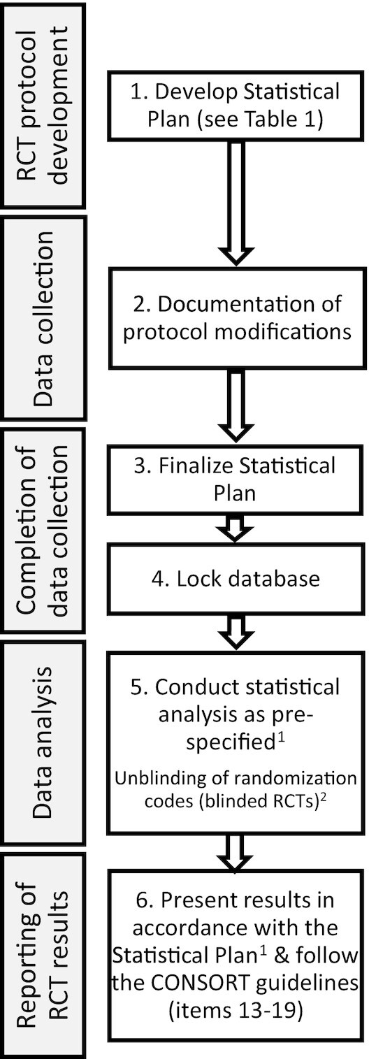
How the statistical analysis plan fits into the overall conduct and reporting of human nutrition RCTs. ¹Statistical analyses not pre-defined should be treated as exploratory and clearly identified as such in the reporting of results. ²Unblinding of randomization codes for RCTs with blinded allocation should occur following the database lock as part of the data analysis phase. RCT, randomized controlled trial.

Table 1 outlines elements that should be included in a human nutrition RCT statistical analysis plan. Many of these components are common to the statistical analysis plan requirements for NIH grants and therefore the statistical analysis plan may be formulated as part of a grant application. If the statistical analysis plan is not written as part of a grant application, it may be written as part of the protocol development phase of the RCT or may be developed as a separate document containing more details than are provided in the protocol (Figure 1). In the subsequent sections, detailed information about what should be included in each section of a human nutrition RCT statistical analysis plan is summarized including best practices for using and implementing the statistical analysis plan throughout the entire life of a human nutrition RCT.

TABLE 1.

Items that should be addressed in a statistical analysis plan for a human nutrition RCT¹

Section and Item
Section 1: Administrative information
Title and clinical trial registration number
Analysis plan version, including revisions
Roles and responsibilities of key personnel
Section 2: Introduction
Background and rationale for the trial
Study objectives
Section 3: Study methods
Trial design
Randomization/allocation concealment/blinding procedures
Sample size justification/calculations
Framework for hypothesis testing (e.g., superiority, non-inferiority,equivalence)
Planned interim analyses and stopping rules, if applicable
Timing of outcome assessments and analysis
Section 4: Trial population
Screening data and eligibility criteria
Recruitment
Early withdrawal of participants
Presentation of baseline characteristics
Section 5: Analysis population(s)
Analysis populations (e.g., intention-to-treat, per protocol, completers,safety)
Adherence/compliance and protocol deviations/violations
Section 6: Hypothesis testing
Multiple hypothesis tests (multiplicity)
Number of groups or conditions
Number of outcome variables evaluated
Composite outcome variables
Section 7: Statistical analysis
Outcome variable definitions
Accounting for covariates
Repeated measurements
Missing data
Additional planned analyses (e.g., sensitivity, subgroup, exploratoryanalyses)
Safety and tolerability analyses
Data presentation
Statistical software

¹RCT, randomized controlled trial.

Section 1. Administrative information

The administrative information for a trial is in the first section of the statistical analysis plan. It includes the protocol title and clinical trial registration number, as well as the statistical analysis plan number and protocol version number, including amendments, if applicable. This section should also cover the roles and responsibilities of key personnel, including the Principal Investigator and Co-investigator(s), biostatistician(s), data manager, and others (e.g., project manager, clinician monitor, medical monitor), depending on the size of the trial. The sponsor and location(s) of the study may also be included.

Section 2. Introduction

The introduction section of a statistical analysis plan summarizes the background and rationale for the study as well as the study objectives. This information is often taken directly from the grant proposal and/or study protocol.

Section 3. Study methods

The study methods should be described in the statistical analysis plan, with particular attention to the following components that will inform the statistical approaches for the RCT.

Trial design

The study design should be described, including the comparisons to be tested, the duration of the study, and the timing of data collection. Other design aspects that should be described include the run-in period and/or washout period(s).

Randomization method, allocation concealment, blinding

Randomization is a critical step that balances characteristics between allocation units. Allocation units may be at the individual participant level or group level (e.g., household, clinic, community), depending on the study design and aims. It is imperative that the randomization schedule cannot be anticipated, that is, the treatment or treatment sequence allocation is concealed from study personnel until assignment (described by Lichtenstein et al. (1)). The method used to generate the randomization schedule should be detailed in the statistical analysis plan, including the use of stratification, if applicable. A stratified randomization schedule can be used to ensure that 1 or more characteristics of the study sample that are expected to be strongly related to the outcome are approximately equally distributed across groups. However, if stratification is used, the number of stratification variables should be limited to a small number of factors that are expected to be strongly associated with the response or outcome, most often 1 or 2 (6). For example, in the Reduction of Cardiovascular Events with Icosapent Ethyl-Intervention Trial (REDUCE-IT) (7), a trial to assess the impact of 4 g/d of icosapent ethyl (ethyl esters of eicosapentaenoic acid) vs. placebo on major adverse cardiovascular events, randomization was stratified according to cardiovascular risk (secondary prevention or primary prevention; with primary prevention capped at 30% of enrolled patients), ezetimibe use, and geographic region. In some instances, stratification is used to ensure adequate representation of subgroups that are expected to be difficult to recruit, or for which subgroup analyses are planned. For example, sex stratification will ensure that there is not a large imbalance in the male to female ratio across groups, even if the study sample is 80% female and 20% male (i.e., ∼4:1 in all study groups/conditions). In other cases, a stratified randomization scheme will be used to ensure that randomization is balanced by a particular characteristic, for example, 50% in a lower stratum (150–199 mg/dL) for baseline triglyceride concentration and 50% in a higher stratum (200–499 mg/dL). Once a randomization stratum is filled, only individuals that meet the criteria for the stratum or strata with available slots are randomized. Therefore, when using stratified randomization, the feasibility of recruiting for and filling each randomization stratum/strata should be considered. If a stratified randomization schedule is used, the stratification categories should be included as factors in the statistical models used to assess the intervention effects.

The statistical analysis plan should also detail how allocation concealment was achieved. Allocation concealment occurs when personnel involved in the enrollment of participants to the study have no knowledge of the allocation sequence prior to a participant's randomization. A lack of foreknowledge of the randomization assignment avoids the potential for conscious or subconscious influence on the randomization sequence, such as directing a person with a more severe condition to the active intervention rather than the control. The randomization process will result in groups that are approximately equivalent with regard to known and unknown confounding factors; a lack of allocation concealment may inadvertently alter this balance. To conceal allocation, the randomization schedule should be developed by a member of the research team who is not involved in the screening or enrollment of participants into the study. At the time of participant allocation, randomization should be done using opaque, sealed, and sequentially pre-numbered envelopes (conventional methodology), a computer program that is accessed through the internet (interactive web response system, e.g., REDCap) or a telephone system (interactive voice response system). These methods should be detailed in the statistical analysis plan as well as the timing of randomization.

Blinding, or being naïve to the intervention allocation, mitigates ascertainment bias (or detection bias) by masking the allocation sequence for the duration of the study among participants, outcome assessors, and the statistician(s) who will analyze study data. Blinding study personnel who assess outcomes will limit bias in the collection and interpretation of data; for example, judgment about whether an adverse experience is likely to be attributable to the intervention. Participant blinding reduces the risk of randomization knowledge affecting the outcomes rather than the treatment or condition. Participant blinding in human nutrition RCTs is often not feasible because many research questions do not enable concealment (see Lictenstein et al. (1) for more detail). In some circumstances, it is advisable to ensure that participants do not come into contact with one another to avoid unblinding. For example, if there is a side effect of the study intervention (e.g., flushing with niacin supplementation), discussions between subjects might lead individual participants to conclude that they have been assigned to the active or placebo condition. The methods used to ensure that the pre-specified randomization schedule is followed, and blinding is maintained, if applicable, should be described in the statistical analysis plan.

Sample size estimate on assumptions for primary outcome

The target sample size for a trial is typically estimated based on assumptions for the primary outcome(s) (i.e., variable(s) to be measured). A power analysis is conducted to determine the number of subjects needed to detect an intervention's effect at a pre-specified alpha (typically 0.05, 2-sided) and power (typically 80% or 90%) levels. Power for secondary aims may be lower or higher if the sample size is determined based on the primary outcome. For key secondary outcomes, a separate sample size calculation may be warranted, which may result in recruitment of a larger number of participants to ensure sufficient power for both primary and key secondary outcomes. An expected loss to follow-up rate may be added to the recruitment goal to ensure the target sample size is achieved. The sample size estimate reported in the statistical analysis plan should include all of the assumptions and parameters entered into the power calculation (e.g., test, alpha, sidedness, variance, effect size) with appropriate justification to support the feasibility of the estimate. In some cases, no data may be available for the estimated effect size and variance because of the novelty of the research question, which should be stated and other methods of determining the sample size outlined (e.g., convenience sample, available resources). Sample size calculations have been described in more detail by Lichtenstein et al. (1).

Framework for hypothesis testing

In human nutrition RCTs the objective is typically to compare one or more experimental condition(s) (i.e., the intervention group or condition) with one or more control group(s) or condition(s) for an outcome of interest. The outcome can be a continuous variable such as LDL-cholesterol concentration or a categorical variable such as new-onset type 2 diabetes mellitus.

Standard practice is to state hypotheses as a null (no difference between conditions) and an alternative (there is a difference between conditions) since statistical tests are based on rejecting the null hypothesis or failing to reject the null. In most cases, the alternative hypothesis will be non-directional (i.e., there is a difference being the default), although it can be stated as a directional hypothesis (e.g., vitamin D supplementation to correct deficiency will lower the incidence of fractures more than the placebo). If there are more than 2 groups or conditions, hypotheses are typically tested in a stepwise manner. The first (omnibus) hypothesis is that there are no differences among the conditions and, if the first hypothesis is rejected, additional hypotheses are tested between individual conditions (i.e., post hoc, pairwise tests). A different approach is to a priori define contrasts as described in Section 6.

P-values and alpha level for hypothesis testing:A P-value is an assessment of the probability of a result equal to or more extreme than the observed result under the assumption that the null hypothesis is correct and is used to assess the extent of the evidence against the null hypothesis. If the P-value is sufficiently small, we reject the null hypothesis; otherwise, we conclude that the data do not provide sufficient evidence to reject the null hypothesis. The alpha level is the P-value that is used as a cut-off for rejection of the null hypothesis, and has traditionally been 0.05, 2-sided, when a single hypothesis is being tested. In Section 6, additional considerations for the alpha level used are described.

P-values should not be viewed or reported as strictly dichotomous indicators. Absolute P-values should be reported, where possible, rather than P-value cut points (e.g., P < 0.05). It is not true that a P-value of 0.04 indicates that the effect of an intervention is physiologically and clinically important, while a P-value of 0.06 indicates that the effect is physiologically and clinically unimportant. A small, clinically unimportant effect can produce a P-value less than 0.05 if the sample size is large and/or the measurement precision is very high. Conversely, a large, clinically important effect may result in a P-value above 0.05 if the sample size is small or measurements are imprecise (8, 9). This is one reason why sample size determination using a clearly rationalized power calculation is so important.

With a 2-sided alpha of 0.05, there is a 5% probability of a false positive, that is, rejecting a null hypothesis that is true. A false positive is also known as a type I statistical error. When the null hypothesis is false (i.e., the alternative is true) and a statistical test fails to reject it, this is a type II statistical error. A common reason for a type II statistical error is a sample size that is too small, resulting in insufficient statistical power. Type I and type II statistical errors are covered in more detail by Lichtenstein et al. (1). It should be noted that some methodologists believe that a 5% risk of a false positive result is insufficiently rigorous and leads to acceptance of efficacy for interventions that lack clinically important benefits too often. Therefore, some have proposed adoption of a more stringent threshold for declaring statistical significance such as 1% (P = 0.01) or 0.5% (P = 0.005) (9, 10).

Testing for difference, equivalence, or non-inferiority:The usual hypothesis test applied in human nutrition RCTs is for a difference between or among intervention groups/conditions, which is equivalent to testing the null hypothesis that the conditions are not different, with the alternative hypothesis that they are not all the same. This can be expressed as follows for the null hypothesis (H₀) and alternative hypothesis (H_a) in a study with 2 groups (or conditions for a crossover study), A and B.

• H₀: mean for group A = mean for group B

• H_a: mean for group A ≠ mean for group B

In some instances, the hypothesis being tested is one of equivalence. For example, this approach can be used to test for bioequivalence, based on the maximum concentration (C_max) and the AUC, for 2 drug formulations, such as a reference version and a version seeking approval as a generic substitute for the reference agent (i.e., the comparator). These procedures can also be used for evaluating bioavailability and bioequivalence for nutrients in dietary supplements. The standard used by the FDA to demonstrate bioequivalence in drug studies is a geometric mean ratio and 90% CI that fall within the range of 0.80 to 1.25 (11). A geometric mean ratio (antilog of the mean of the logs) is used because logarithmic transformation of pharmacokinetic data is recommended (12). These principles can also be applied to dietary supplements (13, 14). For other applications, a different range may be used (15).

The following profile would support an inference of bioequivalence, using the FDA criteria (11), of 2 products (i.e., a drug or a dietary supplement) because both the C_max and AUC geometric mean ratios show 90% CIs that do not extend beyond the boundaries of 0.80 and 1.25:

• Comparator geometric mean C_max/reference geometric mean C_max = 1.06 (90% CI: 0.88, 1.22)

• Comparator geometric mean AUC/reference geometric mean AUC = 1.03 (90% CI: 0.86, 1.19)

In some trials the hypothesis being tested is non-inferiority, that is, the comparator intervention is equivalent or superior to the reference intervention. For example, a weight loss trial designed to assess whether an intervention administered via online instruction (i.e., the comparator) is non-inferior to a reference intervention administered via in-person group meetings (i.e., the reference). The test for non-inferiority is based on a maximum margin by which the comparator could underperform without being considered clinically inferior. If the upper bound of the 90% or 95% CI (depending on the alpha selected) excludes this margin, non-inferiority would be supported, otherwise the alternative hypothesis (inferiority) would be supported. In this example, a non-inferiority margin of 3% is used with a 95% CI. If mean weight loss is 8.2% in the reference group and 6.6% in the online intervention group, the mean difference between the groups would be 1.6%. Whether or not the non-inferiority hypothesis is supported would depend on whether the 95% CI for the mean difference crosses the 3% non-inferiority margin. For example:

• Mean difference (95% CI): 1.6% (0.9, 2.3%), non-inferiority hypothesis supported

• Mean difference (95% CI): 1.6% (0.1, 3.1%), non-inferiority hypothesis not supported

Interim analyses

Some RCTs incorporate one or more a priori planned interim analyses into the trial design for the purpose of decision-making about whether to continue the trial or to stop the trial because of benefit or harm of the intervention, or very low likelihood of demonstrating benefit if completed (i.e., futility analyses). For example, the Look AHEAD (Action for Health in Diabetes) trial was stopped after 9.6 years because of a recommendation from the data and safety monitoring board based on a futility analysis showing low probability (i.e., 1%) of observing a significant positive result at the planned end of follow-up (i.e., a HR of 0.82 in the intervention group) (16). Short-term studies do not tend to have interim analyses for trial termination, but interim analyses might be used to verify the assumptions used in the original sample size and power calculations. If the assumptions do not appear to have been accurate, the trial can be resized, based on observed data, to ensure the study has adequate statistical power.

To account for the completion of multiple statistical tests in the final analysis (i.e., for the interim plus final analyses), procedures must be in place for “alpha spending” or distributing the type I error rate across the planned analyses. Some alpha is used for the interim analysis(es) and the remaining alpha is then applied to the final analysis. The degree of alpha spending used for the interim analysis(es) depends on the alpha used to declare statistical significance in the interim analysis(es), and the fraction of the information from the overall trial available at the time of the interim analysis(es) (17).

Timing of outcome assessments and analysis

Outcome measurement timing should be pre-specified for both primary and secondary outcomes. This should include outcome definitions, methods used to assess outcomes, time points of outcome measurement (time frame for visit windows), and frequency of follow-up. In some instances, follow-up may continue after the primary outcome has been assessed. For example, the primary outcome in a weight loss trial may be weight loss after 1 year, but follow-up may continue for a second year. In such cases, analysis of first year data may proceed while participants are still being followed during the second year.

Section 4. Trial population

 

Screening data and eligibility criteria

The participant inclusion and exclusion criteria should be specified in the study protocol and summarized in the statistical analysis plan (see Lichtenstein et al. (1) for details about defining inclusion/exclusion criteria). Inclusion criteria should clearly specify the population included in terms of age range, sex, anthropometric data, health status (presence or absence of specific diseases), medication and dietary supplement use, biochemical values, and lifestyle habits. Exclusion criteria should state the populations that are being excluded. The eligibility criteria should provide a clear rationale for the target population, including justification for exclusion of certain population subgroups (e.g., if the study is limited to English-speaking participants), since this can affect the generalizability of the results. The timing of the data collection and processing of this information to evaluate eligibility should be described. Procedures for possible modification of the criteria to meet recruitment goals or other unforeseen issues should be specified. Any changes to the study protocol over time should be carefully documented so that such changes can be considered when the data are analyzed, and the results are interpreted.

Recruitment

Methods used for recruitment should be described in the statistical plan as this may have implications for the representativeness of the sample (see Lichtenstein et al. (1) for more details about recruitment methods).

Early withdrawal of participants (participant dependent, investigator dependent)

A participant enrolled in a study may decide to withdraw from the trial completely, or only from specific procedures at any time, or may opt to discontinue participation for a period of time and then rejoin the trial. If a subject opts out of specific procedures, follow-up data collection may continue for some of the study measures that the participant agrees to continue. The investigator may also withdraw participants from the trial for a variety of reasons, including non-adherence, development of a condition that would potentially confound the interpretation of the study results for that participant, or that might increase the risks to the participant should they continue. The statistical analysis plan must address the handling of missing data because of early termination and other reasons. Guidance on the handling of missing data in statistical analyses has been provided by the National Research Council's Committee on National Statistics (18, 19).

Presentation of baseline characteristics

Item 15 of CONSORT Statements provide recommendations for baseline data reporting (20, 21). For example, for randomized parallel group trials a table showing baseline demographic and clinical characteristics for each group should be presented (20). For randomized crossover studies, a table showing baseline demographic and clinical characteristics by sequence and period should be presented (21). Descriptive statistics (see Section 7) should be presented for baseline characteristics. Baseline characteristics should be presented for the pre-specified main analysis population and potentially secondary analysis populations (see Section 5). Statistical testing for baseline differences between randomization groups/sequences is not recommended because any differences that exist occur because of chance and therefore statistical testing is redundant (20). Instead, the clinical and prognostic significance of any differences in central tendency or distribution of baseline characteristics between groups/conditions should be evaluated using clinical judgment.

Section 5. Analysis population(s)

 

Analysis populations

Analysis populations should be defined in the statistical analysis plan and all decisions regarding the analysis populations should be made prior to database lock and unblinding of the randomization codes for a blinded trial. It should be noted that the term “analysis population” is in common usage, although it can be argued that the term analysis samples would be more appropriate, since a sample is a group selected from a population by a defined procedure. In a clinical trial, a sample is recruited from a larger population and enrolled into the trial based on pre-defined entry criteria.

The FDA defines analysis populations as the set of subjects whose data are to be included in the main analyses and secondary analyses. The choice of analysis population should be aligned with the objective(s) of the RCT; however, minimizing bias and avoiding inflation of the risk of type I statistical errors should also inform the decisions made. Other considerations include whether the aim is to examine effectiveness (conducted under conditions mimicking “real-world” implementation) or efficacy (conducted under ideal conditions), if self-reported or objective measures of adherence will be collected, and the sample size.

Typically, an intention-to-treat analysis is conducted, that is, an analysis based on the initial, random allocation, even if the participant withdraws from the study, did not comply, or received a different intervention. An intention-to-treat analysis must often contend with missing data, such as data for participants who discontinued participation in the study or who missed some of the scheduled assessments. Analyses consistent with intention-to-treat principles may have missing data, although assumptions about the randomness of the missing data will inform appropriate handling of this issue, which is beyond the scope of this paper. The interested reader is referred to the following references prepared by the National Research Council's Committee on National Statistics (18, 19). Additional analysis populations may be included, such as a per-protocol analysis, which is limited to only participants who completed the trial with a pre-specified minimum level of adherence to the study intervention and no major protocol deviations or violations, which may be appropriate for efficacy trials. A safety population, which is used to assess the safety of the treatment/intervention, including adverse events, toxicity, and any clinical/biochemical effects, is often defined as all participants randomized who consumed at least 1 dose or serving of the study product. The statistical analysis plan should specify how data are to be analyzed for participants with poor intervention adherence (e.g., include in the intention-to-treat analysis, but exclude from the per-protocol analysis).

Adherence and protocol deviations/violations

The statistical analysis plan must include how adherence and protocol deviations/violations will be defined for the purpose of data analysis if a per-protocol analysis will be conducted. Methods for assessing adherence that may be used to define per-protocol analyses are detailed by Lichtenstein et al. (1).

Section 6: Hypothesis testing

Plans for hypothesis testing need to be described in the study protocol because the number of hypothesis(es) to be tested impacts the type I error rate and appropriate considerations (described later) are needed for managing this risk.

Multiple hypothesis tests (multiplicity)

Human nutrition RCTs with more than 2 interventions or more than 1 outcome variable need to address the issue of multiplicity, the appropriate control of statistical errors when drawing conclusions using more than 1 significance test. When particular versions of the alternative hypothesis are of interest, contrasts can be used to examine them (22). Each of these must be formulated as part of the statistical analysis plan. Since the alternative hypotheses represent separate research questions, each is tested using a critical P-value of 0.05. For example, consider a human nutrition RCT with 3 interventions: a control and 2 interventions that are very similar. The questions of interest could, for example, be formulated as 2 contrasts: the first comparing the control with the average of the 2 active interventions and the second comparing the 2 active interventions. If alternative hypotheses are not formulated a priori, then the multiplicity issue must be addressed in terms of a general alternative that typically includes a comparison of all pairs of interventions for each of the outcome variables. The general approach is to adjust the P-value needed to declare statistical significance.

As the number of hypothesis tests from a single RCT increases, so does the risk of type I statistical errors (false positives). If 100 statistical hypothesis tests are completed, each with an alpha of 0.05, for which the null hypothesis is true, we expect that approximately 5 false positive test results would occur with P ≤ 0.05. Therefore, as the number of tests increases, the alpha level used for each test should be adjusted downward to maintain the overall risk of a type I error at 0.05. Note that the multiplicity issue also applies to CIs. Accordingly, use of a lower alpha to account for multiple comparisons is often accompanied by adjusted CIs.

There are 3 key multiplicity considerations:

• Number of groups or conditions to be compared,

• Number of outcome variables evaluated, and

• Whether any interim analyses have been undertaken (see Interim Analyses section).

Number of groups or conditions

The number of comparisons increases rapidly as the number of intervention groups/conditions increases. With 2 interventions, there is a single simple comparison, the difference between the 2 interventions. With 3 interventions, there are 3 possible simple comparisons; with 4 interventions, the number of simple comparisons is 6, and with 5 interventions, there are 10 possible simple comparisons. It should also be noted that if additional analyses are conducted to assess between- or within-group/condition change from baseline this will also inflate the risk of type I statistical error (23, 24). Commonly, when the primary analysis is a comparison of endpoint means between groups/conditions, additional analyses are conducted to assess the change from baseline for outcomes between groups/conditions (i.e., between-group change from baseline analysis) or changes from baseline separately in each group/condition (i.e., within-group change from baseline analysis). Within-group/condition comparisons to baseline are generally not recommended because these are reflective of a time effect (23, 24) and an essential feature of RCTs is analyses that are focused on between-group/condition comparisons.

The typical approach for managing the risk of false positive hypothesis tests is to use an omnibus (also known as a global) test such as the F-ratio for ANOVA first, followed by pairwise comparisons only if the null hypothesis for the omnibus test is rejected at the specified alpha level (typically 0.05). For example, in a parallel-arm study with 4 intervention conditions, the ANOVA F-ratio would test the hypothesis that all group means are equal:

• H₀: mean 1 = mean 2 = mean 3 = mean 4

• H_a: at least 1 pair of means is not equal

If the F-ratio from the ANOVA has a P < 0.05, then pairwise testing can proceed. Various procedures are available for pairwise (also known as post hoc) testing. These methods adjust the alpha level to account for the number of pairwise tests being conducted to maintain the overall (familywise) risk of a false positive at 5% or less. The simplest method for adjusting the alpha is the Bonferroni correction, which simply divides the overall alpha by the number of comparisons to be undertaken as the threshold for declaring statistical significance. For example, in a study with 4 intervention conditions, there are 6 possible simple comparisons between allocation means:

1. 1 vs. 2

2. 1 vs. 3

3. 1 vs. 4

4. 2 vs. 3

5. 2 vs. 4

6. 3 vs. 4

In this example, the Bonferroni corrected alpha would be 0.05/6 = 0.0083. Thus, significance would be declared only if a pairwise test produced a P-value of <0.0083. The Bonferroni method is highly conservative, which results in a heightened risk of a type II statistical error compared with other types of procedures. Alternatives include the Tukey-Kramer and simulation-based procedures, which are appropriate when simple comparisons (i.e., pairwise comparisons) are being undertaken. In some instances, it is of primary interest to compare a single group (e.g., a control group) to each of the other groups. Dunnett's test may be used for this purpose, which would result in 3 pairwise comparisons for the above example, with 3 active intervention groups and a control group.

More sophisticated methods that conserve statistical power, compared with traditional approaches, include the Holm-Bonferroni (25) and Benjamini-Hochberg procedures (26). Full descriptions of these and other pairwise testing methods are beyond the scope of this paper. The overarching principle is that simply applying pairwise comparison tests, such as multiple t-tests, across groups results in an inflated risk of type I statistical errors (false positives). Therefore, investigators should apply appropriate procedures to protect the familywise error rate when more than 2 groups or conditions are being compared. These methods limit the number of tests being completed by using hierarchical testing procedures and/or by adjusting the alpha used to declare statistical significance to account for the number of statistical hypothesis tests completed.

Number of outcome variables evaluated

The statistical analysis plan for a human nutrition RCT should pre-specify all primary and secondary outcome variables and how these will be tested, including the alpha level that will be applied to each test, or how that alpha level will be determined. Outcome variable features should be specified, including time point(s), form (e.g., endpoint means, change from baseline, % change from baseline), and analysis population (e.g., intention-to-treat, completers, per protocol). The statistical model should also be pre-specified, including whether covariate adjustment will be employed and, if so, how the specific covariates will be determined (e.g., pre-specified or determined through an objective decision tree). Objective decision trees are created before data analysis begins and explicitly describe how data analyses will be conducted with objective criteria that dictate analysis decisions rather than using a results-driven approach that inflates the type I statistical error risk.

If an RCT has a single primary outcome variable and only 2 conditions/groups, a 2-sided alpha of 0.05 is generally used. If there are 2 co-primary outcome variables, the issue of multiple testing can be handled in several ways. One is to adjust the alpha level used for each test, such as with a Bonferroni correction, with half of the alpha allocated to each test (0.05/2 = 0.025). Other methods such as the Holm-Bonferroni (25) and Benjamini-Hochberg (26) procedures could be utilized, which will often result in higher statistical power than the more conservative Bonferroni method. Another approach is to specify a hierarchy in which one pre-specified variable is tested first, followed by continued testing only if the first null hypothesis is rejected. A detailed discussion of methods to protect the familywise type I error rate is beyond the scope of this paper. Interested readers are referred to 2 FDA guidance documents for more information (27, 28).

For trials with a factorial design, where subjects are randomly assigned to a treatment, then to 1 or more additional treatments, the analysis plan should specify the methods that will be used to account for potential interactions between treatments. For example, in the VITAL (Vitamin D and Omega-3) Trial (29), subjects were randomly assigned to receive vitamin D or placebo and also omega-3 fatty acids or placebo, resulting in 4 categories: vitamin D placebo + omega-3 placebo, vitamin D + omega-3 placebo, vitamin D placebo + omega-3, and vitamin D + omega-3. If a statistically significant or clinically relevant interaction is present for effects of treatments, the methods used for analysis will have to account for such interactions, which will have implications for the statistical power to test main effects.

Many human nutrition RCTs assess several secondary outcome variables. The clinical relevance of changes in 1 variable may require an understanding of how the intervention affects other outcomes. For example, a human nutrition RCT may examine the effect of an intervention on serum LDL-cholesterol as the primary outcome (variable). However, if the intervention lowers LDL-cholesterol while worsening other cardiometabolic risk factors such as systolic blood pressure or serum triglyceride concentration, one could not unequivocally conclude that the intervention produced a net benefit on the risk factor profile. In settings like this, it is necessary to assess multiple outcome variables.

For many human nutrition RCTs, secondary and exploratory outcome variables are tested at a 2-sided alpha of 0.05, without adjustment of the alpha to account for the number of comparisons. These secondary and exploratory variables can be highly correlated with the primary outcome variable, for example in an RCT where change in systolic blood pressure is the primary outcome variable, and change in diastolic blood pressure is a secondary outcome variable. Interpretation of the results of secondary and exploratory outcomes should be made with caution and acknowledge the risk for type I statistical error. For example, if 1 primary and 5 secondary outcome variables are tested, the risk of a type I error using an alpha of 0.05 for each test is 1—0.95⁶ = 0.265 or 26.5%. However, using a Bonferroni correction for each test would mean that an alpha of 0.05/6 = 0.0083 would be required to designate statistical significance. Few human nutrition RCTs are large enough to meet this level of rigor in statistical testing. Therefore, it is recommended that investigators report exact P-values for secondary outcomes and state clearly that there is an elevated risk of type I statistical error in secondary and exploratory outcome analyses. This is also true for sensitivity analyses such as those done in secondary analysis populations (e.g., completer or per protocol, when the intention-to-treat analysis is primary). It is also recommended that the primary outcome is the focus of nutrition RCT abstracts and if secondary and/or exploratory outcomes are reported in the abstract, these should be clearly identified as such. Furthermore, reporting of sensitivity and subgroup analyses in the abstract should usually be avoided, with the exception of statements indicating that the results were consistent across several subgroup and sensitivity analyses.

An important element of study design is to specify in advance a hierarchy of outcome variables in order to protect against an inflated risk of false positive findings. Generally, this involves pre-specification of a single primary outcome variable, or a small number of co-primary outcome variables, as well as a group of secondary outcome variables. Additional variables may be identified as exploratory. Moreover, additional variables may be assessed statistically (e.g., body weight change during the intervention) to assess potential confounding. Finally, statistical tests may be run for the purpose of assessing safety and tolerability of the intervention. It is therefore not uncommon for the analysis of results for a human nutrition RCT to include statistical tests on many variables.

The emergence of “omics” methods that generate a large amount of data, termed “big data” presents multiplicity challenges and specialized statistical methods are needed to control for the false discovery rate in these very large complex datasets. A bioinformatician or statistician should be consulted for these types of datasets. The interested reader is referred to the following methodological papers that outline key principles for “big data” analysis (30–35).

Composite outcome variables

In clinical event trials a composite outcome is often used, whereby the occurrence of several clinical events equally contributes towards the primary endpoint. For example, PREDIMED (Prevención con Dieta Mediterránea) (36) had a primary cardiovascular event endpoint that was a composite of myocardial infarction, stroke, or death from cardiovascular causes. Individual components and related events such as revascularization procedures can be included as secondary outcome variables. In some instances, a hierarchical testing procedure may be employed to minimize the risk of false positives where testing proceeds in a pre-specified order and stops when a test fails to produce a P-value <0.05. An example of a study that used a hierarchical testing procedure is REDUCE-IT (7). VITAL (29) is an example of how trial findings may be interpreted when the results from pre-specified secondary outcomes confirm hypotheses, but the primary outcome does not confirm the main trial hypothesis (Box 1).

Box 1:

Interpretation of results from pre-specified secondary outcomes when the primary outcome does not confirm the main trial hypothesis

In recent years it has become more common for journal editors to insist on de-emphasizing results from pre-specified secondary outcomes if the primary outcome shows no significant difference between treatment conditions. Results for secondary outcomes that suggest benefits for an intervention when the primary outcome shows no statistically significant difference are often interpreted as hypothesis generating (37). For example, in the omega-3 fatty acid arm of the Vitamin D and Omega-3 Trial (VITAL) that assessed supplementation of individuals at average cardiovascular risk with 1 g/d of omega-3 acid ethyl esters containing ∼840 mg/d of eicosapentaenoic acid and docosahexaenoic acid, there was no significant difference between the placebo and omega-3 intervention groups for the primary composite outcome of major cardiovascular events (HR 0.92; 95% CI: 0.80, 1.06) (29). However, there were reductions in some cardiac-related events, such as total myocardial infarction (HR 0.72; 95% CI: 0.59, 0.90) and total coronary heart disease (HR 0.83; 95% CI: 0.71, 0.97).

As suggested by Pocock and Stone (37) in some instances, results for secondary outcomes may be compelling enough to affect clinical and public health guidelines. Such secondary findings must be interpreted cautiously to ensure that there is a low probability of false positives, such as a P-value small enough to remain statistically significant after adjustment for the number of comparisons made using a conservative approach such as a Bonferroni correction. It is essential for investigators to clearly pre-specify a hierarchy of variables prior to unblinding to aid interpretation of findings. This may include specification of primary, key secondary, secondary, and exploratory analyses. Such a hierarchy will typically be based on what is known from prior investigations and the physiological effects of the intervention under study. Creating this hierarchy will be very helpful for limiting the number of statistical comparisons for which adjustment must be applied (i.e., alpha spending) and interpreting the findings. Findings for key secondary and secondary outcomes suggestive of benefit that align with results from previous investigations will be given more weight in the interpretation of findings than pre-specified exploratory outcomes, and especially those from any post hoc exploratory analyses.

In the case of VITAL (29), the results for cardiac-related secondary outcomes did not show unequivocal evidence of benefit after consideration of the number of statistical comparisons. However, the results were consistent with those from prior studies, which had shown mixed results, but generally supported a potential benefit of supplementation with lower dosages of omega-3 fatty acids (≤1.8 g/d) for some cardiac outcomes, particularly coronary heart disease death, but no benefit for stroke (38). Subsequent to the publication of results from VITAL, a meta-analysis of data from 119,244 subjects (including 25,871 VITAL participants) in 12 large-scale trials of lower-dosage omega-3 fatty acid interventions, compared with placebo or usual care, showed pooled estimates for myocardial infarction (RR 0.92; 95% CI: 0.86, 0.99, P = 0.02) and coronary heart disease death (RR 0.92; 95% CI: 0.86, 0.98, P = 0.014) consistent with modest, but statistically significant, benefits of supplementation (39). No benefit was observed for incidence of stroke in pooled analyses (RR 1.05; 95% CI: 0.98, 1.14, P = 0.183).

Pocock and Stone (37) use the example of a trial (Anglo-Scandinavian Cardiac Outcomes Trial) comparing 2 antihypertensive agents for which the primary outcome of non-fatal myocardial infarction plus fatal coronary heart disease showed no significant difference (P = 0.11), but secondary outcomes such as fatal and non-fatal stroke, and death from cardiovascular causes (i.e., those related to cardiac and stroke events), did show strong statistical significance, with P-values ≤0.001 and 95% CIs that were not close to the null value. Given strong statistical evidence of benefit for these secondary outcomes with the comparator agent (amlodipine), and that prior research had shown that antihypertensive treatments typically have larger effects on stroke outcomes than cardiac outcomes, the results for these secondary outcomes were considered compelling enough on their own to support recommendations to avoid using the reference agent (atenolol) as first-line therapy for hypertension (37).

Section 7. Statistical analysis

The statistical analysis section in the statistical analysis plan should describe the analysis methods and how the intervention effects will be presented. It is important to specify both the outcomes and endpoints that will be used in statistical analyses. An outcome is defined as the measured variable (e.g., LDL-cholesterol) whereas an endpoint is the analyzed variable (e.g., change from baseline at 6 weeks in LDL-cholesterol). The statistical analysis plan should distinguish between analyses designed to understand and interpret results, such as diagnostic plots to examine statistical model assumptions, versus analyses designed to explain the results to others, such as plots to effectively communicate the research findings. In addition to analyses designed to address specific aims and primary outcomes, additional analyses supporting ideas for future research can be included, such as subgroup and exploratory analyses.

Preliminary issues related to the statistical analyses that need to be addressed in the statistical plan include:

• Clear definitions, including analysis form, for all measured variables;

• Specification of procedures for identification and management of outliers with a description of how such outlying values will be handled in the analysis;

• Plans for checking model or statistical test assumptions;

• Methods for dealing with missing and incomplete data.

The statistical methods used will be determined by the variable type being examined, whether covariates and confounders need to be accounted for, and whether the dataset contains repeated measures. Statistical methods that are routinely used in clinical nutrition studies will not be discussed here; the interested reader can refer to statistics texts (40, 41). Rather, we focus on several principles that should inform the statistical plan and data analysis procedures.

Outcome variable definitions

The appropriate statistical methods for analysis will vary according to outcome variable type (level), which are categorized as scale (continuous), nominal (categorical with no intrinsic ordering), or ordinal (categorical with intrinsic ordering) for data analysis purposes. Many commonly used methods for statistical inference are based on an assumption that sample means, regression coefficients, or other statistical summaries follow a distribution that is approximately normal. Non-parametric methods, including simulation-based procedures, provide alternative approaches that do not involve the assumption of approximate normality.

Accounting for covariates

Randomized controlled parallel trials should ideally be designed in a manner that controls for variables with a high potential to influence the response to the intervention (i.e., confounders) to reduce the need for covariate adjustment. Stratification in the randomization schedule may be used to ensure balance across groups for such variables. When stratification is used for this purpose, the stratification factor must be included in the statistical models used for hypothesis testing.

Pre-randomization variables, commonly referred to as covariates, known in advance to be strongly associated with an outcome can be included in the statistical model. These can be quantitative variables or categorical variables measured prior to the commencement of the intervention. Variables measured after the start of the active/reference intervention should not be included as covariates because they are considered a response to the intervention allocation and interact dynamically with the outcomes (42). A quantitative variable may be discretized, although there is a potential trade-off between the loss of information versus the facilitation of the interpretation of results. For example, in the Glucosamine/chondroitin Arthritis Intervention Trial (GAIT) (43) the primary outcome was a 20% decrease in knee pain from baseline to week 24, which represents a discretization of the scale knee pain variable. For a given endpoint, the baseline value is often a strong predictor of response and therefore is frequently included as a pre-specified covariate. Such variables should be described in the statistical analysis plan with a rationale provided for inclusion, and the number should be limited to a few that are known to be related to the outcome(s), such as baseline value, sex, and possibly age. It should be noted that in the 2010 CONSORT Statement for parallel group randomized trials it is recommended that if covariate adjustment is conducted then both adjusted and unadjusted analyses should be presented (20).

Inclusion of covariates in an analysis has 2 potential effects. First, the residual variation in a model can be reduced, thereby increasing the power of the significance testing procedures used. In the simplest form, the residual variation is the mean squared error used as the denominator in an F-test; a smaller denominator means that the ratio is larger. Second, estimates of the outcomes can change if there are large differences in the means of the covariate across randomization groups. In this situation, we say that the outcome is adjusted for or controlled for the covariate. The adjusted means are what we would estimate the means to be if the groups had equal means for the covariate. Consideration of this issue should be carefully examined when the study is designed and the analysis plan is formulated. The statistical cost of including these variables, factors, or covariates, is minimal, involving a transfer of a few degrees of freedom from an error term to a model term in most linear models. An extreme case can occur when there is an attempt to make groups similar by matching on a collection of variables. With one-to-one matching, for example, a substantial loss of error degrees of freedom is consumed by adding terms to the model that account for the matching.

Baseline imbalances between groups for factors other than the dependent variable that were not expected but were observed post hoc should not be included as covariates in the primary analysis (44). However, the influence of baseline differences that are deemed to be clinically or prognostically significant may be evaluated in sensitivity and exploratory analyses to assess the robustness of the primary statistical analysis.

Repeated measurements

Outcome variables that are measured at multiple time points can be incorporated in statistical analysis in different ways. In some cases, a repeated measures ANOVA or mixed-model analysis are appropriate choices. Alternatively, the end-of-intervention value may be used as the outcome of interest with intermediate values assessed as secondary or exploratory analyses. In some specific circumstances, a summary of the repeated measures such as the slope of the change in values over time may be used as the outcome (e.g., carotid intima media thickness (45) or renal function (46–48)), although this approach can be challenging due to missing data. The approach to be employed should be pre-specified in the analysis plan.

A randomized crossover design is often referred to as a repeated measures design. In this design, more than 1 measurement is taken on each participant, and participants serve as their own comparison. Thus, it is important to distinguish the participant-to-participant (between-participant) variation and the within-participant variation in the model. One way to view this characteristic is through the correlation between measures on the same participant. In crossover trials the potential for order or carryover effects also needs to be assessed. Similarly, for a multi-site study, the correlation between measures at the same site should be modeled, although for studies with many sites, geographical region may be used in place of site. Clustered sampling, such as sampling participants within households, can be modeled in the same way. Mixed models allow modeling of both random and fixed effects (factors), which is appropriate for situations with repeated measurements. Random effects are factors that are expected to differ across participants (e.g., subject), whereas fixed effects are factors that are assumed to have the same effect across participants (e.g., diet, age, sex, race, ethnicity).

Missing data

Missing data are unavailable values that were planned to be collected. In human nutrition RCTs data may be missing for many reasons including, but not limited to, non-adherence to the study intervention, despite willingness to continue with follow-up for outcome assessment, or early withdrawal from the study because the participant is no longer available for the study including outcome assessment (49). Missing data affect a key assumption of randomization, known and unknown characteristics are balanced between allocation units, and thus the approach for managing missingness must be clearly delineated in the analysis plan with consideration for the assumptions underlying different methods. Details about methods for handling missing data are beyond the scope of this paper; methods for dealing with missing data in nutrition RCTs have been published previously (50). The interested reader is referred to a National Research Council report on the prevention and treatment of missing data in clinical trials (19).

Additional planned analyses

Sensitivity analyses: Sensitivity analyses are conducted to determine the robustness of a finding by examining how the result is affected by changes in methods, models, values of unmeasured variables, or assumptions (51). If the findings of the primary analyses align with the sensitivity analyses this increases confidence in the results, even if ideal experimental and analytic conditions have not been met (52). In contrast, if the results of the primary analysis and sensitivity analysis differ, the conclusion of the study should be based on the primary analysis with acknowledgment that 1 or more sensitivity analyses suggested that the findings are not robust. Sensitivity analyses may be conducted to assess the impact of non-adherence or protocol deviations, missing data, outliers, imbalances in baseline characteristics, prognostic factors, or different assumptions underlying statistical models (52). Sensitivity analyses should be planned a priori and included in the statistical analysis plan. Post hoc sensitivity analyses may also be conducted and should clearly be reported as such in the manuscript with a rationale for conducting these analyses.

Subgroup analyses: Subgroup analyses are conducted to evaluate the effect of an intervention in subgroups of participants defined by baseline characteristics. These analyses are used to determine if the intervention effect differs for participants with a specific characteristic at baseline or to determine how consistent the intervention effects are across different subgroups within a trial cohort. Subgroup analyses by genotype or phenotype may be conducted to assess responsiveness to an intervention to inform personalized or precision nutrition approaches. Subgroup analyses should be pre-specified (including the criteria that will be used to define the subgroup), limited in number, and included in the statistical analysis plan. As described in Section 6, subgroup analyses inflate the type I error rate (both pre-specified and post hoc subgroup analyses) and therefore appropriate consideration for this is required in the planning and data analysis phases. Specifically, trials designed to determine overall intervention effects will lack power to detect subgroup differences, and therefore if examining heterogeneity in intervention effects is part of the research question this must be factored into the design to minimize type II statistical errors (53). In addition, if subgroup analyses are not taken into consideration when the randomization schedule (i.e., stratified randomization schedule) is generated, the subgroups are likely to differ with regard to known and unknown characteristics, which limits inferences about heterogeneity in intervention effects (54). Heterogeneity in intervention effects among subgroups should be assessed with a statistical test for interaction (55). For example, to examine whether the effect of an intervention on LDL-cholesterol differed by sex the interaction between treatment and sex would be examined in a statistical model; if there is a statistically significant interaction this suggests heterogeneity in the intervention effect. Heterogeneity should not be assessed by examining the intervention effect in subgroups separately. For example, examining LDL-cholesterol lowering in males following an intervention, then examining LDL-cholesterol lowering in females and making conclusions about intervention differences based on sex. When reporting on subgroup analyses, it should be clearly stated whether the subgroup analysis was pre-planned or conducted post hoc and the findings should be interpreted based on the aforementioned considerations. Furthermore, all subgroup analyses conducted should be reported, not just the analyses that reach statistical significance.

Exploratory analyses: Endpoints that are not designated a priori as primary or secondary outcomes are termed exploratory endpoints. Exploratory endpoints are sometimes clinically important events that are expected to occur too infrequently to show an intervention effect or outcomes that are included to explore new hypotheses (28). Exploratory endpoints and/or analyses should be clearly identified as such and whether the analyses were pre-specified should be indicated. The hypothesis-generating nature of such exploratory analyses should be acknowledged in the publication of results because of the inflated risk of false positive findings (type I statistical errors).

Safety and tolerability analyses

Safety and tolerability analyses are usually limited to participants who received at least 1 dose of the investigational treatment or were exposed to the dietary intervention on at least 1 occasion (27). Where specific safety and/or tolerability issues are anticipated this can be factored into the design of the trial. However, unanticipated safety and/or tolerability issues may occur. Safety and tolerability may be best addressed by applying descriptive statistical methods to the data. If hypothesis tests are used, statistical adjustments for multiplicity may be conducted to minimize the risk of type I statistical errors; however, type II statistical errors may occur as well. Therefore, safety and tolerability variables are often tested at an alpha level of 0.05 to minimize the risk of type II statistical error with acknowledgment that such an approach may produce false positives.

Data presentation

Results reported for a human nutrition RCT should include both descriptive and inferential statistics. Data should be presented in a format that is useful for future pooled analyses including meta-analyses (Box 2); poor data reporting impedes efforts to appropriately perform meta-analyses (56, 57), a particular issue for crossover designs (58). Descriptive statistics provide a summary of observations and may include tabular and graphical summaries of the sample characteristics, such as the mean and SD to describe central tendency and dispersion, respectively, for the overall study sample and for each study group, or randomization sequence if a crossover study. The SEM is sometimes reported rather than the SD. The SD describes the distribution of the characteristic in the sample, whereas the SEM is really an inferential statistic that provides information about the precision with which the mean is estimated. The group SEM can be calculated from the group SD and the number of participants/observations using the formula:

(1)

Box 2:

Data required for meta-analyses most commonly including human nutrition RCTs by outcome type

Dichotomous (Binary) Outcomes

Randomized controlled parallel trials

• For each group, the number of participants experiencing an event and number not experiencing an event.

Randomized controlled crossover trials

• Paired response to each condition (every subject represented once), i.e., event with active and placebo, no event with active and placebo, event with active and no event with placebo, no event with active and event with placebo.

Continuous Outcomes

Randomized controlled parallel trials

• Number of participants and mean ± SD (presentation of standard error or CI will enable calculation of the SD) for each group at the end of the study period.

• Between-group mean difference ± standard error (or CI).

Randomized controlled crossover trials

• Between intervention/condition mean difference ± standard error (or CI).

Time-to-Event Outcomes

• HR and log-rank variance or lnHR and variance of the lnHR.

When values are non-normally distributed due to skewness, alternative measures of central tendency and dispersion are preferred, generally the median for central tendency and either the interquartile range limits (25th and 75th percentiles) or the range limits (minimum and maximum) for dispersion. Alternatively, a normalizing transformation can be employed, such as the natural log, and values reported for the mean and SD of the transformed values. To show the mean in its original units, the anti-log may be used to provide a geometric mean. It should be noted that the back-transformed values for CI limits will not be symmetrically distributed around the geometric mean. Frequencies are described as numbers and percentages for categorical variables such as sex, race/ethnicity, and clinical classifications such as normal weight, overweight, and obese. For crossover studies it is useful to present statistics for central tendency and dispersion for the difference between treatments, which is helpful for later meta-analysis.

Inferential statistics are used for estimation of parameters and to test hypotheses, which allow inferences to be made about a population, based on data collected from a sample drawn from the population. In other words, a parameter is a summary value that describes the whole population; however, rarely is the true value for the population known, so an estimate about the population is made from a sample that is representative of the population. A CI is used to express the degree of certainty about the sample estimate. A larger sample will produce an estimate with a higher degree of certainty (confidence) that the value from the sample reflects the population value, and will, therefore, result in a smaller range for the CI. The 95% CI will be the range of values within which one can be 95% confident that the true mean in the population lies. With a larger sample, the range covered by the 95% CI will be smaller than that for a smaller sample, reflecting a higher level of confidence in the point estimate. When the sample is large, the 95% CI is approximately . The z-value (from a standard normal distribution) for a 99% CI is 2.58 and for a 95% CI it is 1.96. For many statistics, software will provide CIs using the t distribution in place of the z-value based on the normal approximation.

The CI and P-value for a statistical test are related and reporting of both aids in data interpretation. Reporting of CIs is recommended because a 95% CI will include the true effect size, on average, 95% of the time assuming statistical model assumptions are met. In other words, if the alpha level for a statistical test is 0.05, the 95% CI will not include the null hypothesized value of zero or 1. The null value is zero for an absolute difference, such as the difference between means/medians or event incidence by randomization unit. When the statistic being evaluated is a ratio, such as an odds ratio, RR, or HR, the null value will be 1. For example, in a study comparing the incidence of new-onset type 2 diabetes mellitus between an intervention group and a control group, a HR (95% CI) of 0.70 (0.62, 0.77) would indicate that the incidence rate for type 2 diabetes was 30% lower (1−0.70 = 0.30 or 30%) in the intervention group compared with the control group. Furthermore, it can be concluded with 95% confidence that the true HR is between 38% and 23% lower for this participant population. Since the 95% CI does not include the null value of 1.0, this relationship is statistically significant at an alpha of 0.05.

Statistical software

Various statistical analysis packages are available. Some offer menu-driven options (e.g., JMP and SPSS) and others require programming skills such as SAS and R. The latter is an open-source package that is available at no cost. In addition, various specialized packages are available for specific types of analyses, such as analysis of genomic or microbiome data.

Summary and conclusions

Key steps in the development of a pre-defined statistical analysis plan, considerations for statistical analysis of data from human nutrition RCTs, and presentation of results have been summarized. Development of a detailed statistical analysis plan early in the planning of a human nutrition RCT will facilitate optimization of the study design and procedures to ensure alignment between the objective(s) and the methods. This increases the transparency, validity, and reproducibility of the findings, which are at the foundation of high-quality human nutrition research.

Notes

This project was funded by National Institutes of Health Clinical and Translational Science Award to Tufts Clinical and Translational Science Institute UL1TR002544. The content is solely the responsibility of the authors and does not necessarily represent the official views of the NIH.

Author disclosures: KSP, PMKE, GPM, GR, JWM, and KCM, no conflicts of interest.

Perspective articles allow authors to take a position on a topic of current major importance or controversy in the field of nutrition. As such, these articles could include statements based on author opinions or point of view. Opinions expressed in Perspective articles are those of the author and are not attributable to the funder(s) or the sponsor(s) or the publisher, Editor, or Editorial Board of Advances in Nutrition. Individuals with different positions on the topic of a Perspective are invited to submit their comments in the form of a Perspectives article or in a Letter to the Editor.

Abbreviations used: C_max, maximum concentration; H_a, alternative hypothesis; H_o, null hypothesis; RCT, randomized controlled trial; NURISH, NUtrition inteRventIon reSearcH; REDUCE-IT, Reduction of Cardiovascular Events with Icosapent Ethyl—Intervention Trial; VITAL, Vitamin D and Omega-3.

References

- 1.Lichtenstein AH, Petersen K, Barger K, Hansen KE, Anderson CAM, Baer DJ, Lampe JW, Rasmussen H, Matthan NR. Perspective: Design and conduct of human nutrition randomized controlled trials. Adv Nutr. 2021;12(1):4–20. [DOI] [PMC free article] [PubMed] [Google Scholar]
- 2.Weaver CM, Fukagawa NK, Liska D, Mattes RD, Matuszek G, Nieves JW, Shapses SA, Snetselaar LG. Perspective: US documentation and regulation of human nutrition randomized controlled trials. Adv Nutr. 2021, 12;(1):21–45. [DOI] [PMC free article] [PubMed] [Google Scholar]
- 3.Maki KC, Miller JW, McCabe GP, Raman G, Kris-Etherton PM. Perspective: Laboratory considerations and clinical data management for human nutrition randomized controlled trials: guidance for ensuring quality and integrity. Adv Nutr. 2021;12(1):46–58. [DOI] [PMC free article] [PubMed] [Google Scholar]
- 4.Weaver CM, Lichtenstein AH, Kris-Etherton PM. Perspective: Guidelines needed for the conduct of human nutrition randomized controlled trials. Adv Nutr. 2021;12(1):1–3. [DOI] [PMC free article] [PubMed] [Google Scholar]
- 5.American Statistical Association . American Statistical Association releases statement on statistical significance and P-values: provides principles to improve the conduct and interpretation of quantitative science. [Internet], 2016. Available from: https://www. amstat.org/newsroom/pressreleases/P-ValueStatement.pdf [Google Scholar]
- 6.Silcocks P. How many strata in an RCT? A flexible approach. Br J Cancer. 2012;106(7):1259–61. [DOI] [PMC free article] [PubMed] [Google Scholar]
- 7.Bhatt DL, Steg PG, Miller M, Brinton EA, Jacobson TA, Ketchum SB, Doyle RT Jr, Juliano RA, Jiao L, Granowitz Cet al. Cardiovascular risk reduction with icosapent ethyl for hypertriglyceridemia. N Engl J Med. 2019;380(1):11–22. [DOI] [PubMed] [Google Scholar]
- 8.Wasserstein RL, Lazar NA. The ASA statement on p-values: context, process, and purpose. Am Stat. 2016;70(2):129–33. [Google Scholar]
- 9.Wasserstein RL, Schirm AL, Lazar NA. Moving to a world beyond “p < 0.05.”. Am Stat. 2019;73(Suppl 1):1–19. [Google Scholar]
- 10.Ioannidis JP. The proposal to lower P value thresholds to .005. JAMA. 2018;319(14):1429–30. [DOI] [PubMed] [Google Scholar]
- 11.US Department of Health and Human Services, Food and Drug Administration, and Center for Drug Evaluation and Research (CDER). Bioavailability Studies Submitted in NDAs or INDs — General Considerations Guidance for Industry[Internet]. February2019[cited 2020 November 7]. Available from: https://www.fda.gov/media/121311/download. [Google Scholar]
- 12.US Food & Drug Administration . FDA Guidance for Industry. Statistical Approaches to Establishing Bioequivalence[Internet]. February 2001. Available from: http://www.fda.gov/cder/guidance/index.htm [Google Scholar]
- 13.Wagner CL, Shary JR, Nietert PJ, Wahlquist AE, Ebeling MD, Hollis BW. Bioequivalence studies of vitamin D gummies and tablets in healthy adults: results of a cross-over study. Nutrients. 2019;11(5):1023. [DOI] [PMC free article] [PubMed] [Google Scholar]
- 14.Evans M, Guthrie N, Zhang HK, Hooper W, Wong A, Ghassemi A, Vitamin C bioequivalence from gummy and caplet sources in healthy adults: a randomized-controlled trial, b. J Am Coll Nutr. 2020;39(5):422–31. [DOI] [PubMed] [Google Scholar]
- 15.Moore DS, McCabe GP, Craig BA. Introduction to the Practice of Statistics. 9th ed.WH Freeman;2017. [Google Scholar]
- 16.Look AHEAD Research Group . Cardiovascular effects of intensive lifestyle intervention in type 2 diabetes. N Engl J Med. 2013;369(2):145–54. [DOI] [PMC free article] [PubMed] [Google Scholar]
- 17.DeMets DL, Lan KK. Interim analysis: the alpha spending function approach. Stat Med. 1994;13(13-14):1341–52. [DOI] [PubMed] [Google Scholar]
- 18.Little RJ, D'Agostino R, Cohen ML, Dickersin K, Emerson SS, Farrar JT, Frangakis C, Hogan JW, Molenberghs G, Murphy SA. The prevention and treatment of missing data in clinical trials. N Engl J Med. 2012;367(14):1355–60. [DOI] [PMC free article] [PubMed] [Google Scholar]
- 19.National Research Council , The prevention and treatment of missing data in clinical trials. National Academies Press; 2010. [PubMed] [Google Scholar]
- 20.Moher D, Hopewell S, Schulz KF, Montori V, Gøtzsche PC, Devereaux PJ, Elbourne D, Egger M, Altman DG. CONSORT 2010 Explanation and Elaboration: updated guidelines for reporting parallel group randomised trials. BMJ. 2010;340:c869. [DOI] [PMC free article] [PubMed] [Google Scholar]
- 21.Dwan K, Li T, Altman DG, Elbourne D. CONSORT 2010 statement: extension to randomised crossover trials. BMJ. 2019;366:l4378. [DOI] [PMC free article] [PubMed] [Google Scholar]
- 22.Moore D, McCabe G, Craig B. Introduction to the Practice of Statistics. 10th ed. WH Freeman;2021. [Google Scholar]
- 23.Bland JM, Altman DG. Best (but oft forgotten) practices: testing for treatment effects in randomized trials by separate analyses of changes from baseline in each group is a misleading approach. Am J Clin Nutr. 2015;102(5):991–4. [DOI] [PubMed] [Google Scholar]
- 24.Bland JM, Altman DG. Comparisons within randomised groups can be very misleading. BMJ. 2011;342:d561. [DOI] [PubMed] [Google Scholar]
- 25.Holm S. A simple sequentially rejective multiple test procedure. Scand J Statist. 1979;6(2):65–70. [Google Scholar]
- 26.Benjamini Y, Hochberg Y. Controlling the false discovery rate: a practical and powerful approach to multiple testing. J R Statist Soc B. 1995;57(1):289–300. [Google Scholar]
- 27.US Department of Health and Human Services, Food and Drug Administration, Center for Drug Evaluation and Research (CDER), and Center for Biologics Evaluation and Research (CBER). Guidance for Industry. E9 Statistical Principles for Clinical Trials[Internet]. September 1998[cited 2019 26 October]. Available from: https://www.fda.gov/media/71336/download [Google Scholar]
- 28.US Department of Health and Human Services, Food and Drug Administration, Center for Drug Evaluation and Research (CDER), and Center for Biologics Evaluation and Research (CBER). Guidance for Industry. Multiple Endpoints in Clinical Trials. Guidance for Industry[Internet]. January2017[cited 2019 26 October]. Available from: https://www.fda.gov/media/102657/download. [Google Scholar]
- 29.Manson JE, Cook NR, Lee IM, Christen W, Bassuk SS, Mora S, Gibson H, Albert CM, Gordon D, Copeland Tet al. Marine n-3 fatty acids and prevention of cardiovascular disease and cancer. N Engl J Med. 2019;380(1):23–32. [DOI] [PMC free article] [PubMed] [Google Scholar]
- 30.Cantor RM, Lange K, Sinsheimer JS. Prioritizing GWAS results: a review of statistical methods and recommendations for their application. Am J Hum Genet. 2010;86(1):6–22. [DOI] [PMC free article] [PubMed] [Google Scholar]
- 31.Bartel J, Krumsiek J, Theis FJ. Statistical methods for the analysis of high-throughput metabolomics data. Comput Struct Biotechnol J. 2013;4(5):e201301009. [DOI] [PMC free article] [PubMed] [Google Scholar]
- 32.Zeng P, Zhao Y, Qian C, Zhang L, Zhang R, Gou J, Liu J, Liu L, Chen F. Statistical analysis for genome-wide association study. J Biomed Res. 2015;29(4):285–97. [DOI] [PMC free article] [PubMed] [Google Scholar]
- 33.Sun YV, Hu YJ. Integrative analysis of multi-omics data for discovery and functional studies of complex human diseases. Adv Genet. 2016;93(1):147–90. [DOI] [PMC free article] [PubMed] [Google Scholar]
- 34.Waldron L, , Data and statistical methods to analyze the human microbiome, mSystems. 2018;3(2):e00194–17. [DOI] [PMC free article] [PubMed] [Google Scholar]
- 35.Antonelli J, Claggett BL, Henglin M, Kim A, Ovsak G, Kim N, Deng K, Rao K, Tyagi O, Watrous JDet al. , Statistical workflow for feature selection in human metabolomics data. Metabolites. 2019;9(7):143. [DOI] [PMC free article] [PubMed] [Google Scholar]
- 36.Estruch R, Ros E, Salas-Salvadó J, Covas MI, Corella D, Arós F, Gómez-Gracia E, Ruiz-Gutiérrez V, Fiol M, Lapetra Jet al. Primary prevention of cardiovascular disease with a Mediterranean diet supplemented with extra-virgin olive oil or nuts. N Engl J Med. 2018;378(25):e34. [DOI] [PubMed] [Google Scholar]
- 37.Pocock SJ, Stone GW. The primary outcome fails – what next?. N Engl J Med. 2016;375(9):861–70. [DOI] [PubMed] [Google Scholar]
- 38.Maki KC, Dicklin MR. Omega-3 fatty acid supplementation and cardiovascular disease risk: glass half full or time to nail the coffin shut?. Nutrients. 2018;10(7):864. [DOI] [PMC free article] [PubMed] [Google Scholar]
- 39.Hu Y, Hu FB, Manson JE. Marine omega-3 supplementation and cardiovascular disease: an updated meta-analysis of 13 randomized controlled trials involving 127 477 participants. J Am Heart Assoc. 2019;8(19):e013543. [DOI] [PMC free article] [PubMed] [Google Scholar]
- 40.Cook TD, DeMets DL. Introduction to Statistical Methods for. Clinical Trials. CRC Press; 2007. [Google Scholar]
- 41.Glantz SA. Primer of Biostatistics. 7th ed.McGraw-Hill Education; 2012. [Google Scholar]
- 42.Rochon J. Issues in adjusting for covariates arising postrandomization in clinical trials. Drug Inf J. 1999;33(4):1219–28. [Google Scholar]
- 43.Clegg DO, Reda DJ, Harris CL, Klein MA, O'Dell JR, Hooper MM, Bradley JD, Bingham CO 3rd, Weisman MH, Jackson CGet al. Glucosamine, chondroitin sulfate, and the two in combination for painful knee osteoarthritis. N Engl J Med. 2006;354(8):795–808. [DOI] [PubMed] [Google Scholar]
- 44.European Medicines Agency . Guideline on adjustment for baseline covariates in clinical trials[Internet]. 2013[cited 2020 January 19]. Available from: https://www.ema.europa.eu/en/documents/scientific-guideline/draft-guideline-adjustment-baseline-covariates_en.pdf [Google Scholar]
- 45.Davidson MH, Rosenson RS, Maki KC, Nicholls SJ, Ballantyne CM, Mazzone T, Carlson DM, Williams LA, Kelly MT, Camp HS. Effects of fenofibric acid on carotid intima-media thickness in patients with mixed dyslipidemia on atorvastatin therapy: randomized, placebo-controlled study (FIRST). Arterioscler Thromb Vasc Biol. 2014;34(6):1298–306. [DOI] [PubMed] [Google Scholar]
- 46.Klahr S, Levey AS, Beck GJ, Caggiula AW, Hunsicker L, Kusek JW, Striker G. The effects of dietary protein restriction and blood-pressure control on the progression of chronic renal disease. Modification of Diet in Renal Disease Study Group. N Engl J Med. 1994;330(13):877–84. [DOI] [PubMed] [Google Scholar]
- 47.Hirai T, Kitada M, Monno I, Oda E, Hayashi Y, Shimada K, Takagaki Y, Ogura Y, Fujii M, Konishi K. Sodium-glucose cotransporter 2 inhibitors in type 2 diabetes patients with renal function impairment slow the annual renal function decline, in a real clinical practice. J Diabetes Investig. 2021; DOI: 10.1111/jdi.13502. [DOI] [PMC free article] [PubMed] [Google Scholar]
- 48.Takeuchi M, Ogura M, Minoura T, Inagaki N, Kawakami K. Comparative effectiveness of sodium-glucose cotransporter-2 inhibitors versus other classes of glucose-lowering medications on renal outcome in type 2 diabetes. Mayo Clin Proc. 2020;95(2):265–73. [DOI] [PubMed] [Google Scholar]
- 49.Johnston BC, Guyatt GH. Best (but oft-forgotten) practices: intention-to-treat, treatment adherence, and missing participant outcome data in the nutrition literature. Am J Clin Nutr. 2016;104(5):1197–201. [DOI] [PubMed] [Google Scholar]
- 50.Li P, Stuart EA. Best (but oft-forgotten) practices: missing data methods in randomized controlled nutrition trials. Am J Clin Nutr. 2019;109(3):504–8. [DOI] [PMC free article] [PubMed] [Google Scholar]
- 51.Porta M. A Dictionary of Epidemiology. Oxford University Press; 2014. [Google Scholar]
- 52.de Souza RJ, Eisen RB, Perera S, Bantoto B, Bawor M, Dennis BB, Samaan Z, Thabane L. Best (but oft-forgotten) practices: sensitivity analyses in randomized controlled trials. Am J Clin Nutr. 2016;103(1):5–17. [DOI] [PubMed] [Google Scholar]
- 53.Brookes ST, Whitely E, Egger M, Smith GD, Mulheran PA, Peters TJ. Subgroup analyses in randomized trials: risks of subgroup-specific analyses; power and sample size for the interaction test. J Clin Epidemiol. 2004;57(3):229–36. [DOI] [PubMed] [Google Scholar]
- 54.Rothwell PM. Treating individuals 2. Subgroup analysis in randomised controlled trials: importance, indications, and interpretation. Lancet. 2005;365(9454):176–86. [DOI] [PubMed] [Google Scholar]
- 55.Wang R, Lagakos SW, Ware JH, Hunter DJ, Drazen JM. Statistics in medicine–reporting of subgroup analyses in clinical trials. N Engl J Med. 2007;357(21):2189–94. [DOI] [PubMed] [Google Scholar]
- 56.Tierney JF, Stewart LA, Ghersi D, Burdett S, Sydes MR. Practical methods for incorporating summary time-to-event data into meta-analysis. Trials. 2007;8(1):16. [DOI] [PMC free article] [PubMed] [Google Scholar]
- 57.Higgins JPT, Deeks JJ. Chapter 7: Selecting studies and collecting data. In:Higgins JPT, Green S, editors. Cochrane Handbook for Systematic Reviews of Interventions version 5.1.0(updated March 2011). The Cochrane Collaboration; 2011. [Google Scholar]
- 58.Elbourne DR, Altman DG, Higgins JP, Curtin F, Worthington HV, Vail A. Meta-analyses involving cross-over trials: methodological issues. Int J Epidemiol. 2002;31(1):140–9. [DOI] [PubMed] [Google Scholar]