The role of neutral and adaptive genomic variation in population diversification and speciation in two ground squirrel species of conservation concern

Abstract

Understanding the neutral (demographic) and adaptive processes leading to the differentiation of species and populations is a critical component of evolutionary and conservation biology. In this context, recently diverged taxa represent a unique opportunity to study the process of genetic differentiation. Northern and southern Idaho ground squirrels (Urocitellus brunneus – NIDGS, and U. endemicus - SIDGS, respectively) are a recently diverged pair of sister species that have undergone dramatic declines in the last 50 years and are currently found in metapopulations across restricted spatial areas with distinct environmental pressures. Here we genotyped single-nucleotide polymorphisms (SNPs) from buccal swabs with restriction site-associated DNA sequencing (RADseq). With these data we evaluated neutral genetic structure at both theinter- and intraspecific level, and identified putatively adaptive SNPs using population structure outlier detection and genotype-environment association (GEA) analyses. At the interspecific level, we detected a clear separation between NIDGS and SIDGS, and evidence for adaptive differentiation putatively linked to torpor patterns. At the intraspecific level, we found evidence of both neutral and adaptive differentiation. For NIDGS, elevation appears to be the main driver of adaptive differentiation, while neutral variation patterns match and expand information on the low connectivity between some populations identified in previous studies using microsatellite markers. For SIDGS, neutral substructure generally reflected natural geographic barriers, while adaptive variation reflected differences in land cover and temperature, as well as elevation. These results clearly highlight the roles of neutral and adaptive processes for understanding the complexity of the processes leading to species and population differentiation, which can have important conservation implications in susceptible and threatened species.

Introduction

Isolation and subsequent local adaptation of populations are considered common processes that lead to speciation. Changes in habitat, barriers to dispersal, or stochastic demographic events can cause population isolation and diversification (Slatkin 1987; Steinberg et al. 2000). In this context, environmental variation plays an important role in facilitating or hindering connectivity, and thus in promoting the persistence of populations, their vicariance, or even extinction (Waits et al. 2016). On one hand, increased structural and functional connectivity facilitates the persistence of small populations that are highly susceptible to demographic stochasticity, genetic drift and density-dependent effects (Hanski 1998; Lopes & de Freitas 2012; Wittmann et al. 2018). On the other hand, high levels of connectivity result in more genetically homogenous populations, with less propensity for local adaptation (Kawecki & Ebert 2004). With loss of connectivity between populations, allele frequencies tend to diverge due to genetic drift, ultimately leading to neutral genetic differentiation (Rundell & Price 2009). Divergence and speciation between allopatric populations occurs more rapidly in the context of divergent selection, leading to a faster accumulation of differences at the adaptive than at the neutral level (Kautt et al. 2020). Spatial variation in local selection pressures within a species’ range, particularly when there is habitat fragmentation, can lead to changes in allele frequencies and fixation of new adaptive mutations, resulting in the emergence of adaptive differences (Orsini et al. 2013). This is especially important for small and isolated populations that are restricted to increasingly unfavorable habitat, for which studies have shown that local adaptation tends to occur less frequently than in larger populations (Wood et al. 2016; Hoffmann et al. 2017). Recently diverged populations represent a great opportunity to study the process of genetic differentiation (Fišer et al. 2018; Fletcher et al. 2019; Marques et al. 2019). The comparison of neutral and adaptive variation should provide evidence for distinguishing which processes are contributing most to differentiation, and what can be done to circumvent or sustain that diversification, depending on specific conservation goals (Orsini et al. 2013; Friis et al. 2018).

Northern and southern Idaho ground squirrels (Urocitellus brunneus and U. endemicus, respectively) are a recently diverged pair of sister species, just over 30 thousand years ago, which currently have an allopatric distribution (Figure 1) (Yensen 1991; Hoisington-Lopez et al. 2012). Northern Idaho ground squirrels (hereafter NIDGS) and southern Idaho ground squirrels (hereafter SIDGS) were formerly considered two subspecies of Spermophilus brunneus and have been distinguished as separate species on the basis of ecological niche modelling, morphology and genetics (Gill & Yensen 1992; Yensen & Sherman 1997; Helgen et al. 2009; Hoisington-Lopez et al. 2012; USFWS 2015). Both species are rare [2,000–3,000 individuals for NIDGS (Wagner & Evans Mack 2020) and 2,000–4,500 individuals for SIDGS (Yensen 2001)], endemic to Idaho, and are of high conservation concern (IUCN 2000, 2018). Ecologically, both species are semi-colonial and patchily distributed, representing classic examples of metapopulation structure whereby dispersal among populations is uncommon and tends to occur in a ‘stepping stone’ manner (Yensen 1991; Yensen & Sherman 1997; Gavin et al. 1999; USFWS 2003). NIDGS live in open meadows, grassy scabs and small rocky outcroppings at an elevation of 1100 to 2300 m within coniferous forests of central Idaho (Burak 2011; Goldberg, Conway, Evans Mack, et al. 2020), and they persist within only a small fraction of their former range likely due to habitat loss and reduced population connectivity, mostly as a result of forest encroachment (Gavin et al. 1999; Sherman & Runge 2002; Suronen & Newingham 2013; Yensen & Dyni 2020; Helmstetter et al. 2021). SIDGS live in sagebrush steppe and rolling hill slopes at an elevation of 630 to 1400 m in southwestern Idaho, and are currently threatened by urban and agricultural development, as well as the spreading of invasive annual plants (USFWS 2000; Lohr et al. 2013). Morphological differences between the two species include coat color, which tends to mimic differences in soil color between the species’ geographic ranges (Yensen 1991), pelage (longer in SIDGS), and baculum characteristics (longer with more spines in SIDGS) (Yensen 1991). Previous genetic work on NIDGS and SIDGS estimated that the divergence between NIDGS and SIDGS occurred about 32.5 (18.3–63.5) thousand years ago, during the Quaternary climate cycles, and found no subsequent gene flow between the two species (Hoisington-Lopez et al. 2012). Vicariant events of this magnitude have been found to be sufficient for distinct evolutionary lineages to become different species, a pattern frequently found in several North American small mammals (Hope et al. 2014, 2016, 2020).

Figure 1.

Location of the study area, Idaho ground squirrel (IDGS) distributions and sampling sites in the state of Idaho. A. Map of the USA with state borders represented by dark gray lines, the state of Idaho highlighted in dark gray and a black square indicating the study area detailed in B. B. Detail of the study area, where circles represent sampled populations of Northern Idaho Ground Squirrel (NIDGS, red) and Southern Idaho Ground Squirrel (SIDGS, blue). Population codes correspond to those in Table 1. Size of the circles is proportional to the number of samples (from 1 to 25 samples), where outer dashed circles represent the number of samples analyzed, and inner full circles the number of samples successfully RAD sequenced and used in genomic analyses. Locations with < 6 samples have the same circle size (see Table 1 for further details on sample numbers). Background red and blue areas represent the distribution of NIDGS and SIDGS, respectively as estimated using the “Concave Hull” tool from QGIS 3.16.1 from presence data (unpublished data, Idaho Fish and Game). The light blue line represents the Weiser River.

Local adaptation is likely to be an important factor for ground-dwelling, small mammals like NIDGS and SIDGS with limited dispersal abilities. Both ground squirrel species undergo seasonal torpor, and while both species hibernate, only SIDGS is known to estivate starting around July (Barrett, 2014). There are also differences in the timing of hibernation between the two species, which are likely due to differences in elevation and climate (Yensen 1991; Goldberg & Conway 2021). This difference in emergence timing between NIDGS and SIDGS could have a genomic basis, or may simply result from a plastic response (Yensen 1991; Hut & Beersma 2011; Santos et al. 2017). Typically, adaptations are associated with the habitat variables that affect fitness the most, which in the case of the Idaho ground squirrels (hereafter IDGS) are likely variables associated with energy consumption, timing of food availability, soil temperature, forage quality, and risk of predation, which may vary between the active season and torpor (Goldberg, Conway, Evans Mack, et al. 2020; Goldberg, Conway, Tank, et al. 2020). Variation in ground squirrel hibernation emergence timing has been associated with food availability and snowpack in NIDGS and thus, site productivity appears to dictate differences within and possibly between species differentiation (French 1982; Goldberg & Conway 2021). These differences may be determinant for species divergence, but may also lead to intraspecific local adaptation if environmental differences are found across the species range (Kawecki & Ebert 2004; Savolainen et al. 2013). Previous intraspecific genetic studies on Idaho ground squirrels have found that genetic differentiation was low to moderate among NIDGS populations, with one disjunct population (Round Valley) being completely isolated (Yensen & Sherman 1997; Garner et al. 2005; Hoisington 2007; Hoisington-Lopez et al. 2012). In the late 1990s, translocations of NIDGS were performed from Squirrel Manor and other nearby populations to locations such as Summit Gulch and Cottonwood Corrals (close to YCC population from Figure 1) (Gavin et al. 1998; Sherman & Gavin 1999). Survival of translocated individuals was low, varying from 14–18% considering the combined success of the two years of translocations (Sherman & Gavin 1999). In SIDGS, the Weiser River was documented as a barrier to dispersal between populations, but connectivity among populations on either side of the river was relatively high (Garner et al. 2005; Hoisington 2007). Additionally, there are reports of human-mediated translocations, particularly from southern localities close to Van Deusen to multiple populations east of the Weiser River (Yensen et al. 2010; Yensen & Tarifa 2012). However, translocation success in SIDGS has been very limited, especially into areas without established populations, for which the majority of the translocated individuals did not survive the first winter (Busscher 2009; Yensen et al. 2010). Thus, to better understand the probability of population persistence under habitat and climate change, it is essential to determine the role of neutral processes in maintaining population connectivity and overall genetic diversity, and the role of adaptive processes in improving population resilience through local adaptation (Macdonald et al. 2018).

In this study, we aimed to develop and use genomic tools to provide novel information on neutral and adaptive genetic diversity and differentiation within and among NIDGS and SIDGS to address the following five questions: 1) how do genetic patterns of adaptive and neutral variation compare between and within species? 2) what landscape variables are associated with loci under selection? 3) are there any populations that have elevated levels of adaptive differentiation? 4) can we identify specific genes under selection and their putative functions? and 5) can we identify patterns of neutral and adaptive variation useful for management of these rare species? To address these questions, we tested the following hypotheses: (a) geographic distance will be the main driver of differentiation for neutral loci in NIDGS and SIDGS, possibly exacerbated by previously identified geographic barriers to gene flow (Hoisington 2007; Zero et al. 2017); (b) adaptive differences will be mainly associated with timing of torpor, production and storage of fat, and increased metabolism at higher elevation both inter- and intraspecifically (Faherty et al. 2018; Garcia-Elfring et al. 2019); and (c) local adaptation between populations within species will be highest in NIDGS because this species occupies a more topographically diverse area (Yensen & Sherman 1997). Finally, we synthesize all of this information to identify demographic and adaptive groups that could be in need of special protection due to genetic isolation or evidence of local adaptation.

Methods

Sampling and genotyping

We analyzed 304 Idaho ground squirrel samples. We trapped squirrels from early April to late July 2016 for NIDGS and from mid-March to early May 2016 for SIDGS. At each sampling location, we baited each open Tomahawk live trap (Tomahawk Live Trap Co., Tomahawk, WI, USA; 13 × 13 × 41 cm and 15 × 15 × 50 cm) with an oat, peanut butter, and imitation vanilla mixture along transects and placed traps near burrows or logs at relatively evenly spaced intervals. We trapped and handled all northern Idaho ground squirrels following protocols developed by Idaho Department of Fish & Game (D. Evans Mack, unpublished data). We marked each trapped squirrel with a metal ear tag in each ear (National Band and Tag Co., Newport, KY, U.S.A.) and collected DNA samples through buccal swabbing. For DNA collection, we used sterile cotton swabs (Lakewood Biomedical) to collect epithelial cells by swabbing the inside of the squirrels’ cheek, and replicated this sampling five times per individual. We conducted all sampling following standard biological and ethical requirements under the auspices of University of Idaho Animal Care and Use Committee Protocol #2015-53. We preserved all replicates from the same individual in the same sample tube containing Qiagen ATL buffer and stored them at room temperature or 4°C until DNA extraction. We extracted all replicates from each DNA sample collected using the Qiagen Blood and Tissue DNA extraction kit (Qiagen, Inc.), and quantified DNA using fluorometric quantitation with a Qubit^™ double-stranded DNA High Sensitivity Assay Kit. For NIDGS, we obtained 232 samples from 15 populations in Adams County in central Idaho (Figure 1B), which represents approximately 30% of the known populations. For SIDGS, we collected 72 samples from 5 populations in Washington, Payette and Gem Counties (Figure 1B). Although representing a small proportion of the >300 sites identified during surveys from 1999 to 2013, it is important to note that sites are operationally defined as sightings of the species separated by more than 160 meters, and thus in many cases multiple sites can represent a single population than can extend over several kilometers (E. Yensen, pers. comm.). Additionally, activity was low or not detected at most sites across multiple surveys from 1999 to 2013, and no recent surveys have been performed to determine presence or abundance across the entire species range (USFWS, 2014). Thus the true number of SIDGS populations is currently unknown. Details on the location and number of samples collected per population are shown in Table 1. We used all DNA samples for Restriction Site Associated DNA Sequencing (RADseq) (Murphy et al. 2007; Baird et al. 2008; Andrews et al. 2016). We prepared libraries following Ali et al. (2016) using the sbfI restriction enzyme, but excluding the last part of that protocol relating to targeted bait capture, and instead only using the new RADseq protocol with biotinylated adapters. We built four libraries, each comprised of ~80 individually barcoded samples, and sequenced each library on one lane of Illumina HiSeq 4000 at the University of Oregon Genomics & Cell Characterization Core Facility (GC3F), with 150 base pairs (bp) paired-end reads. We conducted all bioinformatic analyses using the Institute for Bioinformatics and Evolutionary Studies (IBEST) Computational Resources Core servers at the University of Idaho. For SNP calling, we used the software stacks version 2.2 (Catchen et al. 2013) to demultiplex and remove PCR duplicates. We used the thirteen-lined ground squirrel (Ictidomys tridecemlineatus) genome (GCA_000236235.1) as a reference to align our data using the software bwa version 0.7.17 (Li 2013). We conducted our analyses at both the interspecific and intraspecific levels in order to determine putative adaptive differences between the two sister species, but also searching for patterns of population structure and local adaptation among populations within species. To do so, we defined a first dataset consisting of all 304 IDGS, and then separated the samples by species, ‘NIDGS’ (232 samples) and ‘SIDGS’ (72 samples) datasets. We called SNPs for the ‘IDGS’ dataset using the multisample SNP caller (mpileup) implemented in SAMtools (Li et al. 2009), and subsequently used VCFTools version 0.1.14 (Danecek et al. 2011) to exclude individuals with ≥50% missing data, keeping only biallelic SNPs that had <50% missing data, were located >10,000 base pairs apart, had >2% minor allele frequency and >3 reads. To produce the species specific datasets, we separated the samples by species (232 NIDGS and 72 SIDGS) and repeated the above filtering with a MAF value of 3%. We then used part of the R script available from Wright et al. (2019) to exclude loci with heterozygosity >70% and with a >3:1 ratio of mean read depth for the reference allele versus the alternative allele, across individuals with these alleles, to avoid loci with significant reference bias. Finally, we used the functions from the whoa R package to estimate heterozygote miscalls rates and excluded loci deviating more than one standard deviation from the mean (http://150.185.130.98/rcran/web/packages/whoa/index.html). For all datasets, we compared the percentage of missing data per individual (--missing-indv) with mean read depth (--depth) and heterozygosity (--het) obtained using VCFTools version 0.1.14 (Danecek et al. 2011).

Table 1.

Number of Idaho ground squirrel samples per population used in this study (NTotal) for both Northern and Southern Idaho ground squirrels (NIDGS and SIDGS, respectively), number of samples that were successfully RAD sequenced (NRAD), and retained after applying the filters of the interspecific (IDGS) and intraspecific (NIDGS/SIDGS) analyses.

Population	NTotal	NRAD	IDGS	NIDGS/SIDGS
NIDGS
Cap Gun/Tree Farm (CT)	15	5	0	1
Cold Springs (CS)	20	8	0	1
Fawn Creek (FC)	19	9	0	4
Huckleberry (HU)	12	2	0	0
Lost Valley (LV)	18	2	1	1
Lower Butter (LB)	20	17	11	16
Mud Creek (MC)	20	20	17	18
Price Valley (PV)	14	6	3	3
Rocky Top (RT)	20	8	6	7
Slaughter Gulch (SL)	6	0	0	0
Squirrel Manor (SM)	8	7	2	5
Steve’s Creek/Squirrel Valley (SS)	14	13	11	11
Summit Gulch (SG)	13	6	1	2
Tamarack (TA)	15	11	8	9
YCC	18	4	1	2
SIDGS
Dry Creek (DC)	11	11	3	8
Olds Ferry (OF)	12	12	3	6
Paddock (PA)	17	15	9	14
Van Deusen (VD)	25	24	4	12
Weiser River (WR)	7	6	0	1
Total	304	186	80	121

Identification of adaptive variation

To detect putative loci under selection for the interspecific dataset, we used four methods that differ in their assumptions regarding how putatively adaptive loci are detected, their sensitivities to the sampling strategy, neutral population structure, and the extent to which they allow for correlations among environmental variables (Ahrens et al. 2018; Capblancq et al. 2018). Specifically, we used a population structure outlier detection method (pcadapt), which does not incorporate environmental variables, and three different methods to estimate genotype-environment associations (GEAs): a Latent Factor Mixed Model (LFMM), which is a univariate regression model that includes unobserved variables (latent factors) that correct the model for confounding effects such as population structure; a redundancy analysis (RDA), which is a multivariate approach that simultaneously analyzes a multivariate response and multivariate predictors; and a partial redundancy analysis (pRDA), which is an RDA that accounts for (excludes) population structure (Forester, Landguth, et al. 2018; Capblancq et al. 2018). For the details on each of these analysis methods see online Supporting information.

For the interspecific analysis (IDGS dataset), we compared the SNPs identified as candidates in the four analyses using the venn.diagram function from the VennDiagram R package (Chen & Boutros 2011). For the intraspecific analyses (NIDGS and SIDGS datasets), we only conducted the pRDA analysis, given that our main focus was the detection of local adaptation, while controlling for population structure at the interspecific level. For each analysis dataset, we performed PCA to obtain a visual inspection of population structure without underlying models of evolution. We used the snpgdsPCA function from the SNPRelate R package (Zheng et al. 2012). We used the ggplot function from the ggplot2 R package to construct the plots (Kassambara 2018).

Gene ontology and species-specific adaptations

To gain insight into the ecological and biological functions of putative adaptive loci, we identified candidate loci found within genes and the Gene Ontology (GO) terms associated with such genes (Primmer et al. 2013). We used the Ensembl variant effect predictor (VEP) to perform annotation of the candidate loci (McLaren et al. 2016) and the software SNP2GO (Szkiba et al. 2014) to identify cellular component, biological process, and molecular function GO terms associated with the candidate loci using an FDR of 0.05, and following the annotations of the thirteen-lined ground squirrel genome. We tested for enrichment considering all the candidates identified by the four analyses combined, as well as for each analysis individually. To evaluate the impact of the different method assumptions on GO term enrichment, we further tested for enrichment considering the identified candidate loci divided in several categories: population structure outlier approach (pcadapt), representing those candidates uniquely identified for the pcadapt analysis; genotype environment associations (‘GEA’), considering the candidates uniquely identified for the LFMM, RDA and pRDA analyses; candidates identified including population structure (‘POP’), considering those loci uniquely identified for the pcadapt and RDA analyses; and candidates identified when excluding population structure (‘noPOP’), considering those loci uniquely identified for the LFMM and pRDA analyses. For all three datasets (NIDGS, SIDGS, and the combined IDGS), we further considered the candidate SNPs resulting in non-synonymous substitutions and used the online databases Ensembl and UniProt to identify the genes and proteins involved (Bateman 2019; Yates et al. 2020).

Population structure

Population structure analyses were performed separately for each species. To obtain a set of “neutral markers” for each species for these analyses, we first removed from each dataset the loci identified as candidates for adaptation by the pRDA. Next, we identified loci that deviated from Hardy-Weinberg Equilibrium (HWE) proportions for all samples combined using the function --hardy from VCFtools, and we removed loci with p < 0.05 from the dataset.

We first estimated isolation-by-distance (IBD) using the mantel function from the vegan R package (Oksanen et al. 2011) for both the neutral and adaptive datasets. We used the function dist.genpop from the adegenet R package (Jombart & Ahmed 2011) to calculate Nei’s genetic distances (Nei 1972, 1978) between all pairs of populations, and plotted those genetic distances against pairwise Euclidean geographic distances (average geographic location of each population). We performed this for both NIDGS and SIDGS datasets and for neutral and adaptive loci separately.

As before, we performed a PCA for the complete dataset (all loci), the neutral dataset, and the adaptive dataset of each species. For the neutral data, we also evaluated population structure for each species using an approach with an underlying Bayesian model to estimate the number of populations (K), using the program STRUCTURE (Pritchard et al. 2000) and the ParallelStructure R package (Besnier & Glover 2013). We applied an admixture model run for 1×10⁶ generations, and five replicates per K, with K = 1 to K = 13 in NIDGS and to K = 5 in SIDGS, which correspond to the total number of populations sampled for each species. We then determined the optimal number of populations (K) according to the Evanno method and the rate of change in the likelihood values (Evanno et al. 2005).

We estimated interspecific population differentiation using the IDGS total dataset, and intraspecific population differentiation for NIDGS and SIDGS ‘neutral’ and ‘adaptive’ datasets, using the functions genet.dist and boot.ppfst from the R package hierfstat to calculate genetic divergence (F_ST) with 999 bootstraps between all geographic sites (Goudet 2005). We then built correlation matrices of pairwise F_ST between all populations using the function corrplot from the corrplot R package (Wei et al. 2017). Using the same datasets, we determined genetic diversity by estimating observed and expected heterozygosity (H_O and H_E, respectively) per population. To estimate H_O and H_E, we used the function basic.stats from the hierfstat R package (Goudet 2005), averaging locus heterozygosity per population. We then performed a paired Wilcoxon test to identify significant differences between H_O and H_E for both neutral and adaptive loci among populations of each species, between H_E of both neutral and adaptive loci among populations of each species, and H_E between neutral and adaptive datasets for each species, using the function t.test from the stats R package. For all tests of genetic diversity, we included all populations with N ≥ 2, given the potential for accurate population structure metrics for N ≥ 2 when large numbers of loci are used (Nazareno et al. 2017). We also report H_O for populations with a single individual genotyped, given that the genetic variation of a single non-migrant individual can provide an approximate representation of the population (Lemopoulos et al. 2019), and given the generally low migration rates between populations observed in this species (Hoisington 2007).

Results

Sampling and SNP calling

We extracted DNA from 232 NIDGS and 72 SIDGS buccal swabs and DNA yield varied from 0.1 to 51.0 ng/μl. Of 304 samples for which we conducted RADseq, for the IDGS dataset we kept 80 individuals (26% of samples retained) and 4,227 SNPs after filtering the sequence data, with an average mean read depth of coverage of 9.3 reads per individual (min. 3.6 and max. 20.6) (Figure S1A, Supporting information). For the NIDGS dataset, we kept a total of 80 individuals (34% of sample retained) and 3,575 SNPs, resulting in an average mean read depth of 7.5 (min. 0.9 and max. 18.8) (Figure S1B, Supporting information). For the SIDGS dataset, we kept 41 individuals (57% of sample retained) and 2,348 SNPs, resulting in an average mean read depth of 4.9 (min. 1.0 and max. 16.1) (Figure S1C, Supporting information). Heterozygosity tended to decrease with increasing missing data and decreasing mean read depth, but no single population showed a particular bias towards low read depths across all individuals (Figures S1B and S1C, Supporting information).

Interspecific adaptive variation

For the pcadapt analysis, we considered the first two PCs that explained a total of ~16% of the genetic variance (Figure S2A, Supporting information). The first PC explained ~10% of variance and clearly separated NIDGS from SIDGS, and some variation within SIDGS, while the remaining axes mostly reflected intraspecific variation within NIDGS (Figures S2B and S2C, Supporting information). Using a value of α = 0.01, we detected 48 outlier loci using an adjustment of the p-values following the Benjamini-Hochberg procedure.

For the GEAs, most environmental variables were not normally distributed, and p-values for the Shapiro-Wilk normality were all lower than 0.001 for all variables. Based on the results of the Kendall correlation analysis, we kept 18 variables for the GEA analyses, given that these showed low correlation with one another (Figure S3A, Supporting information). The PCA performed with the environmental variables showed that only PC1 explained more variance than the random broken stick criterion, and thus was kept as a summary of the environmental data to compare in the LFMM univariate analysis (Figure S4A, Supporting information). The PCA performed for the genomic data showed that only PC1 explained more variance than the random broken stick criterion, which suggests that the number of populations was two (Figure S3B, Supporting information). We ran the LFMM using K = 2, which resulted in a distribution of unadjusted p-values with a genomic inflation factor of 2.42, which was then adjusted to 1.4 (Figure S5, Supporting information). Using a false discovery rate (FDR) of 10%, the LFMM analysis identified 52 candidate loci.

We then performed the RDA and pRDA for the IDGS dataset. For both analyses, from the 18 environmental variables used, we excluded three (BIO1, BIO2 and LF_VA) due to high variance inflation factor (VIF). We obtained an adjusted r² of 0.08 and 0.06 for the RDA and pRDA, respectively, across 15 axes, which correspond to the proportion of genetic variance explained by the environmental predictors kept in each analysis. The ANOVA showed that both analyses were significant at p < 0.001, and that the first four axes of both analyses were significant at p < 0.001 (Figure S6, Supporting information). The first RDA axis explained 4.8% of the variance, while RDA2, RDA3 and RDA4 explained 2.8%, 2.5% and 2.2%, respectively. The remaining axes combined (RDA5-15) explained the remaining 13.5% of the total variance (Figure 2A and 2B). In this analysis, there was a clear separation of NIDGS and SIDGS individuals in RDA1, while RDA2-4 mostly separated populations within species. The environmental variables that loaded the most strongly with RDA1, and thus the separation between NIDGS and SIDGS, were ‘Steep Slopes’ (LF_SS, associated with 20 SNPs), ‘Grassland/Herbaceous’ (LC_GH, associated with 32 SNPs) and ‘Soil Temperature’ (soilPartSize, associated with 20 SNPs) (Table 2 and Figure 2A). When accounting for population structure with the pRDA analysis, we no longer find a clear distinction between NIDGS and SIDGS, and instead variation appears to mimic that of the RDA without RDA1 (Figure 2). The first pRDA axis explained 2.9% of the variance (similarly to RDA2), while pRDA2, pRDA3 and pRDA4 explained 2.6%, 2.3% and 2.1%, respectively. The remaining axes combined (RDA5-15) explained the remaining 12.7% of the total variance (Figure 2C and 2D). We also found a total of 340 SNPs associated with 17 environmental variables, with 38.6% (122 SNPs) also associated with the land formation variable ‘Ridges and Peaks’ (LF_RP) (Table 2).

Figure 2.

Genotype-environment association (GEA) analyses for the IDGS imputed dataset, consisting of 80 individuals genotyped at 4,227 SNPs. A and B represent the Redundancy Analysis (RDA) results and C and D represent the partial RDA (pRDA) results. Colored circles (NIDGS) and triangles (SIDGS) represent ground squirrel samples and how they load in the RDA space, colored by population. Locality codes refer to those listed in Table 1. Only the four significant (p < 0.001) rda axes of each analysis are shown. Arrows represent the environmental variables considered and their loadings in the rda space. Full description of the codes for environmental variables can be found in Figure S2 (Supporting information). For simplicity, environmental variables loading between −1 and 1 for both axes shown were de-emphasized.

Table 2.

Enviromental variables used in the GEA analyses, with respective codes and number of SNPs found in association for the RDA and pRDA analyses using a 2.5 standard deviation cutoff (two-tailed p-value = 0.012). Dashes represent environmental variables that were not considered for a given dataset and zeroes indicate variables that were considered but no SNPs were found to be significantly associated.

		IDGS		NIDGS	SIDGS
Environmental Variable	Code	RDA	pRDA	pRDA	pRDA
Annual Mean Temperature	BIO_1	-	-	-	12
Isothermality	BIO_3	-	-	2	4
Biomass	biomass	35	82	-	-
Ecological Factors
Moderate Hills	EF_MH	37	26	1	-
Tablelands of Considerable Relief	EF_TCR	1	4	0	-
High Mountains	EF_HM	1	4	0	-
Land Cover
Development, Open Space	LC_DOS	14	6	1	-
Development, Low Intensity	LC_DLI	11	5	0	-
Evergreen Forest	LC_EF	1	1	0	-
Grassland/Herbaceous	LC_GH	32	7	0	2
Land Formation
Headwaters	LF_HE	2	5	1	-
Ridges and Peaks	LF_RP	120	122	68	-
Local Ridge in Plain	LF_LRP	17	17	25	-
Gentle Slopes	LF_GS	1	-	0	0
Steep Slopes	LF_SS	20	1	-	-
Slope	slope	4	59	23	-
Soil Particle Size	soilPartSize	20	1	29	-
Total		316	340	150	18

Considering all analyses combined, we identified a total of 490 candidate loci, none of which were found by all four analyses (Figure 3). Comparing the population structure outlier approach (pcadapt) to the GEAs (LFMM, RDA and pRDA), there are 29 loci found by all GEAs vs. 18 found only by the population structure outlier approach (Figure 3). Methods that do not account (i.e. correct) for population structure (pcadapt and RDA) identified 21 loci in common, while methods that account for population structure (LFMM and pRDA) identified one locus in common. The largest overlap between two analyses was 168 loci found by both multivariate GEAs (RDA and pRDA), which also showed very similar results in terms of population differentiation. The outlier detection analysis (pcadapt) found a clear distinction between NIDGS and SIDGS, while both multivariate GEAs supported Rocky Top (NIDGS) and Olds Ferry (SIDGS) as the most distinct populations at the adaptive level. The univariate GEA (LFMM) only identified Olds Ferry as distinct.

Figure 3.

Venn diagram and principal components analyses (PCA) for each of the four individual adaptive loci detection analysis for the IDGS dataset. The Venn diagram shows the overlap of the 490 candidate loci identified by the four analyses performed; numbers in parenthesis next to the analysis name represent the total number of candidates identified; colors represent the loci associated with different analysis types: population structure outlier approach (orange), genotype environment associations (GEAs, blue), including and excluding population structure (red and purple, respectively), multivariate vs. univariate GEA (green). For the PCA plots, circles (NIDGS) and triangles (SIDGS) represent ground squirrel samples, colored by population (locality codes refer to those listed in Table 1), and with a line of the same color circling the extent of the variation of each population; sample are positioned considering and how they load in the PCA space for each analysis, with variance in parenthesis for each axis.

Intraspecific adaptive variation

To test for adaptive differences among populations of NIDGS and SIDGS, we performed partial redundancy analyses (pRDA) on each dataset separately. The environmental variables that we used differed among datasets, resulting in 19 variables for NIDGS, while only four variables were kept for SIDGS due to a large number of correlations (Figures S3B and S3C, respectively, Supporting information).

For NIDGS, PCA of the genomic data showed that none of the PCs have eigenvalues greater than random, suggesting K = 1 (Figure S7A, Supporting information). However, this result does not mean there is no genetic structure in the data, but rather that it might not be particularly strong. Thus, because we have evidence from previous studies that NIDGS are divided in at least two groups (Garner et al. 2005; Hoisington-Lopez et al. 2012; Zero et al. 2017), we decided to condition the pRDA using PC1 (i.e. assuming K = 2). From the 19 environmental variables used, we excluded four (BIO_1, BIO_12, BIO_15 and LF_VA) due to high VIF. We then obtained an adjusted r² = 0.06 across 15 axes. The ANOVA showed that the pRDA was significant at p < 0.001, and that the first three axes were significant at p < 0.001. The first pRDA axis explained 3.3% of the variance, while pRDA2 and pRDA3 explained 3.0% and 2.7%, respectively. The remaining axes combined (pRDA4-15) explained 14.0% of the remaining variance. From this analysis, three populations were the most distinct in association to particular environmental variables: Lower Butter (LB) mostly associated with Local Ridge in Plain (LF_LRP) and slope, Rocky Top (RT) mostly associated with Ridges and Peaks (LF_RP), and Tamarack (TA) mostly associated with soil particle size (soilPartSize) (Figures 4A and 4B).

Figure 4.

Partial Redundancy Analyses (pRDA) for the NIDGS dataset (A and B) and the SIDGS dataset (C). Individuals are colored by population represented on the legend of each figure, for which locality codes refer to those listed in Table 1. All significant axes of both analysis are shown (p < 0.001,***). Arrows represent the environmental variables considered and their loadings in the rda space. Full description of the codes for environmental variables can be found in Figure S3 (Supporting information). For clarity, environmental variables loading between −1 and 1 for both axes shown in each plot were de-emphasized.

For SIDGS, the PCA on the genomic data showed that PC1 had eigenvalues greater than random, suggesting K = 2 (Figure S7B, Supporting information). From the four environmental variables used, all were kept for the final pRDA, which had an adjusted r² =0.01. The ANOVA showed that the pRDA was significant at p < 0.001, and that only the first axis was significant at p < 0.001, explaining 3.7% of the variance. The remaining three axes combined (pRDA2–4) explained 6.7% of the remaining variance. From this analysis, Paddock (PA) was the most distinct population, correlating mostly with grassland areas (LC_GH), as opposed to the other populations which are more associated with shrub/scrubland, and Annual Mean Temperature and Isothermality (Figure 4C).

Gene ontology

For the IDGS dataset, we obtained a total of 490 candidate SNPs, of which only four were found in coding genes and produced non-synonymous substitutions (Table 3). Of these four, two were assigned to uncharacterized proteins and both were found to be fixed for the reference allele in NIDGS and variable in SIDGS. Considering the other two candidate SNPs, one was found on the B3GNT8 gene, which codes for the hexosyltransferase protein. This SNP was identified as a candidate by the RDA, and its strongest association was with land cover type “Grassland/Herbaceous” (0.384). The second missense candidate SNP was found on the NPR1 gene, which codes for the guanylate cyclase protein. It was identified as a candidate by both the pcadapt and RDA analyses, and in the latter it was most strongly associated with “soil particle size” (0.397). For details regarding the assignment of the remaining candidate loci to additional variant classes, refer to Table 3. Considering the results for each analysis separately, the pcadapt, LFMM, RDA and pRDA identified 48, 52, 316 and 340 candidate loci, respectively, with 18, 13, 89 and 139 candidate SNPs uniquely identified, respectively (Figure 3). Considering the different categories considered, we considered 18, 472, 337 and 362 candidate loci for the population structure outlier approach (pcadapt), genotype environment associations (‘GEA’), and including (‘POP’) and excluding (‘noPOP’) population structure, respectively, of which 18, 26, 21 and 1 were unique to each analysis type, respectively (Figure 3). Gene ontology enrichment analysis of candidate SNPs found no evidence for enrichment of particular cellular components, biological processes or molecular functions for any of the individual or combined analyses considered.

Table 3.

Distribution of the candidate loci identified from the IDGS, NIDGS and SIDGS datasets along variant classes of the Variant Effect Predictor (VEP) analysis considering the most severe consequences of each locus. ‘IDGS’ considers all four analyses performed, which are described below in italic individually. NIDGS and SIDGS candidate SNPs were identified using a pRDA approach only. Candidate loci are classified in the following classes: nonsynonymous variants (‘nsyn’), synonymous variants (‘syn’), splice region variants (‘splice’), 3-prime utr variants (‘3”), intron variants (‘intron’), upstream gene variants (‘upstr’), downstream gene variants (‘downstr’), and intergenic variants (‘interg’).

	nsyn	syn	splice	3’	intron	upstr	downstr	interg
IDGS	4	8	3	4	172	18	21	260
pcadapt	1	-	-	-	18	2	-	27
LFMM	-	2	-	-	22	-	2	26
RDA	3	5	2	5	108	11	13	172
pRDA	2	6	3	3	119	14	15	178
NIDGS	2	2	1	2	47	11	4	81
SIDGS	-	-	-	-	8	3	-	7

For the NIDGS and SIDGS datasets, we found 150 and 18 candidate SNPs, respectively. For NIDGS, two candidate SNPs were found in coding regions and resulted in non-synonymous substitutions, although both were assigned to uncharacterized proteins. For SIDGS, no SNPs were found to result in non-synonymous substitutions (Table 3). For details regarding the assignment of the remaining candidate loci to additional categories, refer to Table 3. For these two datasets, we also found no significant GO term enrichment for all identified candidate SNPs.

Population structure and genetic diversity

After excluding the candidate adaptive loci and loci deviating from HWE, we kept 2,663 and 1,711 SNPs for the NIDGS and SIDGS, respectively. With these sets of neutral loci, we determined that there is a significant pattern of IBD for NIDGS (r = 0.136, p = 0.039) but not for SIDGS (r = 0.556, p = 0.090). IBD was not significant for the NIDGS adaptive dataset (r = 0.018, p = 0.396), or for the SIDGS adaptive dataset (r = −0.378, p = 0.950).

PCA results for the total and neutral datasets in both species were identical (Figure S8, Supporting information). From the NIDGS PCA analysis, there were four axes for the total and neutral datasets and three axes for the adaptive dataset explaining a significant proportion of the variance (Figures 5A, 5B and S8, Supporting information). Both the neutral and adaptive datasets identified similar populations as the most distinct, particularly Lower Butter, Rocky Top and Tamarack (Figure S8, Supporting information). Mud Creek was only distinctive at the neutral level. Considering potential groups, at the first two PCs, Lower Butter was clearly separated from an eastern group (Mud Creek, Tamarack, Price Valley, Lost Valley) and a western group (all other populations). From the SIDGS PCA analysis, we considered one axis to be significant for the total, neutral, and adaptive datasets: the total and neutral datasets identified Olds Ferry as the most distinctive populations, while the adaptive dataset showed a clear separation of Paddock (Figure 5C and 5D, and S8, Supporting information).

Figure 5.

Principal Component Analysis for the NIDGS neutral (A) and adaptive (B) datasets and the SIDGS neutral (C) and adaptive (D) datasets. Each letter code represents one individual of the respective population name (codes as in Table 1), which are colored by population. All individuals of the same population are encircled with a line of the same color. For NIDGS, only PC1 and PC2 are represented, although additional axes were significant (see Figure S10, Supporting information). For SIDGS, only PC1 is significant.

The PCA neutral results for both species agree with the STRUCTURE analyses (Figure 6). For NIDGS, STRUCTURE suggested separation of NIDGS into two main groups corresponding to a western group and also an eastern group (Figure 6A, K = 2). Here, Lower Butter was included in the western group, although there was a high proportion of admixture with the eastern group as well. Lower Butter was differentiated from all other populations at all K values starting from K = 3 (Figure S10A, Supporting information). The STRUCTURE analysis indicated a second peak in the marginal likelihood for K = 6 using the Evanno et al. (2005) method, suggesting the presence of fine-scale population structure within NIDGS (Figures 6A, and S9A, S9B and S10A, Supporting information). These results are also reflected in the pairwise F_ST estimates, where there is no significant differentiation among 7 of the 8 westernmost populations (hereafter west NIDGS), even at the adaptive level (Figures S11A and S11B, Supporting information). All other populations are hereafter referred to as east NIDGS. Rocky Top, Lower Butter, and Mud Creek were the NIDGS populations with the highest neutral average pairwise F_ST, with 0.09, 0.08 and 0.08, respectively, considering an overall average of 0.06, while for the highest adaptive average pairwise F_ST was found for Rocky Top and Lower Butter, with 0.26 and 0.20, respectively, considering an average of 0.10. The SIDGS STRUCTURE results also mimicked those from the neutral PCA where individuals were found to be divided in two groups, with a separation of Olds Ferry from all other SIDGS localities at K = 2 (Figure 6B).

Figure 6.

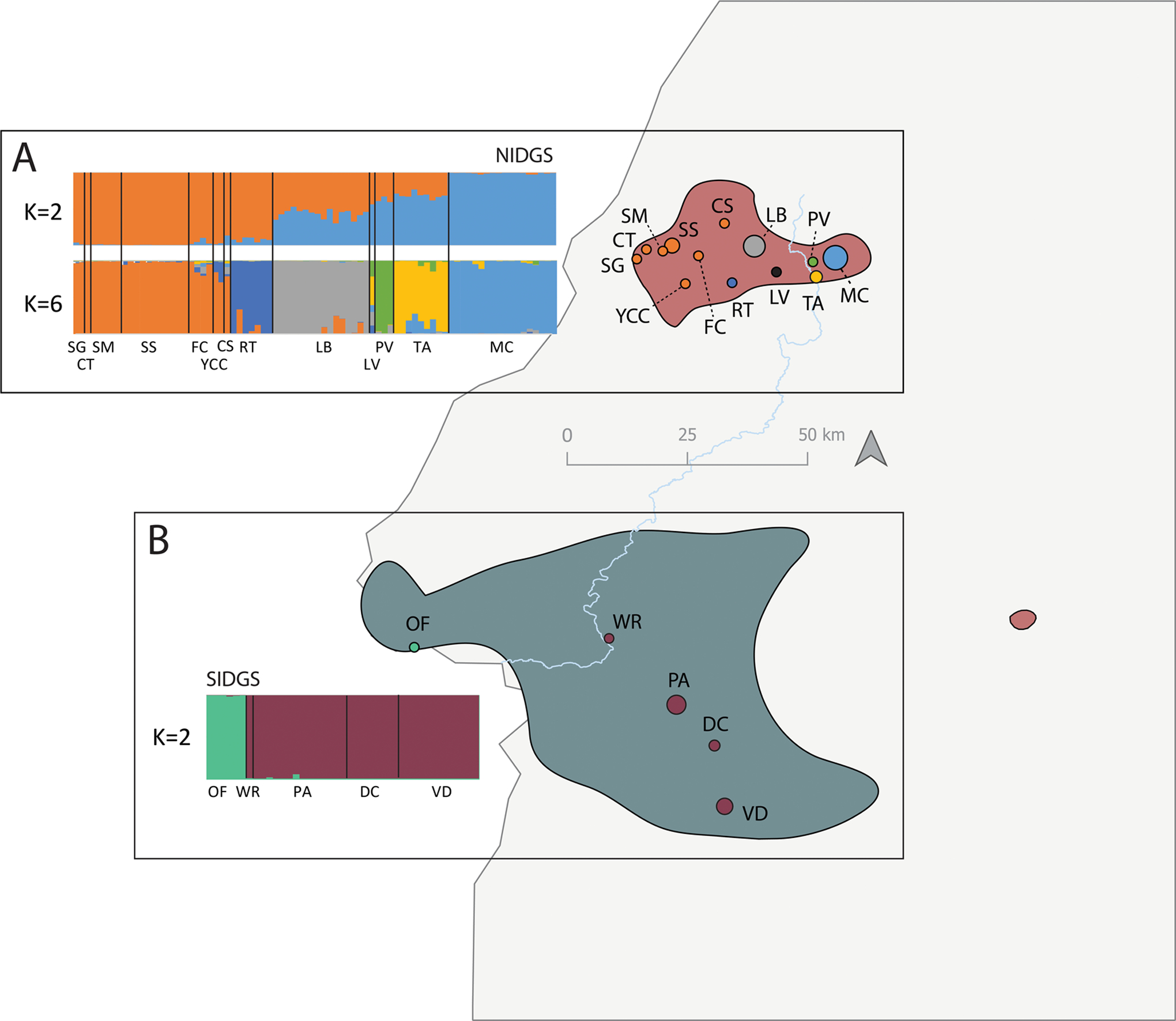
Population structure analyses and conservation unit delimitation for the NIDGS (A) and SIDGS (B). STRUCTURE barplots represent the most supported K (K = 2) for the neutral datasets using the Evanno method, after excluding loci deviating from HWE. For NIDGS, we further included K = 6, as the second most supported K, as it also provided biologically meaningful results. Populations on the map are colored according to the largest proportion of assignment to a given K population based on K = 6 in NIDGS and K = 2 in SIDGS. For NIDGS, the population LV is colored black due to multiple mixed ancestry. Within each species, different colors match the STRUCTURE plot population symbols represent. Locality codes refer to localities listed in Table 1. Background red and blue areas represent the distribution of NIDGS and SIDGS, respectively. The light blue and gray lines represents the Weiser River and the Idaho state border, respectively.

In terms of population differentiation, at the interspecific level, average F_ST between NIDGS and SIDGS was 0.143, compared to 0.05 and 0.100 within NIDGS and SIDGS for the same dataset, respectively. At the intraspecific level and considering the SIDGS dataset separately, average neutral pairwise F_ST was highest for Olds Ferry (0.13), considerably higher than the average value of 0.04 (Figure S11C, Supporting information). However, as seen in the SIDGS adaptive PCA, Paddock was the most distinct population and also had the highest average pairwise F_ST (0.24), considerably higher than the average value of 0.15 (Figure S11D, Supporting information).

Considering the levels of genetic diversity, for the IDGS dataset, no NIDGS population showed significantly decreased H_O compared to H_E, but Lower Butter did show significantly higher H_O than H_E (Table 4). Contrarily, for the same dataset, two out of four SIDGS populations showed significantly lower H_O than H_E. SIDGS populations tended to have significantly lower H_E than NIDGS populations (Table S1, Supporting information). At the intraspecific level, for NIDGS we observed an average of neutral H_O (and H_E) 0.279 (0.300) and 0.270 (0.301) for west and east metapopulations, respectively (Table 4). At the adaptive level, we observed an average H_O (and H_E) of 0.170 (0.178) and 0.244 (0.313) for west and east metapopulations, respectively (Table 4). Genetic diversity was not significantly different between metapopulations at the neutral level, but was significantly lower in west at the adaptive level. Additionally, neutral diversity was significantly higher than adaptive diversity in both metapopulations. For the SIDGS, we observed an average of neutral H_O (and H_E) of 0.288 (0.287) and 0.219 (0.277) for west and east metapopulations, respectively (Table 4). The east metapopulation showed significantly lower genetic diversity at both the neutral (only H_O) and adaptive (only H_E) levels, as well as significantly lower genetic diversity at the neutral compared to the adaptive level (both H_O and H_E).

Table 4.

Genetic diversity per population, estimated as observed and expected heterozygosity (H_O and H_E, respectively) for the total dataset of the IDGS (‘Interspecific’) and for the neutral and adaptive datasets of the NIDGS and SIDGS (‘Intraspecific’), with indication of the number of samples per population (N). We additionally report neutral and adaptive H_O/H_E for IDGS metapopulations (east and west) at the intraspecific level. Bold H_O/H_E pairs represent comparisons that were significantly different at p < 0.05. Dashes indicate that no estimate was made due to sample size. Estimates of H_O with N = 1 represent individual heterozygosity as a proxy for population heterozygosity.

	Interspecific					Intraspecific
		Total					Neutral		Adaptive
Population	N	π	PA	H O	H E	N	H O	H E	H O	H E
NIDGS
west
Cap Gun/Tree Farm (CT)	0	-	-	-	-	1	0.162	-	0.161	-
Cold Springs (CS)	0	-	-	-	-	1	0.210	-	0.167	-
Fawn Creek (FC)	0	-	-	-	-	4	0.244	0.273	0.228	0.220
Huckleberry (HU)	0	-	-	-	-	0	-	-	-	-
Summit Gulch (SG)	1	0.200	0	0.128	-	2	0.188	0.278	0.140	0.182
Squirrel Manor (SM)	2	0.226	1	0.141	0.140	5	0.253	0.290	0.145	0.214
Steve’s Creek/Squirrel Valley (SS)	11	0.243	66	0.152	0.148	11	0.309	0.305	0.177	0.168
YCC	1	0.209	0	0.134	-	2	0.226	0.275	0.194	0.200
total						26	0.279	0.300	0.170	0.178
east
Lost Valley (LV)	1	0.187	1	0.106	-	1	0.211	-	0.193	-
Lower Butter (LB)	11	0.227	37	0.147	0.138	16	0.269	0.278	0.272	0.263
Mud Creek (MC)	17	0.225	60	0.136	0.130	18	0.280	0.286	0.190	0.175
Price Valley (PV)	3	0.189	2	0.115	0.125	3	0.197	0.259	0.126	0.207
Rocky Top (RT)	6	0.221	23	0.140	0.132	7	0.253	0.258	0.324	0.294
Slaughter Gulch (SL)	0	-	-	-	-	0	-	-	-	-
Tamarack (TA)	8	0.236	23	0.141	0.140	9	0.285	0.296	0.264	0.270
total						54	0.270	0.301	0.244	0.313
SIDGS
west
Olds Ferry (OF)	3	0.188	76	0.133	0.124	6	0.288	0.287	0.265	0.251
east
Dry Creek (DC)	3	0.156	11	0.100	0.136	8	0.167	0.268	0.197	0.210
Paddock (PA)	9	0.196	83	0.123	0.133	14	0.237	0.283	0.382	0.410
Van Deusen (VD)	4	0.187	17	0.122	0.127	12	0.225	0.263	0.183	0.226
Weiser River (WR)	0	-	-	-	-	1	0.235	-	0.133	-
total						35	0.219	0.277	0.281	0.403

Discussion

We examined the genetic basis of adaptive divergence between two endemic and vulnerable sister species of Idaho ground squirrels and assessed the diversity and differentiation at both neutral and adaptive loci among populations of each species. We found that combining different methods to identify adaptive variation is useful to address adaptive differentiation across the speciation continuum, particularly in recently diverged species, which can be subject to strong and heterogeneous local adaptation among populations within species (Luikart et al. 2019). Additionally, we found that environmental association analyses (EAAs) generally led to the detection of a larger number of candidate loci. EAAs have more power to detect loci associated with polygenic adaptation, and are fairly robust to the confounding effects of demography, compared to outlier detection methods (Ahrens et al. 2018; Dalongeville et al. 2018).

Comparing the analyses at the inter- and intraspecific level, we found that there were more differences between than within species regarding the association to specific environmental conditions; these differences were consistent both before and after controlling for collinearity with demographic history. At the intraspecific level, more heterogeneous environments promoted increased adaptive differentiation between populations. This was true both in cases where populations were distinct at the neutral (demographic) level, and in cases where they were not. Understanding patterns of both neutral and adaptive genetic diversity across a species range is important for conservation and management, particularly in the current context of increasing habitat and environmental change (Teixeira & Huber 2021; DeWoody et al. 2021).

Our work highlights the complex dynamics of inter- and intraspecific differentiation of two closely related small mammal species that are highly susceptible to environmental and habitat change.

(dis)Agreement between adaptive loci detection methods

In this study we used multiple methods to identify putatively adaptive loci at the interspecific level. Considering sets of loci detected by multiple methods is a conservative approach for identifying loci associated with local adaptation, while avoiding being overly conservative (Garcia-Elfring et al. 2019). The low overlap between loci identified across detection methods is likely related to the different assumptions and algorithms underlying the different methods (Ahrens et al. 2018; Capblancq et al. 2018; Dalongeville et al. 2018).

While the outlier approach provides an overview regarding overall single SNP differentiation above what is expected from neutrality, the different GEAs identify loci associated with environmental variables, and are thus more likely be informative on patterns of local adaptation (Hoban et al. 2016; Forester, Lasky, et al. 2018). With the outlier detection method (pcadapt), we found a clear separation between species at the adaptive level, which might be related to ecological differentiation of the two IDGS species (Nosil et al. 2009; McEwen et al. 2013). Still, the observed adaptive differentiation could partially result from collinearity with demographic processes and associated genetic drift, given that outlier detection methods do not explicitly exclude population structure from the analysis, and different GEAs account for it in different ways and based on different assumptions (Seehausen et al. 2014; Forester, Lasky, et al. 2018; Ahrens et al. 2018). For the LFMM and RDA analyses, the causal factors driving differentiation between species (e.g. neutral or adaptive processes or some combination) also cannot be easily disentangled due to collinearity between environment and demography at the interspecific level (Ahrens et al. 2018). However, these two analyses perform better at identifying adaptive variation when selection gradients are weakly correlated with population structure (Capblancq et al. 2018). The adaptive patterns found by the two multivariate GEAs (RDA and pRDA) were very similar, even though the pRDA explicitly excluded the effect of population structure. This congruence might be related to the fact that, in RDAs, the rates of false positives tend to be lower when allele frequencies show high correlations with ecological variables (Frichot et al. 2015). Thus, despite a clear effect of population structure in the data, the identified SNPs seem to overlap strongly with analyses that control for demographic patterns.

Although we did not find particular Gene Ontology terms associated with putative functions of adaptive genes in our analysis, we found two non-synonymous substitutions in known genes identified by the interspecific RDA, one of which was also identified by pcadapt, the NPR1. This gene has been found to be highly expressed in brown adipose tissue of thirteen-lined ground squirrels during hibernation, relating to heat production during periodic arousals from hypothermic torpor (Hampton et al. 2013). Adaptations relating to adipose tissue are common in high altitude adapted rodents (Gossmann et al. 2019), and these associations suggest that there are adaptive differences between IDGS species relating to their torpor patterns. In fact, one study on Columbian ground squirrel (Urocitellus columbianus) found that emergence timing was heritable and hence, squirrels’ emergence date may also reflect local adaptations (Lane et al. 2011). Altitude differences might have resulted in adaptive differences between NIDGS and SIDGS in production and storage of fat, and increased metabolism and oxygen transport at higher elevations, as seen in other mammals (Faherty et al. 2018; Waterhouse et al. 2018; Werhahn et al. 2018; Garcia-Elfring et al. 2019).

Differentiation of recently diverged species vs. populations

As in previous studies (Garner et al. 2005; Hoisington 2007; Hoisington-Lopez et al. 2012), we observed a clear genetic separation between NIDGS and SIDGS. This separation was clear at both the neutral and adaptive levels, which is a common pattern observed in ecologically divergent groups that are evolving in allopatry (Nosil et al. 2009). We found more loci associated with environmental variables among the two species of IDGS (340 SNPs) than within NIDGS (150 SNPs) and SIDGS (18 SNPs). These results show that adaptive differences between species are more numerous and likely more scattered across the genome compared to adaptive differences within species (Nosil & Feder 2013). Additionally, the initial adaptive or nonadaptive vicariance of the two species has evolved into what can now be considered ecological speciation (Rundell & Price 2009). These patterns point to a process of speciation originated from the vicariance of the two IDGS groups with gradually reduced gene flow, increased neutral genetic drift, and subsequent ecological divergence (and potential reproductive isolation) as a result of local adaptation (Nosil et al. 2009; Rundell & Price 2009). While the outlier detection analyses identified a clear separation between the two species, the GEA analyses pointed to a distinction of particular populations within species, which might also relate to an inflated rate of false negatives that is common when environmental distance is correlated with genetic distance (Ahrens et al. 2018). Thus, although GEAs account for and correct analyses for population structure, we found that hierarchical approaches, such as the one used here, are essential in the presence of multiple levels of genetic structure.

Within species, we identified different clustering of populations when considering neutral and adaptive variation separately. This suggests that local adaptation and demographic processes are both important and act independently in shaping genetic variation in IDGS. We found evidence for six different demographic units based on PCA and STRUCTURE analyses of neutral loci in NIDGS. As seen in other small mammals with historically reduced ranges across altitudinal gradients (Waterhouse et al. 2018; Bi et al. 2019), the higher differentiation observed among east NIDGS populations may result from loss of suitable habitat and dispersal corridors between populations, currently leading to the isolation of populations (Yensen 1999; Gavin et al. 1999; Sherman & Runge 2002; Barrett 2005). In contrast, the higher homogeneity seen in west NIDGS populations might reflect both higher connectivity among populations, and assisted gene flow from translocations in the late 1990s (Gavin et al. 1998; Sherman & Gavin 1999). This result is similar to that of previous microsatellite analyses for the eastern part of the range although this study did not analyze the exact same populations (Garner et al. 2005). However, it somewhat contrasts with our hypothesis of IBD and the results of an allozyme study, which found significant IBD within the western region (Gavin et al. 1999), and with unpublished results from Hoisington (2007) which found evidence for additional substructure and restricted gene flow within both the eastern and western groups. For SIDGS, the neutral dataset identified two genetic groups with the highest differentiation between populations on different sides of the Weiser River, which corroborates previous studies (Garner et al. 2005; Hoisington 2007; Zero et al. 2017). Interestingly, although Olds Ferry was the most distinct population at the neutral level, it was not substantially differentiated from other populations on the eastern side of the Weiser River at the adaptive level, suggesting that its distinction is mostly due to demographic (i.e. neutral) processes (Garner et al. 2005; Hoisington-Lopez et al. 2012; Zero et al. 2017).

Overall, we saw that some populations that were differentiated at the neutral level, were also distinct at the adaptive level (e.g. Lower Butter), others that were differentiated at the neutral level were not found to be distinct at the adaptive level (e.g. Mud Creek, Olds Ferry), and others were more distinct at the adaptive than the neutral level (Rocky Top and Paddock). In SIDGS, no populations were distinct at both the neutral and adaptive level. This suggests that population isolation in SIDGS might not be as strong as in NIDGS and thus only populations undergoing strong selective pressure are currently locally adapted in SIDGS (Funk et al. 2012; Tigano & Friesen 2016). Although neutral genetic diversity is regarded as an important proxy for population health (DeWoody et al. 2021), recent studies argue for increased consideration of ecologically meaningful diversity, which might be essential for effective conservation strategies (Ralls et al. 2018; Teixeira & Huber 2021). These results highlight the importance of considering different types of loci for conservation management and also to guide additional research on this species, as populations that are distinct at only the neutral or adaptive level, or that are distinct at both levels, will likely represent different types of conservation units, and contribute differently to the species adaptive potential (Funk et al. 2012; Razgour et al. 2019).

High landscape heterogeneity leads to clearer patterns of intraspecific local adaptation

Intraspecific adaptive differences can quickly arise in populations that become isolated and/or that are distributed across highly variable environmental gradients (Doebeli & Dieckmann 2003; Smith et al. 2019). Small populations can naturally become locally adapted during the process of isolation, resulting in a gradual increase in adaptive differentiation from other populations, compared to neutral differentiation (Doebeli & Dieckmann 2003; Holderegger et al. 2006; Wood et al. 2016). Thus, there is an important role of adaptive variants and their specific adaptations in the maintenance of genetic diversity and the long-term persistence of threatened species (Rubidge et al. 2012). From our results, most SIDGS populations were associated with a similar set of environmental variables, while there were no generalizable associations common to most NIDGS populations. These differences are within our expectations of adaptive differentiation between the two species, given that NIDGS occur at more heterogeneous landscapes than SIDGS, mainly in relation to elevation (Yensen 1991; Hoisington-Lopez et al. 2012).

NIDGS showed a higher number of distinct populations at both the neutral and adaptive level, with Rocky Top and Lower Butter as the most distinct populations. Interestingly, these are the highest elevation populations sampled in this study but not the highest documented populations for the species. No population showed particularly low genetic diversity, indicating that NIDGS populations are unique but are not being affected by inbreeding or extensive drift, despite local bottlenecks (Assis et al. 2013). The emergence of particular adaptations to elevation in NIDGS populations was potentially promoted by a decrease in gene flow, a pattern also observed in other North American ground squirrels (Hodgson et al. 2011; Eastman et al. 2012). Genomic signatures of adaptive differences within NIDGS might reflect associations with timing of snowmelt and site productivity, respectively, which are known to influence torpor timing (Hoisington-Lopez et al. 2012; Zero et al. 2017; Goldberg, Conway, Evans Mack, et al. 2020). The highest adaptive differentiation in SIDGS was observed for Paddock, although it was not distinct at the neutral level from other populations on the same side of the Weiser River, which is indicative of strong selection in this population despite generalized gene flow among east SIDGS populations (Tigano & Friesen 2016).

The results of the intraspecific GEAs appear to highlight particular adaptive responses as a result of local adaptation facilitated by demographic isolation in NIDGS, while in SIDGS the patterns appear to match local adaptation despite low levels of demographic differentiation. In the face of gene flow, local adaptation depends upon various factors including the strength of selection on the trait and the migration rate, which needs to be considered for effective conservation (Tigano & Friesen 2016; Razgour et al. 2018).

Conservation recommendations

Both IDGS species have undergone accentuated population declines in the last 50 years (Yensen 1999; Gavin et al. 1999; Evans Mack 2003), suggesting high susceptibility to environmental and landscape changes. As a result, NIDGS were listed as threatened under the federal Endangered Species Act (ESA) in 2000 (USFWS 2000), and as Critically Endangered by the International Union for Conservation of Nature (Hafner et al. 1998). SIDGS are listed as Vulnerable by the IUCN (IUCN 2018) and were a former candidate for listing under the ESA, although they were ultimately not listed. The decline of these two species has resulted in metapopulations approaching a state of nonequilibrium, where many populations became small and isolated, and thus especially prone to both diversification and extinction (Harrison & Taylor 1997; Hanski & Gaggiotti 2004; Pironon et al. 2017). Metapopulations can retain genetic variation more readily than simply isolated subpopulations from a once panmictic population, and can be more resilient to extinction due to their intrinsic colonization-extinction-recolonization dynamics (Nee & May 1992; Levin 1995; Gavrilets et al. 2000). However, this resilience is dependent on how many individuals and how much genetic diversity each subpopulation maintains (Fahrig & Merriam 1994; Furlan et al. 2020). Our results showed that west NIDGS populations are genetically more homogenous based on low and mostly non-significant levels of pairwise F_ST, but east NIDGS form a more fragmented patch network. Interestingly, levels of neutral genetic diversity in NIDGS were not different between west and east metapopulations, but were significantly lower in the west at the adaptive level. These results suggest that the habitat and environmental conditions are more homogeneous in the west region, but could also suggest a decrease in the signal of local adaptation due to translocations (Pacioni et al. 2019). For SIDGS, east populations were significantly less diverse at the neutral level than in the west (for which we only sampled one population), suggesting that east populations have been subjected to stronger declines (Weeks et al. 2011). Translocations among west NIDGS populations (Sherman & Gavin 1999; Gavin et al. 1999) and among east SIDGS populations (Yensen et al. 2010; Yensen & Tarifa 2012) were performed to supplement small and isolated populations, and might have led to an increased level of genetic homogeneity at the neutral level (Weeks et al. 2011; Landguth & Balkenhol 2012).

Translocations generally lead to an overall maintenance of genetic diversity with consequent improved survival for the species, by spreading the extinction risk across multiple populations; however, there is a trade-off regarding the maintenance of local adaptation (Furlan et al. 2020). Most conservation oriented translocations have resulted in beneficial intended consequences, namely in preventing extinction (Novak et al. 2021), but simulations suggest that translocations are most effective if performed multiple times, particularly for the establishment of new populations (Pacioni et al. 2019). Successful translocations would result in increased genetic diversity and low neutral and adaptive differentiation (White et al. 2018), but previous studies have found low rates of translocation success, particularly in SIDGS (Panek 2005; Busscher 2009; Yensen et al. 2010; Smith et al. 2019). Significant differences in timing of torpor emergence have been seen in Columbian ground squirrels translocated to populations with different phenology, potentially leading to changes in fitness of translocated individuals (Lane et al. 2019). This could be related to an effect of strong local adaptation in source populations, resulting in low success in the establishment of new populations in environmentally distinct areas (Hedrick 1995). In cases where closely located populations are not available, and thus local adaptation could be compromised by translocations, it is still advisable to consider translocations if the impact of low effective population size and genetic drift will result in population extinction (Weeks et al. 2011). Thus, although there is some indication that translocations have maintained neutral genetic diversity in west NIDGS populations, further work is necessary to verify the impact of translocation in east SIDGS by sampling source populations. This is especially important as, in line with previous microsatellite work (Garner et al. 2005; Hoisington-Lopez et al. 2012), SIDGS populations were generally less genetically diverse than NIDGS, which could be the result of effects of past bottlenecks and genetic drift (Rousset & Raymond 1995), and points to the need of increased protection of this species (Garner et al. 2005).

Our results provide an important baseline for further work that aims to develop management strategies in response to land use and habitat changes (Henry & Russello 2013). Further sampling is required to validate the results of those populations with lower number of samples, given that adaptive variation is less likely to be detected with low sample sizes (Lotterhos & Whitlock 2015). The inclusion of additional populations would also be ideal, not only for confirming the patterns found in this study, but also for identifying other conservation units that might warrant special protection.

High Throughput Sequencing of minimally invasive samples

We made use of a minimally invasive sampling method, in order to minimize the impact of sampling on populations (Carroll et al. 2018). Buccal swabs, as used in this study, have been specifically used in high throughput sequencing (HTS) genotyping using targeted sequencing (Chang et al. 2007; McMichael et al. 2009), and have been shown to allow for non-targeted HTS genotyping, such as RAD sequencing, in amphibians (Peek et al. 2019). To our knowledge, this is the first study genotyping buccal swabs from a mammal with a non-targeted HTS approach, adding to the growing literature aiming to use less invasive sampling strategies to examine genomic variation in species of conservation concern (Andrews et al. 2018; Carroll et al. 2018). Buccal swabbing may provide an ideal data collection method for numerous species that require non-invasive techniques (i.e. species of conservation concern) but where more traditionally used methods such as hair snares are not ideal. For instance, there are 330 rodent species in the world (besides IDGS) currently listed as vulnerable, endangered or critically endangered according to the IUCN Red List (IUCN 2012). Most of these species exist in small isolated populations where further information regarding adaptive differences could potentially provide useful information with regards to recovery efforts and metapopulation dynamics. However, our sample genotyping success was low due to low DNA yield, typical of minimally invasive sampling, and thus studies considering using buccal swabs should conduct pilot studies to determine DNA yield and be aware of this limitation.

Conclusions

In this study, we examined two rare and recently diverged species of ground squirrels, identifying multiple sets of new loci with around 3000 SNPs each using minimally invasive sampling methods. Our results corroborate previous studies regarding the clear differentiation between NIDGS and SIDGS and provide further details regarding the differentiation of these two sister species at the adaptive level. We additionally analyzed the demographic and adaptive variation of each species independently and determined that local adaptation played a more prominent role in differentiation among NIDGS populations, while geographic barriers appear to be the largest determinant of genetic differentiation in SIDGS. Identifying appropriate conservation units within both species will require further investigation with more samples and including additional populations, in particular the geographically disjunct Round Valley population at the southern extent of range (Figure 1) that was previously identified as genetically distinct (Hoisington 2007; Hoisington-Lopez et al. 2012). However, we are the first to identify adaptive loci that distinguish not only the two species, but also distinguish among populations within each species, and the associations of these adaptive loci with environmental variables. The differences we detected will potentially help inform management plans aiming to protect the evolutionary and adaptive capacity of populations. Our results suggest clear metapopulation structure in both species with strong isolation-by-distance (and potentially isolation-by-barriers), as well as evidence of recent local adaption within some of these small and isolated metapopulations. Furthermore, these new collection techniques for mammals combined with our analysis provide a road map for future studies who aim to collect similar information from other small mammal populations.

Data Accessibility

Raw reads and mapped bam files for the total 304 ground squirrels are available on NCBI’s BioProject PRJNA747996. Additional meta-data for each individual ground squirrel, including respective scores for all environmental variables tested, as well as the final three VCF files used for all analyses with respective R code employed can be found in DRYAD (https://doi.org/10.5061/dryad.sj3tx965c).

References

- Ahrens CW, Rymer PD, Stow A et al. (2018) The search for loci under selection: trends, biases and progress. Molecular Ecology, 27, 1342–1356. [DOI] [PubMed] [Google Scholar]
- Ali OA, O’Rourke SM, Amish SJ et al. (2016) RAD capture (Rapture): flexible and efficient sequence-based genotyping. Genetics, 202, 389–400. [DOI] [PMC free article] [PubMed] [Google Scholar]
- Andrews KR, De Barba M, Russello MA, Waits LP (2018) Advances in Using Non-invasive, Archival, and Environmental Samples for Population Genomic Studies. In: Population Genomics, pp. 1–37. Springer, Cham. [Google Scholar]
- Andrews KR, Good JM, Miller MR, Luikart G, Hohenlohe PA (2016) Harnessing the power of RADseq for ecological and evolutionary genomics. Nature Reviews Genetics, 17, 81–92. [DOI] [PMC free article] [PubMed] [Google Scholar]
- Assis J, Castilho Coelho N, Alberto F et al. (2013) High and distinct range-edge genetic diversity despite local bottlenecks. PLoS One, 8, e68646. [DOI] [PMC free article] [PubMed] [Google Scholar]
- Baird NA, Etter PD, Atwood TS et al. (2008) Rapid SNP discovery and genetic mapping using sequenced RAD markers. PLoS One, 3, e3376. [DOI] [PMC free article] [PubMed] [Google Scholar]
- Barrett JS (2005) Population Viability of the Southern Idaho Ground Squirrel (Spermophilus brunneus endemicus): Effects of an Altered Landscape. Unpublished thesis. Boise State University. [Google Scholar]
- Bateman A (2019) UniProt: A worldwide hub of protein knowledge. Nucleic Acids Research, 47, D506–D515. [DOI] [PMC free article] [PubMed] [Google Scholar]
- Besnier F, Glover KA (2013) ParallelStructure: A R package to distribute parallel runs of the population genetics program STRUCTURE on multi-core computers (M Anisimova, Ed,). PLoS One, 8, e70651. [DOI] [PMC free article] [PubMed] [Google Scholar]
- Bi K, Linderoth T, Singhal S et al. (2019) Temporal genomic contrasts reveal rapid evolutionary responses in an alpine mammal during recent climate change. PLoS Genetics, 15, e1008119. [DOI] [PMC free article] [PubMed] [Google Scholar]
- Burak GS (2011) Status review for northern Idaho ground squirrel (Spermophilus brunneus brunneus). U.S. Fish and Wildlife Service, Region 1, Idaho Fish and Wildlife Office, Boise, ID. [Google Scholar]
- Busscher KL (2009) Improving Success of Translocating Southern Idaho Ground Squirrels (Spermophilus endemicus). Boise State University. [Google Scholar]
- Capblancq T, Luu K, Blum MGB, Bazin E (2018) Evaluation of redundancy analysis to identify signatures of local adaptation. Molecular Ecology Resources, 18, 1223–1233. [DOI] [PubMed] [Google Scholar]
- Carroll EL, Bruford MW, DeWoody JA et al. (2018) Genetic and genomic monitoring with minimally invasive sampling methods. Evolutionary Applications, 11, 1094–1119. [DOI] [PMC free article] [PubMed] [Google Scholar]
- Catchen J, Hohenlohe PA, Bassham S, Amores A, Cresko WA (2013) Stacks: an analysis tool set for population genomics. Molecular Ecology, 22, 3124–3140. [DOI] [PMC free article] [PubMed] [Google Scholar]
- Chang ML, Terrill RL, Bautista MM et al. (2007) Large-scale SNP genotyping with canine buccal swab DNA. Journal of Heredity, 98, 428–437. [DOI] [PubMed] [Google Scholar]
- Chen H, Boutros PC (2011) VennDiagram: a package for the generation of highly-customizable Venn and Euler diagrams in R. BMC Bioinformatics, 12, 35. [DOI] [PMC free article] [PubMed] [Google Scholar]
- Dalongeville A, Benestan L, Mouillot D, Lobreaux S, Manel S (2018) Combining six genome scan methods to detect candidate genes to salinity in the Mediterranean striped red mullet (Mullus surmuletus). BMC Genomics, 19, 217. [DOI] [PMC free article] [PubMed] [Google Scholar]
- Danecek P, Auton A, Abecasis G et al. (2011) The variant call format and VCFtools. Bioinformatics, 27, 2156–2158. [DOI] [PMC free article] [PubMed] [Google Scholar]
- DeWoody JA, Harder AM, Mathur S, Willoughby JR (2021) The long‐standing significance of genetic diversity in conservation. Molecular Ecology, in press. [DOI] [PubMed] [Google Scholar]
- Doebeli M, Dieckmann U (2003) Speciation along environmental gradients. Nature, 421, 259–264. [DOI] [PubMed] [Google Scholar]
- Eastman LM, Morelli TL, Rowe KC, Conroy CJ, Moritz C (2012) Size increase in high elevation ground squirrels over the last century. Global Change Biology, 18, 1499–1508. [Google Scholar]
- Evanno G, Regnaut S, Goudet J (2005) Detecting the number of clusters of individuals using the software STRUCTURE: a simulation study. Molecular Ecology, 14, 2611–2620. [DOI] [PubMed] [Google Scholar]
- Evans Mack D (2003) Northern Idaho ground squirrel population monitoring 2003 annual report. Idaho Department of Fish and Game, McCall, ID. [Google Scholar]
- Faherty SL, Villanueva-Cañas JL, Blanco MB, Albà MM, Yoder AD (2018) Transcriptomics in the wild: hibernation physiology in free-ranging dwarf lemurs. Molecular Ecology, 27, 709–722. [DOI] [PubMed] [Google Scholar]
- Fahrig L, Merriam G (1994) Conservation of fragmented populations. Conservation Biology, 8, 50–59. [Google Scholar]
- Fišer C, Robinson CT, Malard F (2018) Cryptic species as a window into the paradigm shift of the species concept. Molecular Ecology, 27, 613–635. [DOI] [PubMed] [Google Scholar]
- Fletcher NK, Acevedo P, Herman JS et al. (2019) Glacial cycles drive rapid divergence of cryptic field vole species. Ecology and Evolution, 9, 1–13. [DOI] [PMC free article] [PubMed] [Google Scholar]
- Forester BR, Landguth EL, Hand BK, Balkenhol N (2018) Landscape Genomics for Wildlife Research. In: Population Genomics, pp. 1–40. Springer, Cham. [Google Scholar]
- Forester BR, Lasky JR, Wagner HH, Urban DL (2018) Comparing methods for detecting multilocus adaptation with multivariate genotype-environment associations. Molecular Ecology, 27, 2215–2233. [DOI] [PubMed] [Google Scholar]
- French AR (1982) Intraspecific differences in the pattern of hibernation in the ground squirrel Spermophilus beldingi. Journal of Comparative Physiology, 148, 83–91. [Google Scholar]
- Frichot E, Schoville SD, De Villemereuil P, Gaggiotti OE, François O (2015) Detecting adaptive evolution based on association with ecological gradients: Orientation matters! Heredity, 115, 22–28. [DOI] [PMC free article] [PubMed] [Google Scholar]
- Friis G, Fandos G, Zellmer AJ et al. (2018) Genome-wide signals of drift and local adaptation during rapid lineage divergence in a songbird. Molecular Ecology, 27, 5137–5153. [DOI] [PubMed] [Google Scholar]
- Funk WC, McKay JK, Hohenlohe PA, Allendorf FW (2012) Harnessing genomics for delineating conservation units. Trends in Ecology and Evolution, 27, 489–496. [DOI] [PMC free article] [PubMed] [Google Scholar]
- Furlan EM, Gruber B, Attard CRM et al. (2020) Assessing the benefits and risks of translocations in depauperate species: A theoretical framework with an empirical validation. Journal of Applied Ecology, 57, 831–841. [Google Scholar]
- Garcia-Elfring A, Barrett RDH, Millien V (2019) Genomic signatures of selection along a climatic gradient in the northern range margin of the white-footed mouse (Peromyscus leucopus). Journal of Heredity, 110, 684–695. [DOI] [PubMed] [Google Scholar]
- Garner A, Rachlow JL, Waits LP (2005) Genetic diversity and population divergence in fragmented habitats: conservation of Idaho ground squirrels. Conservation Genetics, 6, 759–774. [Google Scholar]
- Gavin TA, Sherman PW, Yensen E (1998) Translocation and inventory of northern Idaho ground squirrels (Spermophilus brunneus brunneus) in 1998. Cornell University, Ithaca, New York, and Albertson College, Caldwell, Idaho. [Google Scholar]
- Gavin TA, Sherman PW, Yensen E, May B (1999) Population genetic structure of the northern Idaho ground squirrel (Spermophilus brunneus brunneus). Journal of Mammalogy, 80, 156–168. [Google Scholar]
- Gavrilets S, Acton R, Gravner J (2000) Dynamics of speciation and diversification in a metapopulation. Evolution, 54, 1493–1501. [DOI] [PubMed] [Google Scholar]
- Gill AE, Yensen E (1992) Biochemical differentiation in the Idaho ground squirrel Spermophilus brunneus (Rodentia: Sciuridae). Great Basin Natura, 52, 155–159. [Google Scholar]
- Goldberg AR, Conway CJ (2021) Hibernation behavior of a federally threatened ground squirrel: climate change and habitat selection implications. Journal of Mammalogy, 102, 574–587. [Google Scholar]
- Goldberg AR, Conway CJ, Evans Mack D, Burak G (2020) Winter versus Summer habitat selection in a threatened ground squirrel. Journal of Wildlife Management, 84, 1548–1559. [Google Scholar]
- Goldberg AR, Conway CJ, Tank DC et al. (2020) Diet of a rare herbivore based on DNA metabarcoding of feces: Selection, seasonality, and survival. Ecology and Evolution, 10, 7627–7643. [DOI] [PMC free article] [PubMed] [Google Scholar]
- Gossmann TI, Shanmugasundram A, Börno S et al. (2019) Ice-Age climate adaptations trap the alpine marmot in a state of low genetic diversity. Current Biology, 29, 1712–1720. [DOI] [PMC free article] [PubMed] [Google Scholar]
- Goudet J (2005) hierfstat, a package for r to compute and test hierarchical F-statistics. Molecular Ecology Notes, 5, 184–186. [Google Scholar]
- Hafner DJ, Kirkland GL, Yensen E (1998) North American Rodents: Status Survey and Conservation Action Plan. IUCN/SSC Rodent Specialist Group, Gland, Switzerland and Cambridge, UK. [Google Scholar]
- Hampton M, Melvin RG, Andrews MT (2013) Transcriptomic analysis of brown adipose tissue across the physiological extremes of natural hibernation (K Dahlman-Wright, Ed,). PLoS One, 8, e85157. [DOI] [PMC free article] [PubMed] [Google Scholar]
- Hanski I (1998) Metapopulation dynamics. Nature, 396, 41–49. [Google Scholar]
- Hanski I, Gaggiotti OE (2004) Ecology, Genetics, and Evolution of Metapopulations. Elsevier Academic Press, Burlington, MA, USA. [Google Scholar]
- Harrison S, Taylor AD (1997) Empirical evidence for metapopulation dynamics. In: Metapopulation Biology: Ecology, Genetics, and Evolution (eds Hanski I, Gilpin M), pp. 27–42. Academic Press, San Diego, CA, USA. [Google Scholar]
- Hedrick PW (1995) Gene flow and genetic restoration: the Florida panther as a case study. Conservation Biology, 9, 996–1007. [DOI] [PubMed] [Google Scholar]
- Helgen KM, Cole FR, Helgen LE, Wilson DE (2009) Generic revision in the Holarctic ground squirrel genus Spermophilus. Journal of Mammalogy, 90, 270–305. [Google Scholar]
- Helmstetter NA, Conway CJ, Stevens BS, Goldberg AR (2021) Balancing transferability and complexity of species distribution models for rare species conservation. Diversity and Distributions, 27, 95–108. [Google Scholar]
- Henry P, Russello MA (2013) Adaptive divergence along environmental gradients in a climate-change-sensitive mammal. Ecology and Evolution, 3, 3906–3917. [DOI] [PMC free article] [PubMed] [Google Scholar]
- Hoban S, Kelley JL, Lotterhos KE et al. (2016) Finding the genomic basis of local adaptation: pitfalls, practical solutions, and future directions. The American Naturalist, 188, 379–397. [DOI] [PMC free article] [PubMed] [Google Scholar]
- Hodgson JA, Moilanen A, Wintle BA, Thomas CD (2011) Habitat area, quality and connectivity: striking the balance for efficient conservation. Journal of Applied Ecology, 48, 148–152. [Google Scholar]
- Hoffmann AA, Sgrò CM, Kristensen TN (2017) Revisiting adaptive potential, population size, and conservation. Trends in Ecology and Evolution, 32, 506–517. [DOI] [PubMed] [Google Scholar]
- Hoisington-Lopez JL, Waits LP, Sullivan J (2012) Species limits and integrated taxonomy of the Idaho ground squirrel (Urocitellus brunneus): genetic and ecological differentiation. Journal of Mammalogy, 93, 589–604. [Google Scholar]
- Hoisington J (2007) Conservation genetics, landscape genetics and systematics of the two subspecies of the endemic Idaho groud squirrel (Spermophilus brunneus). PhD Thesis, University of Idaho. [Google Scholar]
- Holderegger R, Kamm U, Gugerli F (2006) Adaptive vs. neutral genetic diversity: implications for landscape genetics. Landscape Ecology, 21, 797–807. [Google Scholar]
- Hope AG, Malaney JL, Bell KC et al. (2016) Revision of widespread red squirrels (genus: Tamiasciurus) highlights the complexity of speciation within North American forests. Molecular Phylogenetics and Evolution, 100, 170–182. [DOI] [PubMed] [Google Scholar]
- Hope AG, Panter N, Cook JA, Talbot SL, Nagorsen DW (2014) Multilocus phylogeography and systematic revision of North American water shrews (genus: Sorex). Journal of Mammalogy, 95, 722–738. [Google Scholar]
- Hope AG, Stephens RB, Mueller SD, Tkach VV, Demboski JR (2020) Speciation of North American pygmy shrews (Eulipotyphla: Soricidae) supports spatial but not temporal congruence of diversification among boreal species. Biological Journal of the Linnean Society, 129, 41–60. [Google Scholar]
- Hut RA, Beersma DGM (2011) Evolution of time-keeping mechanisms: early emergence and adaptation to photoperiod. Philosophical Transactions of the Royal Society B: Biological Sciences, 366, 2141–2154. [DOI] [PMC free article] [PubMed] [Google Scholar]
- IUCN SSMSG (2000) Urocitellus brunneus. The IUCN Red List of Threatened Species.
- IUCN (2012) IUCN red list categories and criteria. Version 3.1. 2nd edition. Gland, Switzerland. [Google Scholar]
- IUCN SSMSG (2018) Urocitellus endemicus. The IUCN Red List of Threatened Species.
- Jombart T, Ahmed I (2011) adegenet 1.3-1: new tools for the analysis of genome-wide SNP data. Bioinformatics, 27, 3070–3071. [DOI] [PMC free article] [PubMed] [Google Scholar]
- Kassambara A (2018) ggpubr:“ggplot2” based publication ready plots. R package version 0.1.7.
- Kautt AF, Kratochwil CF, Nater A et al. (2020) Contrasting signatures of genomic divergence during sympatric speciation. Nature, 588, 106–111. [DOI] [PMC free article] [PubMed] [Google Scholar]
- Kawecki TJ, Ebert D (2004) Conceptual issues in local adaptation. Ecology Letters, 7, 1225–1241. [Google Scholar]
- Landguth EL, Balkenhol N (2012) Relative sensitivity of neutral versus adaptive genetic data for assessing population differentiation. Conservation Genetics, 13, 1421–1426. [Google Scholar]
- Lane JE, Czenze ZJ, Findlay-Robinson R, Bayne E (2019) Phenotypic plasticity and local adaptation in a wild hibernator evaluated through reciprocal translocation. The American Naturalist, 194, 516–528. [DOI] [PubMed] [Google Scholar]
- Lane JE, Kruuk LEB, Charmantier A et al. (2011) A quantitative genetic analysis of hibernation emergence date in a wild population of Columbian ground squirrels. Journal of Evolutionary Biology, 24, 1949–1959. [DOI] [PubMed] [Google Scholar]
- Lemopoulos A, Prokkola JM, Uusi-Heikkilä S et al. (2019) Comparing RADseq and microsatellites for estimating genetic diversity and relatedness - Implications for brown trout conservation. Ecology and Evolution, 9, 2106–2120. [DOI] [PMC free article] [PubMed] [Google Scholar]
- Levin DA (1995) Metapopulations: an arena for local speciation. Journal of Evolutionary Biology, 8, 635–644. [Google Scholar]
- Li H (2013) Aligning sequence reads, clone sequences and assembly contigs with BWA-MEM. arXiv, 1303.3997. [Google Scholar]
- Li H, Handsaker B, Wysoker A et al. (2009) The Sequence Alignment/Map format and SAMtools. Bioinformatics, 25, 2078–2079. [DOI] [PMC free article] [PubMed] [Google Scholar]
- Lohr K, Yensen E, Munger JC, Novak SJ (2013) Relationship between habitat characteristics and densities of southern Idaho ground squirrels. Journal of Wildlife Management, 77, 983–993. [Google Scholar]
- Lopes CM, de Freitas TRO (2012) Human impact in naturally patched small populations: genetic structure and conservation of the burrowing rodent, tuco-tuco (Ctenomys lami). Journal of Heredity, 103, 672–681. [DOI] [PubMed] [Google Scholar]
- Lotterhos KE, Whitlock MC (2015) The relative power of genome scans to detect local adaptation depends on sampling design and statistical method. Molecular Ecology, 24, 1031–1046. [DOI] [PubMed] [Google Scholar]
- Luikart G, Kardos M, Hand BK et al. (2019) Population Genomics: Advancing Understanding of Nature. In: Population Genomics: Concepts, Approaches and Applications (ed Rajora OP), pp. 3–79. Springer International Publishing, Cham. [Google Scholar]
- Macdonald SL, Llewelyn J, Phillips BL (2018) Using connectivity to identify climatic drivers of local adaptation. Ecology Letters, 21, 207–216. [DOI] [PubMed] [Google Scholar]
- Marques DA, Meier JI, Seehausen O (2019) A combinatorial view on speciation and adaptive radiation. Trends in Ecology & Evolution, 34, 531–544. [DOI] [PubMed] [Google Scholar]
- McEwen JR, Vamosi JC, Rogers SM (2013) Natural selection and neutral evolution jointly drive population divergence between alpine and lowland ecotypes of the allopolyploid plant Anemone multifida (Ranunculaceae). PLoS One, 8, e68889. [DOI] [PMC free article] [PubMed] [Google Scholar]
- McLaren W, Gil L, Hunt SE et al. (2016) The Ensembl Variant Effect Predictor. Genome Biology, 17, 122. [DOI] [PMC free article] [PubMed] [Google Scholar]
- McMichael GL, Gibson CS, O’Callaghan ME et al. (2009) DNA from buccal swabs suitable for high-throughput SNP multiplex analysis. Journal of Biomolecular Techniques, 20, 232–235. [PMC free article] [PubMed] [Google Scholar]
- Murphy WJ, Pringle TH, Crider TA, Springer MS, Miller W (2007) Using genomic data to unravel the root of the placental mammal phylogeny. Genome Research, 17, 413–421. [DOI] [PMC free article] [PubMed] [Google Scholar]
- Nazareno AG, Bemmels JB, Dick CW, Lohmann LG (2017) Minimum sample sizes for population genomics: an empirical study from an Amazonian plant species. Molecular Ecology Resources, 17, 1136–1147. [DOI] [PubMed] [Google Scholar]
- Nee S, May RM (1992) Dynamics of metapopulations: habitat destruction and competitive coexistence. Journal of Animal Ecology, 61, 37–40. [Google Scholar]
- Nei M (1972) Genetic distance between populations. The American Naturalist, 106, 283–292. [Google Scholar]
- Nei M (1978) Estimation of average heterozygosity and genetic distance from a small number of individuals. Genetics, 89, 583–590. [DOI] [PMC free article] [PubMed] [Google Scholar]
- Nosil P, Feder JL (2013) Genome evolution and speciation: Toward quantitative descriptions of pattern and process. Evolution, 67, 2461–2467. [DOI] [PubMed] [Google Scholar]
- Nosil P, Funk DJ, Ortiz-Barrientos D (2009) Divergent selection and heterogeneous genomic divergence. Molecular Ecology, 18, 375–402. [DOI] [PubMed] [Google Scholar]
- Novak BJ, Phelan R, Weber M (2021) U.S. conservation translocations: Over a century of intended consequences. Conservation Science and Practice, 3, e394. [Google Scholar]
- Oksanen J, Blanchet FG, Kindt R et al. (2011) vegan: Community Ecology Package, R package version 2.0–5.
- Orsini L, Vanoverbeke J, Swillen I, Mergeay J, De Meester L (2013) Drivers of population genetic differentiation in the wild: isolation by dispersal limitation, isolation by adaptation and isolation by colonization. Molecular Ecology, 22, 5983–5999. [DOI] [PubMed] [Google Scholar]
- Pacioni C, Wayne AF, Page M (2019) Guidelines for genetic management in mammal translocation programs. Biological Conservation, 237, 105–113. [Google Scholar]
- Panek KC (2005) Dispersal, Translocation, and Population Connectivity in Fragmented Populations of Southern Idaho Ground Squirrels. Boise State University. [Google Scholar]
- Peek RA, Bedwell M, O’Rourke SM et al. (2019) Hybridization between two parapatric ranid frog species in the northern Sierra Nevada, California, USA. Molecular Ecology, 28, 4636–4647. [DOI] [PubMed] [Google Scholar]
- Pironon S, Papuga G, Villellas J et al. (2017) Geographic variation in genetic and demographic performance: new insights from an old biogeographical paradigm. Biological Reviews, 92, 1877–1909. [DOI] [PubMed] [Google Scholar]
- Primmer CR, Papakostas S, Leder EH, Davis MJ, Ragan MA (2013) Annotated genes and nonannotated genomes: cross-species use of Gene Ontology in ecology and evolution research. Molecular Ecology, 22, 3216–3241. [DOI] [PubMed] [Google Scholar]
- Pritchard JK, Stephens M, Donnelly P (2000) Inference of population structure using multilocus genotype data. Genetics, 155, 945–959. [DOI] [PMC free article] [PubMed] [Google Scholar]
- Ralls K, Ballou JD, Dudash MR et al. (2018) Call for a paradigm shift in the genetic management of fragmented populations. Conservation Letters, 11, e12412. [Google Scholar]
- Razgour O, Forester B, Taggart JB et al. (2019) Considering adaptive genetic variation in climate change vulnerability assessment reduces species range loss projections. Proceedings of the National Academy of Sciences of the United States of America, 116, 10418–10423. [DOI] [PMC free article] [PubMed] [Google Scholar]
- Razgour O, Taggart JB, Manel S et al. (2018) An integrated framework to identify wildlife populations under threat from climate change. Molecular Ecology Resources, 18, 18–31. [DOI] [PMC free article] [PubMed] [Google Scholar]
- Rousset F, Raymond M (1995) Testing heterozygote excess and deficiency. Genetics, 140, 1413–1419. [DOI] [PMC free article] [PubMed] [Google Scholar]
- Rubidge EM, Patton JL, Lim M et al. (2012) Climate-induced range contraction drives genetic erosion in an alpine mammal. Nature Climate Change, 2, 285–288. [Google Scholar]
- Rundell RJ, Price TD (2009) Adaptive radiation, nonadaptive radiation, ecological speciation and nonecological speciation. Trends in Ecology & Evolution, 24, 394–399. [DOI] [PubMed] [Google Scholar]
- Santos MJ, Smith AB, Thorne JH, Moritz C (2017) The relative influence of change in habitat and climate on elevation range limits in small mammals in Yosemite National Park, California, U.S.A. Climate Change Responses, 4, 7. [Google Scholar]
- Savolainen O, Lascoux M, Merilä J (2013) Ecological genomics of local adaptation. Nature Reviews Genetics, 14, 807–820. [DOI] [PubMed] [Google Scholar]
- Seehausen O, Butlin RK, Keller I et al. (2014) Genomics and the origin of species. Nature Reviews Genetics, 15, 176–192. [DOI] [PubMed] [Google Scholar]
- Sherman PW, Gavin TA (1999) Population status of northern Idaho ground squirrels (Spermophilus brunneus brunneus) in early-May, 1999. [DOI] [PubMed]
- Sherman PW, Runge MC (2002) Demography of a population collapse: the northern Idaho ground squirrel (Spermophilus brunneus brunneus). Ecology, 83, 2816–2831. [Google Scholar]
- Slatkin M (1987) Gene flow and the geographic structure of natural populations. Science, 236, 787–792. [DOI] [PubMed] [Google Scholar]
- Smith AB, Beever EA, Kessler AE et al. (2019) Alternatives to genetic affinity as a context for within-species response to climate. Nature Climate Change, 9, 787–794. [Google Scholar]
- Steinberg EK, Patton JL, Lacey EA (2000) Genetic structure and the geography of speciation in subterranean rodents: opportunities and constraints for evolutionary diversification. In: Life underground, the biology of subterranean rodents (eds Lacey E, Patton JL, Cameron GN), pp. 301–331. University of Chicago Press, Chicago, IL, USA. [Google Scholar]
- Suronen EF, Newingham BA (2013) Restoring habitat for the northern Idaho ground squirrel (Urocitellus brunneus brunneus): Effects of prescribed burning on dwindling habitat. Forest Ecology and Management, 304, 224–232. [Google Scholar]
- Szkiba D, Kapun M, von Haeseler A, Gallach M (2014) SNP2GO: functional analysis of genome-wide association studies. Genetics, 197, 285–289. [DOI] [PMC free article] [PubMed] [Google Scholar]
- Teixeira JC, Huber CD (2021) The inflated significance of neutral genetic diversity in conservation genetics. Proceedings of the National Academy of Sciences of the United States of America, 118. [DOI] [PMC free article] [PubMed] [Google Scholar]
- Tigano A, Friesen VL (2016) Genomics of local adaptation with gene flow. Molecular Ecology, 25, 2144–2164. [DOI] [PubMed] [Google Scholar]
- USFWS (2000) Endangered and threatened wildlife and plants; Determination of threatened status for the northern Idaho ground squirrel. Federal Register, 65, 17779–17786. [Google Scholar]
- USFWS (2003) Recovery plan for the Northern Idaho ground squirrel (Spermophilus brunneus brunneus). Portland, OR. [Google Scholar]
- USFWS (2005) Programmatic southern Idaho ground squirrel Candidate Conservation Agreement with Assurances. Federal Register, 25600–25601. [Google Scholar]
- USFWS (2015) Endangered and Threatened Wildlife and Plants; 12-Month Findings on Petitions To List 19 Species as Endangered or Threatened Species. Federal Register, 80, 60834–60850. [Google Scholar]
- Wagner B, Evans Mack D (2020) Long-term population monitoring of northern Idaho ground aquirrel: 2020 Implementation and population estimates. Boise, Idaho. [Google Scholar]
- Waits LP, Cushman SA, Spear SF (2016) Applications of landscape genetics to connectivity research in terrestrial animals. In: Landscape Genetics: Concepts, Methods, Applications (eds Balkenhol N, Cushman SA, Storfer AT, Waits LP), pp. 199–219. Wiley-Blackwell, Oxford, UK. [Google Scholar]
- Waterhouse MD, Erb LP, Beever EA, Russello MA (2018) Adaptive population divergence and directional gene flow across steep elevational gradients in a climate-sensitive mammal. Molecular Ecology, 27, 2512–2528. [DOI] [PubMed] [Google Scholar]
- Weeks AR, Sgrò CM, Young AG et al. (2011) Assessing the benefits and risks of translocations in changing environments: a genetic perspective. Evolutionary Applications, 4, 709–725. [DOI] [PMC free article] [PubMed] [Google Scholar]
- Wei T, Simko V, Levy M (2017) corrplot: Visualization of a correlation matrix.
- Werhahn G, Senn H, Ghazali M et al. (2018) The unique genetic adaptation of the Himalayan wolf to high-altitudes and consequences for conservation. Global Ecology and Conservation, 16, e00455. [Google Scholar]
- White LC, Moseby KE, Thomson VA, Donnellan SC, Austin JJ (2018) Long-term genetic consequences of mammal reintroductions into an Australian conservation reserve. Biological Conservation, 219, 1–11. [Google Scholar]
- Wittmann MJ, Stuis H, Metzler D (2018) Genetic Allee effects and their interaction with ecological Allee effects. Journal of Animal Ecology, 87, 11–23. [DOI] [PubMed] [Google Scholar]
- Wood JLA, Yates MC, Fraser DJ (2016) Are heritability and selection related to population size in nature? Meta-analysis and conservation implications. Evolutionary Applications, 9, 640–657. [DOI] [PMC free article] [PubMed] [Google Scholar]
- Wright BR, Grueber CE, Belov K, Hogg CJ, McLennan EA (2019) Too much of a good thing? Finding the most informative genetic dataset to answer conservation questions. Molecular Ecology Resources, 13, 659–671. [DOI] [PubMed] [Google Scholar]
- Yates AD, Achuthan P, Akanni W et al. (2020) Ensembl 2020. Nucleic Acids Research, 48, 682–688. [DOI] [PMC free article] [PubMed] [Google Scholar]
- Yensen E (1991) Taxonomy and distribution of the Idaho ground squirrel, Spermohpilus brunneus. Journal of Mammalogy, 72, 583–600. [Google Scholar]
- Yensen E (1999) Population survey of the southern Idaho ground squirrel, Spermophilus brunneus endemicus. Caldwell, ID. [Google Scholar]
- Yensen E (2001) Population estimate for the southern Idaho ground squirrel (Spermophilus brunneus endemicus). A report for the U.S. Fish and Wildlife Service, Snake River Basin Ofice, Boise, Idaho. [Google Scholar]
- Yensen E, Dyni EJ (2020) Why is the northern Idaho ground squirrel rare? Northwest Science, 94, 1–23. [Google Scholar]
- Yensen E, Sherman PW (1997) Spermophilus brunneus. Mammalian Species, 1–5. [Google Scholar]
- Yensen E, Tarifa T (2012) Can southern Idaho ground squirrels be translocated successfully? Annual Report, Zoo Boise Conservation Fund, 1–37. [Google Scholar]
- Yensen E, Tarifa T, Clayton Z (2010) Can southern Idaho ground squirrels be translocated successfully? Annual Report, Zoo Boise Conservation Fund, 1–36. [Google Scholar]
- Zero VH, Barocas A, Jochimsen DM et al. (2017) Complementary network-based approaches for exploring genetic structure and functional connectivity in two vulnerable, endemic ground squirrels. Frontiers in Genetics, 8, 81. [DOI] [PMC free article] [PubMed] [Google Scholar]
- Zheng X, Levine D, Shen J et al. (2012) A high-performance computing toolset for relatedness and principal component analysis of SNP data. Bioinformatics, 28, 3326–3328. [DOI] [PMC free article] [PubMed] [Google Scholar]
Associated Data
This section collects any data citations, data availability statements, or supplementary materials included in this article.
Supplementary Materials
Data Availability Statement