Predictive models of response to neoadjuvant chemotherapy in muscle-invasive bladder cancer using nuclear morphology and tissue architecture

Summary

Characterizing likelihood of response to neoadjuvant chemotherapy (NAC) in muscle-invasive bladder cancer (MIBC) is an important yet unmet challenge. In this study, a machine-learning framework is developed using imaging of biopsy pathology specimens to generate models of likelihood of NAC response. Developed using cross-validation (evaluable N = 66) and an independent validation cohort (evaluable N = 56), our models achieve promising results (65%–73% accuracy). Interestingly, one model—using features derived from hematoxylin and eosin (H&E)-stained tissues in conjunction with clinico-demographic features—is able to stratify the cohort into likely responders in cross-validation and the validation cohort (response rate of 65% for predicted responder compared with the 41% baseline response rate in the validation cohort). The results suggest that computational approaches applied to routine pathology specimens of MIBC can capture differences between responders and non-responders to NAC and should therefore be considered in the future design of precision oncology for MIBC.

Graphical abstract

Highlights

• Using imaging of pathology samples to predict chemotherapy response in bladder cancer

• Multi-modal integration of cell nuclear and tissue architectural features

• Models using H&E images and basic clinical features able to enrich for responders

• Predictive features suggest response-modulating factors in tumor microenvironment

Using multi-modal machine-learning leveraging features from digital pathology, Mi et al. develop models to predict response to chemotherapy in muscle-invasive bladder cancer. Models using handcrafted features derived from conventional H&E TMAs in conjunction with basic clinico-demographic features significantly stratify likelihood of response in both discovery and independent validation cohorts.

Introduction

Urothelial carcinoma of the bladder is the fourth most common cancer seen in men.¹ Urothelial carcinoma of the bladder is generally classified into either muscle-invasive bladder cancer (MIBC), specifically invasion of carcinoma into the detrusor muscle of the bladder (pathologic stage T2 or higher), as compared with non-muscle-invasive disease. Radical cystectomy (RC) with urinary reconstruction is generally considered as baseline standard treatment for MIBC, when clinically a viable option. Randomized controlled trials and subsequent meta-analyses comparing cisplatin-based neoadjuvant chemotherapy (NAC) followed by RC versus RC alone has demonstrated a small (5%–10%) but significant survival benefit associated with platinum-based combination chemotherapy.2, 3, 4, 5 A careful review of these previous randomized controlled trials of platinum-based combination NAC highlights an important phenomenon: patients who exhibit a pathologic response to NAC (which can be defined as the absence of muscle-invasive disease at RC following NAC) have a 5-year survival rate of approximately 80%–90%, while those with residual MIBC at RC have a 5-year survival rate of approximately 30%–40%; this is a robust difference and is notably different than the roughly 50% 5-year survival for patients with MIBC treated by RC alone. While only a modest 5%–10% benefit in 5-year survival is observed with NAC in all comers, appropriate patient stratification based on well-designed biomarkers of responsiveness will yield clinical actionable information to best guide the treatment of MIBC patients.

In the context of NAC prior to RC, these biomarkers will need to be able to be derived from tissue sampled prior to NAC and RC, from which a likelihood of tumor response can be generated. A variety of types of biomarkers have been considered, spanning clinical factors (such as demographic and extent of disease), tumor intrinsic molecular factor (both somatic mutational feature and gene expression derived features/subtypes), and tumor extrinsic factors (state and composition of the tumor immune microenvironment), as has been recently reviewed.² In the context of molecular features of MIBC cancer that have been reported to be associated with response to NAC, there has been considerable interest in the characterization of luminal and basal subtypes of MIBC.^6,7

Over the past few years, we have witnessed a growing interest in applying various machine learning techniques to whole slide images derived from pathology specimens, commonly referred to as digital pathology. These efforts have spanned the detection of metastatic carcinoma in lymph nodes of breast cancer patients, CAMELYON17,⁸ along with the development of system to grade prostate cancer biopsies.⁹ These techniques can generally be divided into approaches that use deep neural networks to extract features or methods that extract features via more conventional feature engineering approaches. In this study, we seek to further characterize a cohort we have previously reported on in terms of the various types of predictive features of NAC responsiveness described above. Specifically, we will examine imaging data from pathology biopsy tissues stained by both routine hematoxylin and eosin (H&E) along with immunohistochemical stains for various proteins, including cyclin D1, P16, P53, P63, Ki67, CK20, CK5/6, GATA3, and Her2Neu. Of note, some of these immunohistochemistry (IHC) staining patterns (CK5/6, CK20, and GATA3) can be used to infer the luminal and basal subtypes described above. In this study, we will use the imaging from H&E staining along with the IHC to extract various features from cell nuclear morphometry, IHC staining, along with spatial metrics based on the topology of the cell nuclei in the tissue. These will subsequently be used to develop predictive models of likelihood of response to NAC using robust machine learning techniques.

In this study, a broad spectrum of computationally derived features was developed both at the level of the single cell and regions of tissue as represented in the cores of the tissue microarrays we examined. These features cover image texture, nucleus morphology, clustering, and spatial correlations. Subsequently, we applied robust image processing and feature selection with machine learning techniques to evaluate the predictive and prognostic performance using cross-validation and an external validation cohort. We aim to characterize possible response-modulating factors that may better guide the use of platinum-based chemotherapy in the context of patients with MIBC.

Results

Sample preparation and cohort characteristics

We examined two tissue microarray (TMA) datasets of pre-NAC treatment MIBC, whose characteristics and composition have been reported previously (Johns Hopkins discovery cohort10, 11, 12 and University Hospital Bern independent validation cohort13, 14, 15). Sections from the discovery cohort were stained with conventional H&E along with IHC of cyclin D1 (HUGO Gene Nomenclature Committee symbol: CCND1), P16 (CDKN2A), P53 (TP53), P63 (TP63), Ki67 (MKI67), CK20 (KRT20), CK5/6 (KRT5/6), GATA3, and Her2Neu (ERBB2; Figures 1A and 1B).

Figure 1.

Summary of image preparation and cohort characteristics

(A) Sample collection pipeline. Resected tumor tissues were collected from patients and several tissue cores with a 1-mm diameter. These cores were then deployed to fill a recipient array block for immunohistochemistry. The stained-tissue microarray was then scanned for visualization and downstream analysis. Scale bar, 200 μm.

(B) Representative images from the TMAs. Corresponding to the text legend from top to bottom, images are arranged left to right, top to bottom. Scale bar, 20 μm.

(C) Patient demographical features for two TMA datasets. Among all patients, 37 show response (R) to neoadjuvant chemotherapy while 60 do not (NR).

(D) Study design. The discovery cohort was selected for model training and cross-validation. Trained models were then tested on the independent validation cohort.

In the validation cohort, only H&E was available. For the purposes of this study, model training and cross-validation were performed on the discovery cohort and external validation was performed on the validation cohort. 7 patients were excluded from the discovery cohort due to lack of treatment cycles (≤2). Part of the demographic and clinicopathological features were highlighted in Figure 1C. Please refer to previous studies listed above for complete clinical characterization of these cohorts. The study design was summarized in Figure 1D.

Computational framework

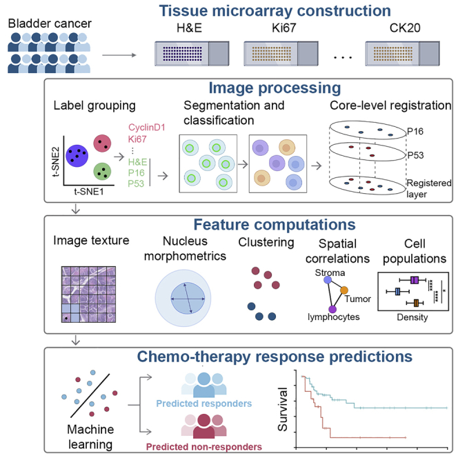
A computational framework was proposed to extract features from histology slides for patient stratification. The framework includes a central module and five submodules. First, TMAs were digitized and then imported to open-source image analysis software QuPath.¹⁶ In QuPath, the preprocessing step, including stain vector correction and core selection (see STAR Methods), was performed to prepare qualified cores for computations (Figure 2). First, image texture features were directly computed from raw H&E images. Next, core-level image registration and nuclei segmentation were performed to capture colocalized nuclei with respective labels. For each nucleus, centroid coordinate and a set of boundary points were both produced in this process. This information is input to compute nuclei morphology, clustering, and spatial correlational features. Then, a pathologist-supervised random tree-based classifier was trained to classify cells and nuclei into lymphocytes, cancer cells, and stromal cells, and their spatial distributions and correlations were quantified. The outputs from feature computations modules were combined to complete the feature matrix.

Figure 2.

Diagram of computational framework

The framework is initiated by tissue microarrays (TMAs) construction and image generation. Next, image preprocessing calibrates stain vectors for each TMA and then an area-variation-based criteria was adapted to select qualified cores for computational analysis. Afterward, image registration and segmentation were performed on all TMAs to obtain colocalized nuclei with respective labels. Nucleus centroid and a set of boundary points were the readouts in this process that are further loaded to feature computation modules to complete the feature matrix construction.

Image preprocessing

“TMA dearrayer” of QuPath identifies grid arrangements, and each grid represents a TMA core. The discovery cohort was represented on two TMAs from which multiple sections were taken that were stained for routine H&E along with multiple IHC. This thereby necessitated registration of the individual TMA core images for our analyses. Tissue area variations of the identified cores across different sections from the TMAs were calculated (see STAR Methods) and visualized as a heatmap (Figure 3A), wherein blue indicates low variability and red indicates high variability; the cross sign suggests at least one level for this core was marked as missing due to lack of tissue (such cores were discarded from downstream analysis). Area boxplot for a high variability (red in Figure 3B) suggested that area polarization and clustering may contribute to the high variations. As the spatial correlations between nuclei from different sections were computed in this study, image registration was required to colocalize different nuclei extracted from corresponding sections. Due to the sequential orientation of the sections taken from the TMAs, rather than a single reference image, we identified “adjacent” sections that were suitable for registration. To identify adjacent sections for robust image registration, we developed a three-step section grouping pipeline using t-distributed stochastic neighbor embedding (t-SNE) and k-means clustering algorithms (see STAR Methods). This resulted in the identification of groups of sections from the TMAs that exhibited high intra-group Spearman’s rank coefficient, thereby supporting the notion that they are suitable for registration (Figures 3C and S1–S4). Furthermore, TMA sections identified as adjacent visually have comparable local tissue landmarks that laid the basis for image registration (Figures 3D and 3E; see STAR Methods). Next, dice similarity coefficient (DSC) was employed to validate the registration accuracy.¹⁷ Results show that the average DSC scores reach over 0.95 for these TMA cores from the discovery cohort (Figure 3F), supporting the proposed registration pipeline. Outliers were mainly caused by the registration between incomplete sections of TMA cores. In the validation cohort, the extracted TMA core images from the H&E stains were subjected to color deconvolution to match the stain vector estimated of H&E from the validation cohort. There was only a single section of the validation cohort TMA; therefore, the registration pipeline described above was not needed.

Figure 3.

Image preprocessing pipeline

(A) For the TMAs of the discovery cohort, tissue areas were calculated over all stained sections and coefficient of variation (CoV) was computed. The CoV matrices were then visualized as heatmaps. Cross signs indicate at least one area value was missing due to insufficient tissue detected within the associated core. Such positions were discarded from further analysis. Scale bar, 200 μm.

(B) Area boxplot for a position (B-10, evaluable n = 8) with high variability suggests areas with specific stained sections were grouping with each other.

(C) t-SNE algorithm discovered TMA section adjacency groups for the section derived from the two TMAs that constituted the discovery cohort (evaluable labels for both set n = 9). Pearson correlation coefficients were calculated for within- versus across-section adjacency groups, with representative examples shown herein confirming the high correlation coefficient for within-adjacency group comparisons. Evaluable section pairs (n) = 96 for TMA set 1 and n = 121 for set 2.

(D) Similar local tissue landmarks shared by the cores with adjacent sections.

(E) Tissue boundaries are also registered using the transformation matrices generated during each image-level registration. Scale bar, 200 μm.

(F) DSC scores distribution for the discovery cohort. Though there are some outliers, the cohort achieved >0.95 mean DSC scores. Evaluable section pairs (n) = 801.

Image analysis and feature computations

Cores that passed preprocessing from both datasets were subject to image analysis and feature extraction. A deep learning-based algorithm StarDist¹⁸ was used to segment cells from section with nuclear staining (H&E, cyclin D1, Ki67, GATA3, P16, P53, and P63), and a classical watershed algorithm was used to segment cells from sections with membranous or cytoplasmic staining (CK5/6, CK20, and Her2Neu). Furthermore, 9 classifiers, each corresponding to a unique IHC stain, were trained to distinguish stain-positive nuclei. Because no classification was needed for H&E segmentations, the performance of segmentation algorithm itself was evaluated. But for IHC-stained sections, the segmentation and classification were treated as an integrated workflow such that the evaluation reflected their joint performance (see STAR Methods and supplemental information). The numerical estimates calculated in this process are deposited at Mendeley Data. In general, high precision and recall rates were achieved throughout all using cases. Moreover, a strong relation between the algorithmic detections and manual approach was observed (Spearman’s rank coefficient $r=$ 0.9966 for H&E and an average $r$ = 0.9728 for all processes with regard to IHCs). Linear regression results show that the slopes of fitted lines were always around 1 across all cases. Altogether, the segmentation algorithms and workflows show remarkable performances in segmenting nuclei and have strong agreements with human eyes and therefore validated for downstream computations. Parameters for algorithm setups were listed in Tables S1–S4.

In this study, computational features from qualified locations were extracted to formulate the final feature matrix. To calculate image texture features (see STAR Methods), cores with H&E staining were tiled into a series of 220 × 220 pixels rectangular tiles and transformed into grayscale images. Depending on the tissue size, the number of tiles per core ranges from 1 to 137 (median = 83) for the discovery cohort and from 5 to 178 (median = 136) for the validation cohort. For each 2D image matrix, 13 first-order statistics were calculated. Then, 12 distinct gray-level co-occurrence matrices (GLCMs) were created to comprehensively capture the texture variations. For each GLCM, 21 second-order statistics were computed (Figure 3A). In this part, 265 raw features are computed for each tile. To calculate the nucleus morphology features (see STAR Methods), a set of boundary points for each nucleus was recorded and 18 raw shape descriptors, such as areas and perimeters, were documented. To calculate the clustering features (see STAR Methods), Delaunay triangulations were generated for each core and a distance threshold was applied to identify clusters by removing long edges (Figure 4D). Then we measured 5 descriptors to characterize clustering features. Previous studies have shown the predictive value of cell/nucleus orientation entropy (COrE) in predicting recurrence in prostate cancer and non-small cell lung cancer.^19,20 We further extended the scope to predict treatment outcomes in MIBC. In this study, cell subgraphs were defined by each cluster, and cell and nucleus orientations were defined by calculating their first principal components. Two inputs jointly created a co-occurrence matrix to capture angle pairs that co-occur in each cluster (Figure 4C). We then computed 13 second-order statistics from each matrix.

Figure 4.

Image texture features, nucleus morphology, and clustering feature computations

(A) Image patches were generated from original H&E cores and then transformed to grayscale. For each grayscale pixel matrix, 12 different combinations of distance and angle were adapted to create 12 unique gray-level co-occurrence matrices (GLCMs). Features were then extracted from each GLCM. Scale bar, 20 μm.

(B) Shape descriptors were calculated for each segmented nucleus based on the boundary point set. Scale bar, 20 μm.

(C) First principal component was computed for each nucleus, and the angle of the component vector with horizontal direction was then derived to characterize the nucleus’s orientation.

(D) Delaunay triangulations and thresholding and cell/nucleus orientation entropy (COrE) map delineated in (C) jointly educated the render of the angle-pair co-occurrence matrix (APCM). Clustering and COrE features were computed for each cluster and APCM.

Spatial correlations were evaluated within groups with at least 2 IHC sections identified using t-SNE algorithm. For all IHC-stained sections within such groups, their associated nuclei coordinates were converted into point patterns and multi-type Ripley’s K function $K_{ij}\left(r\right)$ was used to compute spatial statistical features (see STAR Methods); note that the order of subscriptions reflects the computation order (i.e., $K_{ij}\left(r\right)$ computes the Ripley’s K from points of type i to points of type j). As $K_{ij}\left(r\right)$ and $K_{ji}\left(r\right)$ are not equal analytically, each pair of point patterns was evaluated twice with inverse input order (Figure 5A). Herein and referring back to Figure 3C, we computed 14 features for subset 1 and 24 features for subset 2, expressed in permutation formulas. The common features between two sets were selected for feature matrix.

Figure 5.

Spatial correlational and cell populational features computation

(A) Point patterns for a subset of labels from TMA subset 2 adjacency group 3. For each “adjacency” group identified using t-SNE algorithm, point patterns with each member marker (e.g., GATA3) were identified and spatial Ripley’s K function, $K\left(r\right)$, was computed. For each computation, $K\left(r\right)$ was evaluated at a series of distances until reaching a maximum distance of 20 μm. $K\left(r\right)$ produced theoretical and observation curves, and the area difference was calculated as spatial statistical features. Blue line, theoretical curve; red line, observation curve.

(B) Cell classification workflow: segmented nuclei data were subjected to cell classification and spatial dependency characterization using $K\left(r\right)$. Subscription: L (lymphocytes); C (cancer cells). Scale bar, 20 μm.

(C) Cell classification results. Cancer cells are generally large, immune cells are small and round, and stromal cells are usually elongated. The distributions of these cell types were then compared using boxplot and tri-plot: cancer cells prevailed other cell types over all cores from the discovery set. Scale bar, 20 μm. In TMA subset 1, evaluable cores (n) = 30 for responders and n = 36 for non-responders; in TMA subset 2, evaluable cores (n) = 24 for responders and n = 52 for non-responders. Comparisons for densities between cell types were assessed using Wilcoxon rank-sum test. ∗p < 0.05, ∗∗p < 0.01, ∗∗∗p < 0.001, and ∗∗∗∗p < 0.0001.

(D) $E_{SP}$was calculated to capture spatial heterogeneity. As a result, low $E_{SP}$ was found to associate with homogeneous regions, whereas high $E_{SP}$ scores associate with heterogeneous regions. Scale bar, 20 μm.

(E) Direct spatial proximity is a measure for every single cell by counting the number of cells of exterior types within the 20-μm range.

(F) Degree of colocalization (DoC) score was computed for each cell by comparing the cell density gradient of cells of its own type and target type. Cells with DoC scores larger than 0.847 were considered highly colocalized cells against target type.

To compute cell populational features, a pathologist-supervised, random tree-based classifier was trained to classify cells and nuclei from H&E slides into lymphocytes, cancer cells, and stromal cells (see STAR Methods). Then, we extracted following cell populational statistics from H&E tissue cores: first, $K_{ij}\left(r\right)$ again was applied to cell type pairs to compute spatial dependencies (Figures 5B and 5C). Next, a spatial adjusted Shannon’s entropy $E_{SP}$ was implemented to measure the diversity of cell species.²¹ The metric is spatially resolved as it incorporates the factor of distance. Theoretically, the increase of distance between the same type of points and the decrease of distance between different types of points cause the increase of entropy (see STAR Methods). As a result, low entropy scores are associated with regions where cell type dominancy occurs and high entropy scores are associated with diversified regions (Figure 5D). Evolved from spatial entropy analysis of different cell types, it is of interest to know whether they correlate with each other. For example, lymphocytes exhibit better anti-tumor immunity if they infiltrate into bulk tumors, but their effects are canceled when physical stromal barriers are presented nearby.²² A straightforward way to quantify the spatial correlation was measuring direct proximity for a single cell by identifying the number of nearest neighbors of each external type within 20 μm (Figure 5E). Spatial proximity captures the correlation between cells and their direct neighbors; however, the correlation patterns remain unknown. To address this challenge, we implemented the degree of colocalization (DoC) algorithm to quantitatively gauge the spatial correlations.²³ In this study, we focus on the correlation between three pairs of cell types: lymphocytes and cancer cells, lymphocytes and stromal cells, and stromal cells and cancer cells. For both cell types in each correlation pair, the DoC was computed and then assigned to every cell (see STAR Methods). DoC is a numerical score that bounded within [−1,1], suggesting anti-correlation to correlation. To identify highly colocalized cells, an empirical threshold was determined by shifting an existing point pattern left by 10 μm and then computing its DoC score with the parent point pattern. This approach results in 90% of total cells’ DoC being larger than 0.847, which was then defined as the threshold. For each pair, the number of highly colocalized cells and the distribution of DoC scores were measured as features (Figure 5F). Overall, 6 composition features, 6 spatial statistical features, 1 spatial entropy feature ($E_{sp}$ score), 6 direct spatial proximity features, and 12 raw DoC features were computed in this part. The above calculations were repeated for the validation cohort except spatial correlation features derived from the IHC stains, because only a single H&E-stained section was available for the validation cohort. All computed feature names were listed in Table S5.

Machine-learning models using computational pathology features improve accuracy in predicting neoadjuvant chemotherapy efficacy

Region-, cluster-, and cell-level features were first aggregated to core level (see STAR Methods). After aggregation, 1,187 features from 5 categories form the feature matrix used in these analyses: (1) 49 cell populational features; (2) 53 clustering features, derived from images of H&E staining; (3) 55 nucleus morphology features, derived from images of H&E staining; (4) 1,012 image texture features, derived from images of H&E staining; and (5) 18 spatial correlational features, derived from images of the various IHC stains we examined in this study. Of note, we observed strong variance at feature space across cores from the same patient (STAR Methods; Figure S5). To preserve such heterogeneity, we aggregated computational features and passed patient outcomes to core level such that predictions were made for each core. We then conducted 6 trials to evaluate the predictive power of various combinations of computational features. In the first trial, we trained four support vector machine (SVM) models with combinations of different kernels and types and a random forest (RF) model on demographic and clinicopathological (CP) features to establish a baseline. Due to the low dimensionality of CP features (Table S5), no feature selection was performed. SVM and RF models were trained and tested with 100× Monte Carlo cross-validation. For each run, CP feature matrix was randomly partitioned into training and internal validation set in ratio of 4:1. Using 16 CP features, our best SVM and RF models achieved mean accuracy (ACC) of 59.79% (SVM) and 54.21% (RF) and mean area under the receiver operating characteristic curve (AUC) of 0.54 (SVM) and 0.52 (RF). These values then served as the baseline against future trials. For trials 2–6, SVM and RF models were trained on 10 most relevant features selected using minimum-redundancy maximum relevance (mRMR) from each category to generate five standalone accuracies. Prediction results were summarized in Table S6.

The results showed single feature category could independently improve the mean performance up to 30.53% for ACC and 28.85% for AUC (RF model). In general, category 5 (features derived from IHC) confers the best independent performance in terms of both absolute ACC and AUC values and improvement rate and was universally observed across evaluated models. It is also noteworthy that variations of ACC were significantly reduced compared to the baseline, suggesting these features have better prediction stability across samples. We further measured the F1 score for each trial, and results indicate that the predictions were non-biasing. It is further of interest to know how different feature categories can be combined with each other and whether that will result in increased performance. We adapted 4 feature combination and analytical strategies: (I) 30 most relevant features that only rely on imaging of H&E slides (categories 2–4); (II) 40 most relevant features that rely on imaging of H&E slides and pathologist-derived measurements (categories 1–4); (III) 40 most relevant features derived solely from imaging of both H&E and IHC stains (categories 2–5); and (IV) 45 most relevant computational features over all possible categories (categories 1–5). We then focused on our best classifier (SVM with nu-classification and polynomial kernel) that reached a high mean ACC of 72.52% and AUC of 0.67 using all computational features. We first compare the AUC and ACC distribution after 100 runs of Monte Carlo cross-validation using one-way ANOVA, and we found both two metrics generate identical statistical inferences: all strategies perform significantly better than baseline in terms of ACC (Figure 6A) and AUC (see Figure S6). It is worth underscoring that analytical strategy I, which is based solely on the H&E images and does not require immunohistochemistry or clinical characterizations, was able to significantly improve the model performance compared to the baseline. We also observe some improvement in model performance using strategies III and IV, in which information from the various IHC stains were included in the model, suggesting that there could be a role in leveraging these types of biomarkers to further refine the predictive model. To validate our findings, we repeated the feature mining process on an external validation cohort, keeping the model fixed. Considering the validation cohort only contains H&E slides, spatial correlational features from the IHC stains examined in the discovery cohort were not computed; however, spatial features based on H&E were still included. Given that adding cell populational features and labels (category 1) did not significantly improve the model performance, we focused on validating the model using analytical strategy I, which is based on H&E-only derived features. Starting with a model using clinical and demographic features available across both cohorts (clinical T stage and age at operation), performance metrics were ACC = 59.31% ± 8.50%, AUC = 0.52 ± 0.06 for discovery cohort (training and cross-validation), and ACC = 59.49% ± 10.53% and AUC = 0.5 ± 0.11 for validation cohort (independent model testing). When adding H&E-derived features (feature selection performed with 30 most relevant features, forming strategy V), ACC and AUC metrics improved to an ACC of 69.17% ± 9.59% and AUC of 0.64 ± 0.09 across cross-validation in the discovery cohort and ACC = 65.82% and AUC = 0.61 in the external validation cohort. Adding H&E-derived features to the available baseline clinical and demographic features resulted in an increase performance of 16.62% and 23.08% for ACC and AUC, respectively. This supports the assertion that H&E-derived features could add predictive information in this clinical context above what is available in clinical and demographic data. Note, all model parameters for strategy V were trained using the discovery cohort and subsequently fixed prior to being applied to the validation cohort. In all cases, ACC was based on 0.5 threshold on model output (ranging from 0 to 1), in which we observed mean response rate of 64.64% for predicted responder as compared to the baseline response rate of 38.03% in the discovery cohort. A similar ability of the model from strategy V to enrich for responders was observed in the external validation cohort using the same 0.5 model threshold in which we observed a response rate of 64.71% for predicted responder as compared to the baseline response rate of 40.51% in the validation cohort.

Figure 6.

Classification results from machine learning models

(A) Comparison between ACC distributions after 100 runs of Monte Carlo cross-validation (CV) using different feature combination strategies. ACC for baseline and each strategy evaluated on discovery cohort is as follows: baseline (59.07% ± 11.8%); strategy I (65.38% ± 5.40%); strategy II (63.52% ± 5.40%); strategy III (70.34% ± 6.97%); and strategy IV (72.52% ± 6.99%). ACCs with strategy V (blue bar) on discovery cohort (69.17% ± 9.59%) and validation cohort (65.82% ± 10.46%) are shown, supporting the generalizability of the strategy V model. Data were presented in the format of mean ± SD over the distribution from Monto Carlo cross-validation in the discovery cohort and proportion ±95% confidence interval of that point estimate in the validation cohort. The ∗ designates that a subset of clinical and demographic features available across both discovery and validation cohorts (clinical T stage and age at operation) was used in strategy V. In discovery cohort, evaluable cores (n) = 54 for responders and n = 88 for non-responders; in validation cohort, n = 32 for responders and n = 47 for non-responders.

(B) Outputs from the best model: SVM with radial basis kernel and trained on all computational features. Among all features, 226 features have been selected at least once during 100 runs of CV. For those selected features, the top 10 most relevant features were identified based on their frequency and their associated feature categories are attached. The number of evaluable cores is consistent with (A).

(C) Comparison of enlisted feature distributions between responders and non-responders.

(D) Based on these distributions, 4 resistance-favored factors and 4 response-favored factors were hypothesized. While tumors in responders were more luminal-like and they tend to have rapid cancer proliferation rate, close spatial proximity, and more elongated cells, non-responders tend to have more diversified cell morphology, sparse nucleus spatial proximity, and a high degree of muscle-infiltrated tumor with lymphocyte-inflamed but immune-suppressed tumor microenvironment. One-way ANOVA test in (A) is performed by comparing group means; comparison in (C) is performed using two-tailed Welch two-sample t test. ∗p < 0.05, ∗∗p < 0.01, ∗∗∗p < 0.001, and ∗∗∗∗p < 0.0001.

We further explored the cooperativity of computational-derived and pathologist-measured features, in this case, the pathologist case/patient level estimate of the CD8-FoxP3. While all computational features were calculated from each core, CD8 and FoxP3 slides were not available, so we were unable to calculate core-level ratios. Alternatively, we directly used the patient-level ratio as a surrogate and then trained the SVM model. Importantly, the model attained a good accuracy of 72.62% ± 6.63% (AUC = 0.68 ± 0.07; F1 score = 0.80 ± 0.05). Although the value of CD8-FoxP3 ratio in predicting response to NAC is evident,¹⁰ it is still striking that the performance can be further improved only using the global ratio estimates. Unfortunately, we were not able to validate such finding, as IHC staining was not available for the external validation cohort. Nonetheless, such discovery corroborates the hypothesis that the immune system can modulate the response of bladder cancer to chemotherapy.²⁴

Machine-learning predictions may identify response-modulating factors in MIBC tumor microenvironment

To better understand the underlying pathological conditions that trigger the response to NAC, we identified top 10 ranked features that were derived from cross-validations of our best model with strategy IV. According to our study design, 100 runs of Monte Carlo cross-validation were performed, and for each run, the 45 most predictive features were selected for model training. Results show that, among the 100 feature selections, 226 features have been selected at least once (19.04% of total features). For those 226 features, top 10 features were chosen based on frequency (Figure 6B). Not surprisingly, spatial correlational feature was the dominant category, and no image feature was enlisted. By comparing their means over responders (Rs) and non-responders (NRs) (Figure 6C), we hypothesized two distinct patterns that may play a role in modulating the response to NAC (Figure 6D).

In responders (Rs), we observed high expression of CK20, which is associated with the luminal subtype of MIBC, a subtype which in some studies has been associated with response.²⁵ However, this association is somewhat tenuous, as there are also studies showing that the basal subtype is associated with this response.¹⁵ Interestingly, both Ki67 and P16 staining densities were significantly higher in responders. Increased Ki67 intensity is associated with increased cell proliferation, and overexpression of P16 is evidence of aberrant cell cycle regulation (usually due to defects in the Rb and/or P53 tumor suppressors).^26,27 This co-expression pattern of increased Ki67 and P16 that is linked to rapid cell proliferation is consistent with the general principle that more proliferative tumors should be more responsive to platinum-based chemotherapy. We also observed that the “area.of.triangle.min” score and “elongation.min” were found to be significantly high in responders, which indicates a tight spatial and high ratio of elongated cells.

In NR, “min.diameter.CoV” and “MOI_CoV,” which measures the variations of nuclei’s minimum diameter and moment of inertia, were high in NR. High CoVs suggest nuclei shapes in NR’s tumor sites were more diverse; “COrE_IDM_mean” was also found to be high in NR, indicating cell orientations in NR tumors were more chaotic; the low CD8+/FoxP3+ ratio as previously described indicates that the present lymphocytes are mainly regulatory T cells (Treg cells); and in addition, low “DoC_TS_max” and high “DoC_SL_mean” indicate that the tumor infiltration of lymphocytes was impeded by stromal barrier. Taken together, the immuno-suppression effect of Treg cells and severe stromal burden may hypothetically result in an impaired anti-tumor immunity that favors the resistance to NAC. However, one important caveat is some selected features did not attain statistical significance among R and NR, demonstrating that patterns shall be interpreted with caution and require further validations.

Machine learning predictions stratify patients into good and poor survival group

We further tested the potential of our best model in patient survival stratifications. For each run of Monte Carlo cross-validation, predicted probabilities of being Rs of each selected core in testing set were recorded. Next, predicted outcome label was assigned to each core using a series of cutoff thresholds of model outputs ranging from 0.1 to 0.9. Patient-specific survival data were assigned to each core to keep the analytical logic consistent. A significant stratification (log rank p < 0.01) of overall survival was observed with a model threshold of 0.25 in the discovery cohort, wherein predicted responders exhibited improved overall survival (Figure 7). Survival data were not available for the validation cohort; however, the findings in the discovery cohort are consistent with the well-established understanding that MIBC patients who respond to NAC exhibit improved clinical outcomes.

Figure 7.

Patient survival stratification using predicted outcomes

(A) Patient stratification strategy. Probabilities of being responders for each core were averaged over cross-validation in the discovery cohort and compared to a series of thresholds ranging from 0.1 to 0.9. Patients that were predicted responders were labeled as low-risk group, and conversely, predicted non-responders were labeled as high-risk group.

(B) Kaplan-Meier curve for the optimized split (threshold = 0.25) based on cross-validation in the discovery cohort. p value was computed using log rank test.

Discussion

In this study, we developed predictive models of cisplatin-based NAC in MIBC based on nucleus morphology and tissue architecture, including imaging from IHC staining of various salient proteins in the context of MIBC. We analyzed H&E- and IHC-stained section from TMAs collected from the discovery cohort and subsequently tested in an independent validation cohort (H&E only), all of which were composed of comparable MIBC patients treated with NAC.

In this study, we were able to, in part, perform some degree of data augmentation (in attempt to increase the relative number of data points) by formulating the classification task at the level of distinct regions of tissue (i.e., each core in the TMA) rather that at the patient level, which is usually sampled multiple times on a TMA via multiple cores. TMA cores represent regional sampling of a given specimen (usually ~1 mm), and as such, our workflow can be readily generalized to sampling of different regions from whole slide imaging as needed. Further, analysis of core-level data preserves the intra-tumoral heterogeneity coming out of the patient, which makes the proposed models less sensitive to the location where the cores were taken from and allows a flexible design of TMA. Future work will be required to extend these approaches to aggregate sampling from multiple regions of a tumor into a single measure for that sample/patient in order to be best utilized clinically; unfortunately, the size of the discovery and validation cohorts in terms of patient numbers did not support this approach analytically.

Previous studies have shown that image features and machine learning techniques can discern subtle differences that are not readily noticeable to pathologists between tissues from patients with different disease subtypes, cancer grades, and survival;28, 29, 30, 31 here, we further extend the scope to predict response to NAC in MIBC. Spatial heterogeneity is a hallmark of cancer, and features of the tumor microenvironment (TME) may drive tumor responses to specific therapies.³² Profiling of TME can provide critical insight into such heterogeneity, which motivated us to develop predictive models by quantitative characterization of TME.³³ Specifically, spatial heterogeneity is reflected by alternations in various levels, ranging from single-cell to tissue architecture.^34,35 Therefore, we carefully designed our feature matrix in a multi-level manner and hypothesized that such characterization could capture the hidden variations.

The framework involved computational derivation of image-based features that quantitatively characterized tissue regions and the cells contained therein covering 5 different classes: image texture; nucleus morphology; clustering; spatial correlations; and cell population. The predictive power of each category was tested by identifying a subset of features that was most relevant to NAC treatment response jointly with SVM and RF models in cross-validations. In this study, all engineered features were carefully crafted and care was taken to explicitly allow for model explainability. In Figure 6A, we presented the 10 most predictive features from our best classifier, and distributions across Rs and NRs were gauged. Specifically, non-responsive tumors tended to associate with more diversified cell morphology and orientation, stromal burden, and low CD8/FoxP3 ratio, while responsive tumors tended to associate with rapid proliferation, close spatial proximity, more elongated cells, and features of a luminal MIBC subtype (CK20 staining). The biological and mechanistic relevance of these associations would have to be tested experimentally.

Our results suggest that image features could enhanced prediction accuracy for Rs and NRs to NAC in MIBC and provide potentially more stable performance in comparison to a baseline model of only conventional clinicopathologic variables. We explored potential synergistic effects with different combinations of feature categories and observed that the addition of imaging-derived features from the H&E-derived features to standard clinical and demographic information in this context (strategy V) is able to improve performance from baseline to achieve cross-validation estimated accuracy of 69.17% in the discovery cohort based on 0.5 model threshold, in which we observe an enriched response rate of 64.64% in predicted responders relative to the baseline response rate of 38.03% in the discovery cohort. Importantly, in an independent validation cohort, the applicable model trained on the discovery cohort is able to achieve comparable accuracy of 65.82% and enriched response rates of 64.71% in predicted responders as compared to the baseline response rate of 40.51% in this cohort. Hence, a similar ability of the model to enrich for responders is observed across discovery and validation cohort, attesting to the generalizability of the approach. These promising results, however, are based on relatively smaller sized cohorts and will need additional validation with larger sized cohorts in addition to the need to aggregate information from multiple sampling points from a given sample/patient. Consistent with the previous reports from this cohort, the CD8/FoxP3 ratio metric derived from human interpretation is a significant predictor of response (mean ACC = 72.62%; mean AUC = 0.68). However, the variability of these measures in cross-validation of the discovery cohort overlapped the performance estimates of models that use H&E only (i.e., no IHC-stained sections). Additionally, only an H&E-stained section from the validation cohort was available for assessment of generalizability. Taken together, the results from the discovery cohort suggest that the inclusion of the salient IHC staining of key tumor and immunological biomarkers will increase performance, but based on the limited size of this dataset, we cannot establish this at this point.

In summary, we explored the predictive power of multi-scale computational features extracted from histology and immunohistology images of response to NAC in treating MIBC. The features attained from the process pipeline are carefully hand crafted to ensure biologically interpretability and reproducibility. To the best of our knowledge, this presents a pioneering work in utilizing image features for such stratification. Although no population-level inference will be made at this point, our workflow is fully automated and reproducible for additional evaluation. Importantly, our results reveal that routine H&E slides could yield response prediction power. Given that H&E staining is ubiquitously available, our study could potentially advance the treatment for MIBC patients in a fast and low-cost manner.

Limitations of the study

There are several limitations to this study worth mentioning. Although data augmentation was implemented and performance was characterized in strict cross-validation and independent external cohort, the sample size was still small and prevented us from making population-level inference. Importantly, the IHC-based models cannot be fully validated due to the lack of IHC staining in the external validation cohort. In this study, proteins were stained on consecutive cores of tumor biopsy; therefore, registration was required to measure their spatial correlations. However, registration cannot fully align the tissue images in the context of serial section from tissue; hence, the derived point patterns do not completely reflect real nucleus distributions across all IHC stains. Multiplexing methods, on the contrary, enable simultaneous profiling of multiple protein markers; in this case, location mismatches, tissue folds, and z axis differences are substantially eliminated. Though predictions and inferences have been occasionally made at core level,^36,37 the proposed model with selected features should be further assessed by larger cohort at patient level to render clinical application values. In addition, manually engineering features is viable when handling low-dimensional dataset; however, in future studies, we intend to increase the region of interest (ROI) resolution from tumor microenvironment to cell niche, which would exponentiate the computational cost. In this context, (1) handcrafting features would be low efficient and (2) extracted features are hardly interpretable due to high texture subtlety. The aforementioned issue can be alleviated by incorporating artificial intelligence, such as convolutional neural networks, which could facilitate the feature mining in an end-to-end manner. This enables feature engineering without discipline expertise and hardcore handcrafting.

STAR★Methods

Key resources table

REAGENT or RESOURCE	SOURCE	IDENTIFIER
Antibodies
Mouse monoclonal anti-P16	Roche/Ventana	Cat#705-4793; RRID: AB_2833232
Mouse monoclonal anti-P53	Roche/Ventana	Cat#760-2542; RRID: N/A
Rabbit monoclonal anti-Ki67	Roche/Ventana	Cat#790-4286; RRID: AB_2631262
Mouse monoclonal anti-CK5/6	Roche/Ventana	Cat#790-4554; RRID: AB_2861320
Rabbit monoclonal anti-Her2	Roche/Ventana	Cat#790-2991; RRID: AB_2335975
Mouse monoclonal anti-P63	Biocare Medical	Cat#PM163AA; RRID: AB_10582857
Mouse monoclonal anti-GATA3	Biocare Medical	Cat#CM405B; RRID: N/A
Mouse monoclonal anti-CK20	Cell Marque	Cat#320M-18; RRID: AB_1158255
Rabbit monoclonal anti-CyclinD1	Roche/Ventana	Cat#790-4508; RRID: AB_2335988
Biological samples
H&E and IHC tissue microarrays - Discovery cohort	Johns Hopkins University School of Medicine	N/A
H&E tissue microarray - Validation cohort	University Hospital Bern	N/A
Deposited data
GitHub	Raw features	https://github.com/popellab/MIBC-Predictive-models/tree/Code
Mendeley Data	Performance evaluations of segmentation and classification algorithms	https://doi.org/10.17632/v7xh2m76tw.1
Software and algorithms
QuPath (version 0.2.0-m12)	Bankhead et al.16	https://qupath.github.io/
MATLAB (verson 2020a)	MathWorks	https://www.mathworks.com/products/matlab.html
R (version 3.5.3)	CRAN	https://www.r-project.org/
RStudio desktop (version 1.4)	RStudio	https://www.rstudio.com/
Python (version 3.8)	Python Software Foundation	https://www.python.org/
Pycharm Python IDE (version 2020.3.3)	JetBrains	https://www.jetbrains.com/pycharm/
StarDist	Schmidt et al.18	https://github.com/stardist/stardist
https://github.com/popellab/MIBC-Predictive-models/tree/Code	Analysis code	N/A
Prism (version 9.0.0)	GraphPad Software	https://www.graphpad.com/scientific-software/prism/
BioRender	BioRender	https://biorender.com/
Adobe Photoshop CC (2020)	Adobe	https://www.adobe.com/

Resource availability

Lead contact

Requests for additional information, resources and reagents should be directed to the lead contact, Haoyang Mi (hmi1@jhmi.edu)

Materials availability

This study did not generate new unique reagents.

Experimental model and subject details

For discovery cohort, we queried the Johns Hopkins Hospital (JHH) Institutional Review Board approved bladder cancer database to include 73 patients who received cNAC followed by open RC between 2000 and 2013. Patients with unknown follow-up, cause of death, or documentation of inadequate cNAC dosing (receive less than 3 cycles of cNAC regimens) were excluded from the cNAC subset described above. Here, dose reduction was defined as a reduction in either gemcitabine or cisplatin dose owing to patient intolerance as defined in the original publication on this cohort¹². For the purposes of this study, all pre-treatment biopsy (TUR) specimens meeting criteria were examined based on imaging of hematoxylin and eosin or the designated immunohistochemical staining of these tissues. For the external validation cohort, 56 patients with MIBC from University Hospital Bern were selected, whose characteristics were comparable to the discovery cohort. IHC staining and antibody details were provided in supplemental information. Please refer to our previous studies for clinicopathological and demographic features of the discovery cohort10, 11, 12 and validation cohort13, 14, 15. The studies involving human participants were reviewed and approved by the clinical research ethnics board of each institution. Written informed consent for participation was not required for this study in accordance with the national legislation and the institutional requirements.

Method details

Core selection

As we aimed to extract cancer-associated features for patient stratification, only cores from the tumor site were considered in this study. Furthermore, we observed some cores were subjected to severe tissue loss due to the sectioning and staining. Such cores contain less or no histology information and therefore should not be included in the downstream computational analysis. Given the dimension of each TMA, we first used the ‘TMA dearrayer’ algorithm in QuPath to identify cores and grid arrangement. Each core would be assigned an identifier using a combination of letter and number (e.g., A-1) to suggest its column and row position. And the algorithm would set a core as missing if the detected tissue below the density threshold. To ensure the integrity of materials, we removed locations that have at least one missing core.

Core registration

A 3-step pipeline was proposed to group markers for registration. To start, a pixel classifier was trained to capture tissue boundaries and associated tissue areas for the core to quantify the tissue variations. For each dataset, these procedures were repeated for all selected locations across 10 sections (H&E, Ki67, p53, etc) and the area variations for each location can be computed using coefficient of variation (CoV), defined as:

$$CoV=\frac{\sigma }{\mu }$$

where $\sigma$ and $\mu$ denote the standard deviation and mean of areas, respectively. Let us define the number of selected locations as $n$. Suppose ten markers were defined as variable ν_x, where x = 1, 2, …, 10; then the tissue area of variable ν_x at location n as A_{x, n}. Such that:

$$v_1=\{A_{1,1},A_{\mathrm{1,2}},A_{\mathrm{1,3}},\dots ,A_{1,n}\}$$

$$v_2=\{A_{2,1},A_{\mathrm{2,2}},A_{\mathrm{2,3}},\dots ,A_{2,n}\}$$

$$v_{10}=\{A_{10,1},A_{\mathrm{10,2}},A_{\mathrm{10,3}},\dots ,A_{10,n}\}$$

With each $v_x$ is an n-dimensional object, the third step was applying t-distributed stochastic neighbor embedding (t-SNE) algorithm to map each object to two-dimensional space and ‘kmeans’ clustering algorithm was performed to detect groups with similar objects. Hence, the associated markers within each group were considered as adjacent markers to each other and were eligible for registration. For each group, one member was selected as the reference and should be kept consistent across each location. The registration was performed using the MATLAB toolbox ‘Registration Estimator’. Also, each round of registration will generate a transformation matrix that can be used to register coordinates.

To validate the pipeline, the Pearson correlation coefficient between each pair of $v_x$ from the same cluster and among different clusters were computed. High intra-cluster coefficients and low inter-cluster coefficients suggested successful grouping. For each location, the boundaries of reference and moving cores were extracted as polygons in coordinates format. Then, polygons from moving cores were registered using corresponding transformation matrices. Next, Dice Similarity Coefficients (DSC) were measured for each pair of reference-moving polygon. DSC is a spatial overlap index and the value ranges from 0, indicating no overlap between two polygons, to 1, indicating complete overlap. Therefore, high overall DSCs across all pairs suggested successful registration. For simplicity, only positions that all associated cores were intact (only one tissue piece) were included to evaluate the registration accuracy in this study. Values of parameters to set up the MATLAB registration algorithm were listed in supplement Table S1.

Nucleus segmentation and classification

A previously described workflow was adapted³³. In brief, color deconvolution was performed to correct the stain vectors of each TMA slide. Then, a deep learning-based method called ‘StarDist’ was used to detect nucleus-stained cells¹⁸. A tutorial that describes how to implement StarDist directly within QuPath is provided here: https://qupath.readthedocs.io/en/latest/docs/advanced/stardist.html. Also, a built-in unsupervised watershed algorithm within QuPath was used to detect membrane-stained cells. Afterward, nine Random Tree classifiers, each for a single IHC TMA, were trained to detect positive nuclei. Parameter values to set up the segmentation and cell classification algorithms were listed in Tables S2–S4.

Performance evaluation of segmentation and classification algorithms

The evaluation process was carried out by randomly selecting 200 sub-regions (100 from each of the TMAs of the discovery) with a size of 100 × 100μm from all qualified cores. Then, nuclei were counted using both algorithm and manual approach. After all counts were recorded for 200 sub-regions, the following statistics were summarized: the number of nuclei that detected both manually and by the algorithm/workflow (true positive, TP); the number of nuclei detected manually but were missed by the algorithm/workflow (false negative, FN); the number of nuclei detected by the algorithm/workflow but rejected by manual approach (false positive, FP). Based on these statistics, the following metrics were calculated to evaluate the performance of the algorithm/workflow:

$$R=\frac{TP}{TP+FN}$$

$$P=\frac{TP}{TP+FP}$$

$$s{e}_R=\sqrt{\frac{R\cdot (1-R)}{TP+FN}}$$

$$s{e}_P=\sqrt{\frac{P\cdot (1-P)}{TP+FP}}$$

whereas $R$ denotes Recall rate (Sensitivity), and $P$ denotes Precision (1 – false discovery rate); $s{e}_R$ and $s{e}_P$ denotes their standard error of mean, respectively. In addition, the correlation between algorithmic results and manual approach results were evaluated calculating the Spearman’s rank coefficient.

Computation of image texture features

Image texture features were calculated from gray-level co-occurrence matrices (GLCMs) extracted from H&E slides. First, each qualified H&E core was split into multiple tiles of 220 $\times$ 220 pixels and trimmed to tissue boundaries to exclude backgrounds. As GLCM requires input tiles image to be rectangles, irregular-shaped tiles were removed from further computations. Next, all rectangular tile images were converted to grayscale images. At this point, 13 first-order statistics were computed to characterize the grayscale image. To further capture the texture feature defined by the input image, 12 GLCMs were created based on 12 spatial pixel relationships of varying distances ($d$ = 1, 3, 5) and directions ($\theta =0°,45°,90°,135°$). Next, 21 s-order statistics (features) that describe the pixel distributions in each GLCM were derived. The GLCM features were calculated using the function ‘glcm’ from R package radiomics. Complete feature names were listed in Table S5.

Computation of nucleus morphology

QuPath segmentation algorithms converted a single nucleus boundary to a point collection, which can be mapped to form a polygon that mimics the corresponding nucleus object. For each polygon, 18 nucleus morphology descriptors were computed. R packages sf and smoothr were used to interpolate point sets of nucleus boundary where necessary. Complete nucleus morphometrics names were listed in Table S5.

Computation of clustering features

As nuclei, especially cancer nuclei, are often densely exist in tissue cores, density-based clustering algorithms like DBSCAN and HDBSCAN usually underperform in such cases. Hence, a spatial distance-resolved clustering workflow was used for clustering identification. Such workflow has been validated in previous studies and shows better performance in feature mining from tissue microarray images. For each qualified H&E core, nuclei were used as nodes to create Delaunay triangulation network and edges were used to model the spatial interaction between two connected nodes (nucleus). Next, an empirical distance threshold was applied to remove long edges which indicate a low probability of spatial engagement. Next, clusters were defined as maximal connected components of the network with at least 30 nodes. Considering the cut of tissues is a deterministic factor of cluster shapes in TMA cores, we only extracted non-morphometric features, such as the number of triangles, from each cluster. Next, the clustering information and nucleus orientations can be merged to calculate the cell/nucleus orientation entropy (COrE) features. In brief, statistical features were derived from nucleus orientation angle co-occurrence matrices created for each cluster. Detailed methodology was described by Lee et al.¹⁹. The Delaunay triangulation was generated using functions ‘tri.mesh’ and ‘triangles’ from R package tripack; maximum connected components were detected using function ‘components’ from R package igraph. Complete clustering feature names were listed in Table S5.

Computation of spatial correlational features

Centroid coordinates of nuclei were transformed to point patterns. For each location, multitype Ripley’s K function was computed to count the observed and theoretical number of nuclei of type $i$ (e.g., CyclinD1) within 20 μm of nuclei of type $j$ (e.g., Ki67), where $i$ and $j$ were adjacent labels. $K\left(r\right)$ was evaluated at a series of consecutive distances until reaches maximum evaluation distance $d$. As a result, two curves were created and the area difference was calculated to characterize the dependence between the points of type $i$ and $j$. In this study, we assume the density of a point pattern is homogeneous over the tissue core as the region was small. Hence, $K\left(r\right)$ can be computed using the function ‘Kcross’ from R package spatstat. Complete clustering feature names were listed in Table S5.

Computation of cell population features

101 cells/nuclei were randomly selected from 20 H&E cores from TMA subset 1 and then annotated into 3 classes: lymphocytes (L), cancer cells (C), and stromal cells (S), by pathologist ASB based on their morphology. Specifically, 36 lymphocytes, 9 stromal cells, and 56 cancer cells were annotated. Next, a random tree classifier was trained and then tested on cells in another 20 cores from TMA subset 2. Afterward, 157 cells with predicted types were censored by ASB, and corrections were made accordingly to fine-tuning the classifier.

The classifier then assigned types to all other nuclei. For a nucleus set $S_k=\left\{V\right\}$, where$i$ represents the nucleus type $k\in \{L,C,S\}$, and $V$ represents the set of the associated 2D nuclear centroid ${\gamma }_x,{\gamma }_y\in V$, $\gamma \in \{\mathrm{1,2},\dots ,n\}$. Next, direct spatial proximity was computed. For each nucleus set $S_k$, the number of all immediate neighbors from other sets were computed using the formula:

$$N_j\left(\gamma \right)=\left\{\dim \left(\beta \right):d\left(\beta ,\gamma \right)\le d_t,\forall \gamma \in S_i,\forall \beta \in S_j\right\}$$

where $j\in V\cap \left(j\ne i\right)$; $d(\beta ,\gamma )$ represents the Euclidean distance between nucleus $\gamma$ of set $i$ and nucleus $\beta$ of set $j$. $d_t$ represents an empirical proximity threshold. To compute the spatial dependency, multiple $K\left(r\right)$ was evaluated for each cell type pair. The spatial Shannon’s entropy is defined as:

$$E_{SP}=-\sum _{i=1}^n\frac{d_i^{int}}{d_i^{ext}}{p}_i{\log }_2{p}_i$$

where ${\text{d}}_i^{\text{int}}$ represents the average Euclidean distance between all points from set $i$; ${\text{d}}_i^{\text{ext}}$ represents the average Euclidean distance between all points from set $i$ and the points of all other sets; $p_i$ is the percentage of type $i$ within the core.

To compute the degree of colocalization (DoC) for a given cell type pair, a series of circles with increasing radius were generated centered at each nucleus of from set $i$. Then for each circle, densities of type $i$ nucleus and type $j$ nucleus were calculated and Spearman’s rank coefficient ${\rho }_{ij}$ was measured between two density gradients. Next, each coefficient was weighted to a DoC score using the equation:

$$D_i={\rho }_{ij}\cdot e^{(-\frac{N_{ij}}{R_{max}})}$$

where $N_{ij}$ is the distance of the current point to its nearest neighbor of type $j$. $R_{max}$ is the maximum search radius.

Nucleus-nucleus Euclidean distance was calculated using function ‘nn2′ from R package flexclust; A C++ implemented k-dimensional tree search (cKDTree) algorithm from Python library Scipy³⁸ was used to accelerate searching of nearest neighbors; Spearman’s rank coefficient was calculated using function ‘spearmanr’ also from ‘Scipy’. Complete clustering feature names were listed in Table S5.

Feature aggregations

Core-level feature is the unit for feature matrix construction. However, the majority of features computed using the aforementioned procedures were tile-level (image texture features) and cell/nucleus level features (shape descriptors). Therefore, data aggregation was needed to unify all features to the same level. In this study, four metrics: maximum, minimum, mean, and coefficient of variation (CoV) were computed for all non-core level features. Each aggregated feature corresponded to four core-level features, and suffixes ‘_mean’, ‘_max’, ‘_min’, and ‘CoV’ (or ‘Std’ if the data vector could contain negative values) were assigned to each core-level feature indicating the aggregation metric.

Assessment of inter-core heterogeneity in feature space

For both discovery and external validation cohort, patients with at least two cores were subject to heterogeneity analysis. For each patient, Pearson’s correlation coefficient $\rho$, range from −1 to 1, were computed for each pair of scaled core-level feature vectors. High $\rho$ indicates two feature vectors were correlated therefore confer low inter-core variance; conversely low $\rho$ indicates heterogeneity across cores at feature space.

Feature selection

The feature matrix was created by combining all features so that each row represented a sample (core) and each column represented a feature. Depends on the status of each patient, either 0 (responder) or 1 (non-responder) was assigned to associated cores as the target variable. To avoid data overfitting due to the high dimensionality of the feature matrix but relatively small sample size, minimum redundancy maximum relevance (mRMR) algorithm was used to reduce the feature dimensions. mRMR can find a subset of most discriminative features that jointly maximizing the correlation to the target variable while minimizing redundancy within themselves. Feature selection was only performed to the training set and different numbers of predictive features were selected (depends on the scale of feature pool).

Classifier construction and evaluation

Support vector machine (SVM) with combinations of two types (C-classification and nu-classification) and two kernels (radial and polynomial) and random forest (RF) models were implemented in this study. A 100-fold Monte Carlo cross-validation method was used to evaluate classifiers. For each fold, the feature matrix was split into a training set and internal validation set with a ratio of 4:1. Depending on the feature assembly strategy, 10 - 45 most predictive features were identified by mRMR. The model accuracy (ACC), which defined as:

$$ACC=\frac{Numberofcorrectpredictions}{Totalnumberofpredicitons}$$

area under the receiver operating characteristic curve (AUC), and F1 score reached during the cross-validation were labeled to describe the performance for the fold. After the cross-validation, all recorded ACC, AUC, and F1 score were averaged to characterize the overall predictive value of features. For external validation, features that were common across both discovery and validation cohort (i.e., feature categories 2, 3, 4 in conjunction with clinical and demographic features) were used for feature selections and the entire discovery cohort were used for training. Same model evaluation metrics: ACC, AUC, and F1 score were computed on the external validation cohort. For discovery cohort, evaluations metrics with mean and standard deviations were reported. For validation cohort, standard deviations were incomputable since the model output is a single number. In this case, 95% confidence interval was computed. mRMR was performed using function ‘mRMR.ensemble’ in R package mRMRe; SVM classifier was trained using function ‘svm’ in R package e1071; RF classifier was trained using function ‘randomForest’ in R package randomForest.

Quantification and statistical analysis

One-way ANOVA test and comparisons between the means of two populations were done using either a Welch two-sample t test or Wilcoxon rank-sum test using GraphPad Software. We performed the log-rank test to compare the survival times between predicted low risk versus high risk group using ‘survdiff’ function in R package survival. Kaplan-Meier curve and risk tables were generated using ‘ggsurvplot’ function in R package survminer.

Published: August 27, 2021

Data and code availability

The datasets generated or analyzed during this work are made publicly available at GitHub: https://github.com/popellab/MIBC-Predictive-models/tree/features. Raw pathology specimen slides for both discovery and external validation cohort were available from the corresponding author upon reasonable requests. The codes for computational methods are made publicly available at GitHub: https://github.com/popellab/MIBC-Predictive-models/tree/Code. Performance evaluations of segmentation and classification algorithms are deposited at Mendeley Data: https://doi.org/10.17632/v7xh2m76tw.1.

References

- 1.Howlader N., Noone A., Krapcho M., Miller D., Bishop K., Kosary C., Yu M., Ruhl J., Tatalovich Z., Mariotto A. National Cancer Institute; 2017. SEER Cancer Statistics Review, 1975-2014; pp. 1–12. [Google Scholar]
- 2.Ghosh M., Brancato S.J., Agarwal P.K., Apolo A.B. Targeted therapies in urothelial carcinoma. Curr. Opin. Oncol. 2014;26:305–320. doi: 10.1097/CCO.0000000000000064. [DOI] [PMC free article] [PubMed] [Google Scholar]
- 3.Grossman H.B., Natale R.B., Tangen C.M., Speights V.O., Vogelzang N.J., Trump D.L., deVere White R.W., Sarosdy M.F., Wood D.P., Jr., Raghavan D., Crawford E.D. Neoadjuvant chemotherapy plus cystectomy compared with cystectomy alone for locally advanced bladder cancer. N. Engl. J. Med. 2003;349:859–866. doi: 10.1056/NEJMoa022148. [DOI] [PubMed] [Google Scholar]
- 4.Motterle G., Andrews J.R., Morlacco A., Karnes R.J. Predicting response to neoadjuvant chemotherapy in bladder cancer. Eur. Urol. Focus. 2020;6:642–649. doi: 10.1016/j.euf.2019.10.016. [DOI] [PubMed] [Google Scholar]
- 5.Vale C., Advanced Bladder Cancer (ABC) Meta-analysis Collaboration Neoadjuvant chemotherapy in invasive bladder cancer: update of a systematic review and meta-analysis of individual patient data advanced bladder cancer (ABC) meta-analysis collaboration. Eur. Urol. 2005;48:202–205. doi: 10.1016/j.eururo.2005.04.006. discussion 205–206. [DOI] [PubMed] [Google Scholar]
- 6.Guo C.C., Bondaruk J., Yao H., Wang Z., Zhang L., Lee S., Lee J.-G., Cogdell D., Zhang M., Yang G. Assessment of luminal and basal phenotypes in bladder cancer. Sci. Rep. 2020;10:9743. doi: 10.1038/s41598-020-66747-7. [DOI] [PMC free article] [PubMed] [Google Scholar]
- 7.Tse J., Ghandour R., Singla N., Lotan Y. Molecular predictors of complete response following neoadjuvant chemotherapy in urothelial carcinoma of the bladder and upper tracts. Int. J. Mol. Sci. 2019;20:793. doi: 10.3390/ijms20040793. [DOI] [PMC free article] [PubMed] [Google Scholar]
- 8.Litjens G., Bandi P., Ehteshami Bejnordi B., Geessink O., Balkenhol M., Bult P., Halilovic A., Hermsen M., van de Loo R., Vogels R. 1399 H&E-stained sentinel lymph node sections of breast cancer patients: the CAMELYON dataset. Gigascience. 2018;7:giy065. doi: 10.1093/gigascience/giy065. [DOI] [PMC free article] [PubMed] [Google Scholar]
- 9.Campanella G., Hanna M.G., Geneslaw L., Miraflor A., Werneck Krauss Silva V., Busam K.J., Brogi E., Reuter V.E., Klimstra D.S., Fuchs T.J. Clinical-grade computational pathology using weakly supervised deep learning on whole slide images. Nat. Med. 2019;25:1301–1309. doi: 10.1038/s41591-019-0508-1. [DOI] [PMC free article] [PubMed] [Google Scholar]
- 10.Baras A.S., Drake C., Liu J.-J., Gandhi N., Kates M., Hoque M.O., Meeker A., Hahn N., Taube J.M., Schoenberg M.P. The ratio of CD8 to Treg tumor-infiltrating lymphocytes is associated with response to cisplatin-based neoadjuvant chemotherapy in patients with muscle invasive urothelial carcinoma of the bladder. OncoImmunology. 2016;5:e1134412. doi: 10.1080/2162402X.2015.1134412. [DOI] [PMC free article] [PubMed] [Google Scholar]
- 11.Baras A.S., Gandhi N., Munari E., Faraj S., Shultz L., Marchionni L., Schoenberg M., Hahn N., Hoque M.O., Berman D. Identification and validation of protein biomarkers of response to neoadjuvant platinum chemotherapy in muscle invasive urothelial carcinoma. PLoS ONE. 2015;10:e0131245. doi: 10.1371/journal.pone.0131245. [DOI] [PMC free article] [PubMed] [Google Scholar]
- 12.Gandhi N.M., Baras A., Munari E., Faraj S., Reis L.O., Liu J.-J., Kates M., Hoque M.O., Berman D., Hahn N.M. Gemcitabine and cisplatin neoadjuvant chemotherapy for muscle-invasive urothelial carcinoma: predicting response and assessing outcomes. Urol. Oncol. 2015;33:204.e1–204.e7. doi: 10.1016/j.urolonc.2015.02.011. [DOI] [PMC free article] [PubMed] [Google Scholar]
- 13.Kiss B., Wyatt A.W., Douglas J., Skuginna V., Mo F., Anderson S., Rotzer D., Fleischmann A., Genitsch V., Hayashi T. Her2 alterations in muscle-invasive bladder cancer: patient selection beyond protein expression for targeted therapy. Sci. Rep. 2017;7:42713. doi: 10.1038/srep42713. [DOI] [PMC free article] [PubMed] [Google Scholar]
- 14.Fleischmann A., Thalmann G.N., Perren A., Seiler R. Tumor regression grade of urothelial bladder cancer after neoadjuvant chemotherapy: a novel and successful strategy to predict survival. Am. J. Surg. Pathol. 2014;38:325–332. doi: 10.1097/PAS.0000000000000142. [DOI] [PubMed] [Google Scholar]
- 15.Seiler R., Ashab H.A.D., Erho N., van Rhijn B.W.G., Winters B., Douglas J., Van Kessel K.E., Fransen van de Putte E.E., Sommerlad M., Wang N.Q. Impact of molecular subtypes in muscle-invasive bladder cancer on predicting response and survival after neoadjuvant chemotherapy. Eur. Urol. 2017;72:544–554. doi: 10.1016/j.eururo.2017.03.030. [DOI] [PubMed] [Google Scholar]
- 16.Bankhead P., Loughrey M.B., Fernández J.A., Dombrowski Y., McArt D.G., Dunne P.D., McQuaid S., Gray R.T., Murray L.J., Coleman H.G. QuPath: open source software for digital pathology image analysis. Sci. Rep. 2017;7:16878. doi: 10.1038/s41598-017-17204-5. [DOI] [PMC free article] [PubMed] [Google Scholar]
- 17.Guy C.L., Weiss E., Che S., Jan N., Zhao S., Rosu-Bubulac M. Evaluation of image registration accuracy for tumor and organs at risk in the thorax for compliance with TG 132 recommendations. Adv. Radiat. Oncol. 2018;4:177–185. doi: 10.1016/j.adro.2018.08.023. [DOI] [PMC free article] [PubMed] [Google Scholar]
- 18.Schmidt U., Weigert M., Broaddus C., Myers G. International Conference on Medical Image Computing and Computer-Assisted Intervention. Springer; 2018. Cell detection with star-convex polygons; pp. 265–273. [Google Scholar]
- 19.Lee G., Ali S., Veltri R., Epstein J.I., Christudass C., Madabhushi A. International Conference on Medical Image Computing and Computer-Assisted Intervention. Springer; 2013. Cell orientation entropy (COrE): predicting biochemical recurrence from prostate cancer tissue microarrays; pp. 396–403. [DOI] [PubMed] [Google Scholar]
- 20.Wang X., Janowczyk A., Zhou Y., Thawani R., Fu P., Schalper K., Velcheti V., Madabhushi A. Prediction of recurrence in early stage non-small cell lung cancer using computer extracted nuclear features from digital H&E images. Sci. Rep. 2017;7:13543. doi: 10.1038/s41598-017-13773-7. [DOI] [PMC free article] [PubMed] [Google Scholar]
- 21.Claramunt C. International Conference on Spatial Information Theory. Springer; 2005. A spatial form of diversity; pp. 218–231. [Google Scholar]
- 22.Failmezger H., Muralidhar S., Rullan A., de Andrea C.E., Sahai E., Yuan Y. Topological tumor graphs: a graph-based spatial model to infer stromal recruitment for immunosuppression in melanoma histology. Cancer Res. 2020;80:1199–1209. doi: 10.1158/0008-5472.CAN-19-2268. [DOI] [PMC free article] [PubMed] [Google Scholar]
- 23.Pageon S.V., Nicovich P.R., Mollazade M., Tabarin T., Gaus K. Clus-DoC: a combined cluster detection and colocalization analysis for single-molecule localization microscopy data. Mol. Biol. Cell. 2016;27:3627–3636. doi: 10.1091/mbc.E16-07-0478. [DOI] [PMC free article] [PubMed] [Google Scholar]
- 24.Joseph M., Enting D. Immune responses in bladder cancer-role of immune cell populations, prognostic factors and therapeutic implications. Front. Oncol. 2019;9:1270. doi: 10.3389/fonc.2019.01270. [DOI] [PMC free article] [PubMed] [Google Scholar]
- 25.Taber A., Christensen E., Lamy P., Nordentoft I., Prip F., Lindskrog S.V., Birkenkamp-Demtröder K., Okholm T.L.H., Knudsen M., Pedersen J.S. Molecular correlates of cisplatin-based chemotherapy response in muscle invasive bladder cancer by integrated multi-omics analysis. Nat. Commun. 2020;11:4858. doi: 10.1038/s41467-020-18640-0. [DOI] [PMC free article] [PubMed] [Google Scholar]
- 26.Witkiewicz A.K., Knudsen K.E., Dicker A.P., Knudsen E.S. The meaning of p16(ink4a) expression in tumors: functional significance, clinical associations and future developments. Cell Cycle. 2011;10:2497–2503. doi: 10.4161/cc.10.15.16776. [DOI] [PMC free article] [PubMed] [Google Scholar]
- 27.Mendenhall W.M., Logan H.L. Human papillomavirus and head and neck cancer. Am. J. Clin. Oncol. 2009;32:535–539. doi: 10.1097/COC.0b013e31818b8fee. [DOI] [PubMed] [Google Scholar]
- 28.Cheng J., Han Z., Mehra R., Shao W., Cheng M., Feng Q., Ni D., Huang K., Cheng L., Zhang J. Computational analysis of pathological images enables a better diagnosis of TFE3 Xp11.2 translocation renal cell carcinoma. Nat. Commun. 2020;11:1778. doi: 10.1038/s41467-020-15671-5. [DOI] [PMC free article] [PubMed] [Google Scholar]
- 29.Xu H., Park S., Hwang T.H. Computerized classification of prostate cancer gleason scores from whole slide images. IEEE/ACM Trans. Comput. Biol. Bioinform. 2020;17:1871–1882. doi: 10.1109/TCBB.2019.2941195. [DOI] [PubMed] [Google Scholar]
- 30.Cheng J., Mo X., Wang X., Parwani A., Feng Q., Huang K. Identification of topological features in renal tumor microenvironment associated with patient survival. Bioinformatics. 2018;34:1024–1030. doi: 10.1093/bioinformatics/btx723. [DOI] [PMC free article] [PubMed] [Google Scholar]
- 31.Chandramouli S., Leo P., Lee G., Elliott R., Davis C., Zhu G., Fu P., Epstein J.I., Veltri R., Madabhushi A. Computer extracted features from initial H&E tissue biopsies predict disease progression for prostate cancer patients on active surveillance. Cancers (Basel) 2020;12:2708. doi: 10.3390/cancers12092708. [DOI] [PMC free article] [PubMed] [Google Scholar]
- 32.Marusyk A., Janiszewska M., Polyak K. Intratumor heterogeneity: the rosetta stone of therapy resistance. Cancer Cell. 2020;37:471–484. doi: 10.1016/j.ccell.2020.03.007. [DOI] [PMC free article] [PubMed] [Google Scholar]
- 33.Mi H., Gong C., Sulam J., Fertig E.J., Szalay A.S., Jaffee E.M., Stearns V., Emens L.A., Cimino-Mathews A.M., Popel A.S. Digital pathology analysis quantifies spatial heterogeneity of CD3, CD4, CD8, CD20, and FoxP3 immune markers in triple-negative breast cancer. Front. Physiol. 2020;11:583333. doi: 10.3389/fphys.2020.583333. [DOI] [PMC free article] [PubMed] [Google Scholar]
- 34.Heindl A., Nawaz S., Yuan Y. Mapping spatial heterogeneity in the tumor microenvironment: a new era for digital pathology. Lab. Invest. 2015;95:377–384. doi: 10.1038/labinvest.2014.155. [DOI] [PubMed] [Google Scholar]
- 35.Gong C., Anders R.A., Zhu Q., Taube J.M., Green B., Cheng W., Bartelink I.H., Vicini P., Wang B., Popel A.S. Quantitative characterization of CD8+ T cell clustering and spatial heterogeneity in solid tumors. Front. Oncol. 2019;8:649. doi: 10.3389/fonc.2018.00649. [DOI] [PMC free article] [PubMed] [Google Scholar]
- 36.Ho W.J., Sharma G., Zhu Q., Stein-O’Brien G., Durham J., Anders R., Popovic A., Mo G., Kamel I., Weiss M. Integrated immunological analysis of a successful conversion of locally advanced hepatocellular carcinoma to resectability with neoadjuvant therapy. J. Immunother. Cancer. 2020;8:e000932. doi: 10.1136/jitc-2020-000932. [DOI] [PMC free article] [PubMed] [Google Scholar]
- 37.Yarchoan M., Zhu Q., Durham J.N., Gross N., Charmsaz S., Leatherman J.M., Zhang S., Popovic A., Weiss M.J., Philosophe B. Feasibility and efficacy of neoadjuvant cabozantinib and nivolumab in patients with borderline resectable or locally advanced hepatocellular carcinoma (HCC) J. Clin. Oncol. 2021;39:335. [Google Scholar]
- 38.Virtanen P., Gommers R., Oliphant T.E., Haberland M., Reddy T., Cournapeau D., Burovski E., Peterson P., Weckesser W., Bright J., SciPy 1.0 Contributors SciPy 1.0: fundamental algorithms for scientific computing in Python. Nat. Methods. 2020;17:261–272. doi: 10.1038/s41592-019-0686-2. [DOI] [PMC free article] [PubMed] [Google Scholar]
Associated Data
This section collects any data citations, data availability statements, or supplementary materials included in this article.
Supplementary Materials
Data Availability Statement