Bias Analysis Gone Bad

Abstract

Quantitative bias analysis comprises the tools used to estimate the direction, magnitude, and uncertainty from systematic errors affecting epidemiologic research. Despite the availability of methods and tools, and guidance for good practices, few reports of epidemiologic research incorporate quantitative estimates of bias impacts. The lack of familiarity with bias analysis allows for the possibility of misuse, which is likely most often unintentional but could occasionally include intentional efforts to mislead. We identified 3 examples of suboptimal bias analysis, one for each common bias. For each, we describe the original research and its bias analysis, compare the bias analysis with good practices, and describe how the bias analysis and research findings might have been improved. We assert no motive to the suboptimal bias analysis by the original authors. Common shortcomings in the examples were lack of a clear bias model, computed example, and computing code; poor selection of the values assigned to the bias model’s parameters; and little effort to understand the range of uncertainty associated with the bias. Until bias analysis becomes more common, community expectations for the presentation, explanation, and interpretation of bias analyses will remain unstable. Attention to good practices should improve quality, avoid errors, and discourage manipulation.

Abbreviations

CI

confidence interval

QBA

quantitative bias analysis

RR

risk ratio

Editor’s note:  Invited commentaries on this article appear on pages 1613 and 1617, and the authors’ response appears on page 1622.

Quantitative bias analysis (QBA) comprises the tools used to estimate the direction, magnitude, and uncertainty of bias from systematic errors affecting an estimate from epidemiologic research. These tools include simple models that relate the conventional estimate to a single bias-adjusted estimate via a bias model (1–4), simulations that assign probability distributions to the parameters of a bias model (5–7), empirical methods that incorporate bias estimation into likelihood functions (8–10), and Bayesian methods (11–14). Despite the availability of these methods, few reports of epidemiologic research incorporate quantitative estimates of the impact of bias on results (15, 16).

The lack of familiarity with QBA allows for the possibility of misuse (17, 18). While most misuse is likely unintentional, it is possible QBA could be used to bolster authors’ conclusions by using bias models that yield bias-adjusted estimates consistent with preordained views. For example, an analyst could purposefully assign values to bias parameters that yield a bias-adjusted estimate near the conventional estimate, allowing a conclusion that the bias was unimportant. Another possibility would be for an analyst to specify a bias model aimed at erasing a harmful effect or expanding its uncertainty interval, with the goal of delaying public health action. Readers might be unfamiliar with QBA, and so might lack the skills necessary to detect that the bias analysis was directed towards bolstering a preordained conclusion.

Good practices for bias analysis have been recommended (19), partly in recognition of potential for misuse. These guidelines describe when QBA is productive and practical, how to select threats to validity for QBA, how to model biases and assign values to the bias parameters, and how to present and interpret QBA results. We have identified 3 examples of suboptimal bias analyses. By “suboptimal,” we mean bias analyses that did not make good use of the information at hand, and we acknowledge that one could conceivably bestow this characterization on most data analyses. For each example, we describe the original research and QBA, compare the QBA with good practices, and describe how the QBA and research findings might have been improved had good practices been more closely followed. We ascribe no motive to the suboptimal application of QBA. Rather, our aim is to support improved bias analyses by illustrating how such analyses can go wrong. R (R Foundation for Statistical Computing, Vienna, Austria) scripts to implement the suggested analyses are available at https://github.com/tpahern/bagb.

EXAMPLE OF SUBOPTIMAL BIAS ANALYSIS TO ADDRESS INFORMATION BIAS

Chien et al. (20) studied the relationship between antidepressant use and breast cancer risk using a retrospective case-control design. Cases were Medicare-enrolled women aged 65–79 years, diagnosed with incident breast cancer in 1997–1999. Controls were selected from Medicare enrollees and frequency matched to cases on age, diagnosis year, and county of residence (3 counties in Western Washington). The odds ratio associating 20-year ever-use of antidepressants, compared with never-use, with breast cancer was 1.2 (95% confidence interval (CI): 0.9, 1.6), adjusted for matched factors. Chien et al. described this as “no apparent association between ever use of antidepressants and breast cancer risk.” Further adjustment for potential confounders did not substantially affect the estimate. The crude odds ratio computed from the 2 × 2 table (Table 1) yields an equivalent estimate, suggesting we can use the 2 × 2 table to evaluate the bias from misclassification of antidepressant use.

Table 1.

Crude Association Between Ever Antidepressant Use, Compared With Never Antidepressant Use, and Incident Breast Cancer^a,b

Group	Ever Antidepressant Use	Never Antidepressant Use
Cases	118	832
Controls	103	884

^a Data from Chien et al. (20).

^b Crude odds ratio = [118/103]/[832/884] = 1.2 (95% CI: 0.92, 1.6).

Chien et al. recognized the threat to validity posed by misreporting antidepressant use, including the potential for differential misclassification. Boudreau et al. (21) had conducted an internal validation study in a subset of participants, in which self-reported medication history was compared with pharmacy records. This validation study informed a QBA, reported in the Chien et al. (20) discussion section. Sensitivities of exposure classification in cases were reported as 64%, 56%, and 49%—and in controls as 66%, 58%, and 44%—for look-back periods of 6 months, 2 years, and 8 years, respectively. Chien et al. described specificities as “100% for both groups for all time periods” (20, p. 136). Using these sensitivities and specificities, Chien et al. calculated bias-adjusted odds ratios of 1.0, 1.2, and 1.2 for the respective look-back periods and interpreted the QBA results as showing “the importance of recall bias may be limited” (20, p. 136).

Chien et al.’s paper appeared before the 2014 “Good Practices for Bias Analysis” paper (19) and thus could not have been informed by it. Nonetheless, it is instructive to compare their QBA with good practices. Bias analysis was advisable in Chien et al., because the authors went beyond description and alternative explanations for results, and attempted to draw inferences about causality, as suggested by the “no apparent association” remark quoted above. They quantified bias from differential exposure misclassification. They mentioned the difference in participation between cases (80%) and controls (74%) as a source of bias, but they did not quantify the bias. No other biases were described, and they did not explain their rationale for quantifying only one bias. The authors used the bias-adjustment method of Armstrong et al. (22), assigning one set of values to the bias parameters. It is this assignment of bias parameter values where this QBA departs importantly from good practices.

The above values for sensitivities can be found in Tables 2 and 3 of Boudreau et al. (21, p. 312). The corresponding specificities were 98%, 99%, and 100% in cases and 98%, 97%, and 100% in controls. Recall that the specificities were described as “100% for both groups for all time periods.” Table 2 presents the bias-adjusted estimates from different combinations of the sensitivity and specificity of exposure classification, using the 2-year look-back window as an example. Bias-adjusted odds ratios range from 1.6, for the scenario that used the Boudreau et al. (21) validation data exactly as reported, to 1.3 for the nondifferential specificity scenario.

Table 2.

Bias-Adjusted Association Between Ever Antidepressant Use, Compared With Never Antidepressant Use, and Incident Breast Cancer^a

Scenario	Sensitivity, %		Specificity, %		Bias-Adjusted Odds Ratio
	Cases	Controls	Cases	Controls
Conventional (implicit values for sensitivity and specificity)	100	100	100	100	1.2
Chien et al. (20), 2006 bias analysis, 2-year look back	56	58	100	100	1.3
Boudreau et al. (21), 2004 validation data	56	58	99	97	1.6

^a Main results and initial bias analysis reported in Chien et al. (20). Validation data obtained from Boudreau et al. (21).

Sensitivities and specificities were measured as proportions, and so have binomial error. For example, the 56% case sensitivity using the 2-year look back has 95% confidence interval limits of 41% and 70% (21). This binomial error can be incorporated into interval estimates using equation 1 in Greenland (23). Using this method and the 2-year look-back period (the longest look-back period available for the largest subset of validation study participants), we obtained a bias-adjusted odds ratio of 1.6 (95% CI: 0.76, 3.5). This bias-adjusted estimate is inconsistent with Chien et al.’s conclusion that there was “no apparent association between ever use of antidepressants and breast cancer risk” and that “the importance of recall bias may be limited” (20, pp. 133 and 136). The bias-adjusted relative effect is 3 times larger than the conventional relative effect and the confidence-interval width more than doubled.

Chien et al. (20) published their study in an era when QBA was seldom seen. It is to their credit that they incorporated QBA and collected validation data to inform it. Were the QBA incorporated into the methods, results, and discussion—rather than only the discussion—some of the limitations of the QBA as presented might have been resolved. The QBA was included to address differential exposure misclassification, but it was written as more of a defense against the importance of this threat to validity than as an effort to quantify and account for it. The choice of specificity values assigned to the bias model parameters was cursorily presented, and the values did not always correspond to the values presented in the Boudreau et al. (21) tables. A grid of values for sensitivities and specificities, including the values used by Chien et al. (20) and the values presented by Boudreau et al. (21), would have 1) provided a sensitivity analysis of the QBA, 2) demonstrated the importance of values assigned to specificity, and 3) possibly tempered conclusions about the null association between antidepressant use and breast cancer risk and about lack of recall bias.

EXAMPLE OF SUBOPTIMAL BIAS ANALYSIS TO ADDRESS SELECTION BIAS

Di Forti et al. (24) used a case-control design to study the relationship between cannabis use and incidence of psychotic disorders. Cases were persons receiving mental health services at sites in England, France, the Netherlands, Italy, Spain, and Brazil and who received a first psychosis diagnosis between May 1, 2010, and April 1, 2015. Controls were sampled to be representative of clinic catchment areas, typically using random sampling from postal addresses, general practitioner lists, and randomly selected surgeries, with oversampling of hard-to-reach groups by ad hoc approaches such as internet and newspaper advertisements, and leaflets at local stations, shops, and job centers. Cases and controls were aged 18–64 years and were interviewed for exposure and confounder information. Exposure information was by self-report using the modified Cannabis Experience Questionnaire. The study enrolled and had sufficient data on 901 cases and 1,237 controls. The adjusted odds ratio associating daily cannabis use, compared with none, with psychotic disorder was 3.2 (95% CI: 2.2, 4.1).

The authors identified selection bias as a potential concern and addressed it with a QBA. While not clearly stated, because the analytical method they chose requires a 2 × 2 table and their exposure was a 3-level exposure (never or occasional use, use more than once a week, daily use) it appears they collapsed the lower 2 categories for the QBA. The data are presented in Table 3. The crude data show an odds ratio of 5.7 (95% CI: 4.4, 7.5). Unlike the previous example, measured confounding was a concern; the crude odds ratio comparing daily cannabis use to none was 6.2 while the adjusted odds ratio was 3.2. Note that the 6.2 differs from the 5.7 we are working with, presumably due to collapsing of the data by Di Forti et al. for the bias analysis. Ideally, this measured confounding would be considered in the QBA, but it was not. Finally, given the retrospective design of the study, we would consider recall bias another potential source of bias, despite some efforts by the investigators to limit this by design, but information bias was not subjected to QBA.

Table 3.

Crude Association Between Daily Cannabis Use, Compared With Anything From No Use to Use Up to More Than Once a Week, and Incident Psychosis^a,b

Group	Daily Use	Less Than Daily Use
Cases	266	635
Controls	84	1,153

^a Data from Di Forti et al. (24).

^b Crude odds ratio = [266/84]/[635/1,153] = 5.7 (95% CI: 4.4, 7.5).

The authors did not explain how selection bias might have occurred, but presumably it resulted from differences in participation rates that depend on exposure and disease status. For example, of the 1,519 invited cases, 1,130 participated, and 901 were analyzed because participants from 5 of 17 enrollment sites were excluded from the analysis due to missing sociodemographic data. To account for the potential selection bias, the authors conducted a QBA using Stata’s episensi command, which requires specification of a selection odds ratio and a distribution around it. The bias-adjusted estimate can then be obtained by dividing the conventional odds ratio by the selection bias odds ratio, which was specified directly by the original authors, and is more often estimated by S_D+,E+S_D−,E− / S_D+,E−S_D−,E+ (17), where S is a selection or participation proportion, D is dichotomous disease status, and E is dichotomous exposure status. The authors directly specified a selection odds ratio distribution as log-normal with a mean of 0.00 and standard deviation of 0.21. The authors entered the summary 2 × 2 table, and with Stata (StataCorp LP, College Station, Texas) sampled from the selection odds ratio distribution and calculated a selection bias--adjusted odds ratio equal to the observed crude odds ratio divided by the selection odds ratio. This simulation was repeated 20,000 times, and results were summarized using the median bias-adjusted estimate as the point estimate and the 2.5th to the 97.5th percentile of the distribution of bias-adjusted estimates as the 95% simulation interval.

The QBA showed no change in point estimate. The bias-adjusted results were centered on 5.7 with a 95% simulation interval from 3.8 to 8.6. When accounting for total study error (systematic and random error), the median was again 5.7, and the 95% simulation interval widened to 3.5 to 9.4. The authors concluded there was likely little impact of selection bias, although the results were less precise after conducting the QBA.

The authors were wise to have conducted a QBA, given that there is an attempt to go beyond description and draw causal inferences. The paper used the data and the assumption of causality to generate population attributable fractions, and in a subsequent letter to the editor the authors said their paper showed that cannabis use was “one component cause” of psychotic disorder (25). The authors are therefore clear about their desire to make causal inferences based on the study results. It is not clear, however, why the authors chose to focus on selection bias as the main threat to validity. It might be that the retrospective case-control design evoked a concern about selection bias, but differential exposure misclassification (recall bias) seems to be another possible source of bias that should have been evoked by the same design concern.

No explanation was provided about how values were assigned to the bias parameters. The bias distribution was centered on a selection odds ratio of e^0.00 = 1, implying that, on average, there was no selection bias. It seems unusual to model the potential for selection bias and center the bias distribution on a value that assumes no selection bias.

A more credible bias model would employ information about participation proportions in the study to estimate the selection odds ratio using the equation above. As noted, 1,519 cases were invited, 1,130 participated, and 901 were analyzed. The authors provide no information on how many controls were invited, presumably because the ad hoc recruitment methods yielded only volunteers who consented and precluded any estimate of the number who viewed the recruiting advertisements and did not respond. However, 1,499 controls participated and 1,237 were analyzed. Table 4 shows our initial simple bias analysis approach to estimating what the data might have been in the excluded and refusals. We assume that those who participated, but were excluded from the analysis (both cases and controls), had the same exposure distribution as those included (top panel). The middle panel recreates the 30% (266/(266 + 635)) exposure distribution in the 229 analytically excluded cases and the 6.8% (84/(84 + 1,153)) exposure distribution in the 262 analytically excluded controls (Table 4 second panel). In the third panel, we model what might have happened with the refusals. As noted above, the refusal rate in controls was not reported, so we initially assume that the refusal rate in the controls (64%) is 2.5 times the 26% (389/(389 + 229 + 901)) refusal rate in the cases. This assumption means we can expect that there were 2,664.9 controls who refused to participate (2,664.9/(2,664.9 + 1,499) = 64% refusal rate). Next, we assume that there is little effect of marijuana use on refusal to participate among cases, such that the case exposure prevalence among refusing cases was 1.1 times higher than among case participants. We make this assumption about a modest difference in exposure prevalence because there was already a high prevalence of exposure in participants. We assume the exposure prevalence among refusing controls was 2 times higher than observed among control participants. The difference between 1.1 times higher exposure prevalence among refusing cases and 2 times higher exposure prevalence among refusing controls introduces the association between exposure and participation required to yield selection bias from differences in baseline agreement to participate. The higher exposure prevalence among controls who refused conforms to our supposition that, while cases are motivated to participate in the study because of their case status, controls have no such motivation and will refuse more often if they smoke marijuana, a substance whose use can have social stigma and criminal consequences. We use this information to calculate the number of expected exposed cases who refused (1.1 × 389 × (266/901)) and the number of expected exposed controls who refused (2.0 × 2,664.9 × (84/1,237)). We then add the 3 strata of Table 4 (observed, excluded from analysis, and refused) to obtain the bias-adjusted data in the bottom panel. These are the crude data that would have been observed, had there been no selection bias, assuming a valid bias model. In these data, the bias-adjusted odds ratio is 3.5, nearer the null than the observed crude odds ratio of 5.7. Assuming confounding would be similar to that observed among participants, we further adjust the bias-adjusted estimate by dividing by the relative risk due to confounding in the observed data (crude odds ratio/adjusted odds ratio comparing daily users to only never or occasional users = 6.2/3.2 = 1.94; note again that the 6.2 differs from the 5.7 used for the bias analysis but still provides a reasonable value to estimate the amount of confounding), yielding a bias-adjusted estimate of 3.47/1.94 = 1.79. We note that this QBA corresponds to a selection odds ratio of (5.75/3.47) = 1.66, quite different from the median of 1.0 assumed by the authors.

Table 4.

Association Between Daily Cannabis Use, Compared With Less Than Daily Use, and Incident Psychosis Reported in the Observed, Expected Excluded, Expected Refusals, and Expected Total^a

Group	Odds Ratio	Daily Use	Less Than Daily Use	Total
Observed	5.75
Cases		266.0	635.0	901.0
Controls		84.0	1,153.0	1,237.0
Site exclusions	5.75
Cases		67.6	161.4	229.0
Controls		17.8	244.2	262.0
Refusals	3.06
Cases		126.3	262.7	389.0
Controls		361.9	2,303.0	2,664.9
Totalb	3.47
Cases		459.9	1,059.1	1,519.0
Controls		463.7	3,700.2	4,163.9

^a Data from Di Forti et al. (24).

^b Confounding-adjusted odds ratio = 1.79.

There is substantial uncertainty in the values assigned to the bias parameters and no literature that is directly relevant to informing this uncertainty. One option would be to conduct a multidimensional bias analysis to determine the resulting selection bias--adjusted odds ratio at various values of the bias parameters. However, given that the original authors implemented a probabilistic bias analysis, we follow this approach to demonstrate the substantial uncertainty that exists. To account for this uncertainty, we assign triangular distributions to 3 of the parameters. First, instead of assuming that the unknown refusal rate in the controls is 2.5 times the observed 26% refusal rate in the cases, we used the value of 2.5 as a mode with a range from 0.9 to 3.9 (nearly the upper limit), meaning that controls were assumed to be anywhere between 90% and 3.9 times as likely as cases to refuse to participate. Second, instead of assuming that the exposure prevalence among refusing cases was 1.1 times higher than among participating cases, we used the value of 1.1 as a mode with a range from 0.23 to 2, meaning that the exposure prevalence among refusing cases might be anywhere from about the same as that in participating controls to about twice that in participating cases. Last, instead of assuming that the exposure prevalence among refusing controls was 2.0 times higher than among participating controls, we used the value of 2.0 as a mode with a range from 0.9 to 8.7, meaning that the exposure prevalence among refusing controls might be anywhere from a little bit lower than in participating controls to about the same as the upper limit set for refusing cases. We then simulated 100,000 bias-adjusted estimates by taking random draws from these distributions. The association between daily cannabis use and incident psychosis, adjusted for selection bias and accounting for sampling error, had an odds ratio of 1.3, 95% simulation interval: 0.35, 3.4. The median was further adjusted for confounding by dividing by 1.94, giving a resulting odds ratio of 1.3/1.94 = 0.66. Interval estimates could also be divided by 1.94; however, they would result in intervals that are slightly too narrow because they would not account for the variance of the crude/adjusted confounding estimate of 1.94. We use the method of Greenland and Mickey (26) to estimate the variance of crude/adjusted as V[log(OR_adusted)] − V[log(OR_crude)]. We back-calculate the variances from their respective confidence intervals:

This gives a variance of the log(crude/adjusted) = 0.0252 – 0.018 = 0.0066. We incorporate this variability in the final estimate by assuming the simulation interval is approximately normal, in which case the variance of the odds ratio adjusted for sampling error (but without the addition of the crude/adjusted variability) is, similarly, back-calculated as:

To include the variability of the crude/adjusted estimate, we estimate the final variance as V[log(OR_sim)] + V(crude/adjusted) = 0.34 + 0.0066 = 0.35, and finally, the simulation intervals adjusted for confounding and selection bias are exp[log(0.66) ± 1.96 × sqrt(0.35)] = (0.21, 2.12).

EXAMPLE OF SUBOPTIMAL BIAS ANALYSIS TO ADDRESS UNCONTROLLED CONFOUNDING

Mørch et al. (27) conducted a cohort study using Danish national databases to estimate the association between hormonal contraception and invasive breast cancer. The study included women aged 15–49 years who were registered in the Danish Sex Hormone Register Study, 1995–2012. Participant data were linked to the prescription registry to ascertain hormonal contraceptives and to the cancer registry for incident breast cancer data. After applying exclusion criteria, data for approximately 1.8 million women were analyzed. They conducted a time-to-event analysis using Poisson regression, and they reported that women who were current or recent hormonal contraception users had 1.2 times the risk of breast cancer compared with never users (risk ratio (RR) = 1.2; 95% CI: 1.1, 1.3) (27).

The authors controlled for confounding by age, calendar year, education, polycystic ovarian syndrome, endometriosis, parity, and family history of premenopausal breast or ovarian cancer. Although they adjusted for family history of premenopausal breast cancer, they stated that they were concerned about residual confounding by any family history of breast cancer (including postmenopausal breast cancers, which are more common) and other unmeasured confounders. To assess the sensitivity of their results to unmeasured confounders, the authors conducted a QBA. The exact QBA methods used were lacking from the paper and appendices. It is possible the authors used a version of the Schlesselman (28) or Lin et al. (29) formulas to bias-adjust an observed estimate for an uncontrolled confounder. Mørch et al. would have assigned values to 3 parameters of the bias model: prevalence of the uncontrolled confounder (presumably among the exposed), the association between the exposure and the uncontrolled confounder, and the association between the uncontrolled confounder and the disease. Mørch et al. specified the prevalence of the uncontrolled confounder as 50%, the odds ratio associating the exposure and confounder as 2.5, and the hazard ratio associating the confounder and the outcome as 3.0 (27). A confounder with these assigned characteristics would completely explain the observed non-null association. They subsequently argue that such a strong confounder was unlikely (30).

While the authors are to be commended for using QBA and identifying various values of bias parameters that could explain their results, they did not provide enough information to reproduce their analysis. One of the benefits of a simple QBA is that results can be easily reproduced, allowing other researchers to substitute different values for the bias parameters and generate new results from different assumptions. Unfortunately, the bias analyses of Mørch et al. do not allow this replication, with uncertainty about what methods were used, what values for bias parameters were used, and what estimate of effect was bias-adjusted for uncontrolled confounding (27).

Mørch et al. take the approach of determining what bias parameters values are necessary to reduce the observed effect to the null (27). While this is a common approach, overemphasis on the null can yield misleading results. For instance, if the conventional confounder-adjusted hazard ratio had been 1.1 instead of 1.2, we suspect the authors would have been less inclined to subject it to QBA because of the lack of evidence of an effect. A bias-adjusted result that reduced the observed hazard ratio of 1.2 to a value of 1.10 would also suggest less evidence of effect. Importantly, the bias parameter properties of a confounder that would reduce a hazard ratio to 1.1 are less extreme than those that would reduce a hazard ratio to 1.0. Rather than focusing on the bias parameters consistent with a confounder that could reduce the observed effect to the null, authors might find greater scientific value in specifying the uncontrolled confounder of interest. Then the existing literature and expert opinion can inform plausible values for bias parameters, and a confounder-adjusted effect can be obtained using QBA to determine the possible impact of the uncontrolled confounder.

The authors state that they were concerned about uncontrolled confounding due to family history of postmenopausal breast cancer, even with adjustment for family history of premenopausal breast cancer. We implemented a simple QBA for their primary result. To do so we used the bias-adjustment formula of Lin et al. (29) and assumed no effect modification of hormonal contraception and breast cancer association by family history. The formula requires values for 3 parameters: the risk ratio of the association between hormonal contraception and family history of postmenopausal breast cancer, the rate ratio of the association between family history of postmenopausal breast cancer and incident breast cancer, and the prevalence of a family history of postmenopausal breast cancer among hormonal contraception users. Having a first-degree relative with breast cancer approximately doubles the risk of breast cancer (31), so we specified a risk ratio of 2.0. In a US population, the prevalence of individuals with a first-degree relative with breast cancer was 7.7%, and we used this to approximate the prevalence of the uncontrolled confounder among those on hormonal contraception (32). The association between hormonal contraception and family history of breast cancer is difficult to specify from the existing literature. In Mørch et al., approximately the same proportion of people had a family history of premenopausal breast cancer among current users and never users of hormonal contraception (2.5% vs. 2.3%, respectively, or RR = 1.08) (27). Because of the uncertainty in this parameter, we implement our QBA over a plausible range of parameter values, ranging from those on hormonal contraception having half the prevalence of family history of breast cancer (RR = 0.5) to having the same prevalence of family history of postmenopausal breast cancer as was observed in the data for premenopausal breast cancer (RR = 1.08). This conforms to our general belief that women with a family history of breast cancer would be less likely to use hormonal contraception than those without (perhaps because of fears of increasing their risk of cancer).

Figure 1 presents the QBA results. If women with a family history of breast cancer are less likely to be hormonal contraception users, the bias-adjusted hazard ratio would be further from the null than what Mørch et al. reported. If the association between hormonal contraception and prevalence of family history of breast cancer were near null (as the association between family history and premenopausal breast cancer was, at RR = 1.08), the bias-adjusted hazard ratio would be relatively unchanged (hazard ratio = 1.19) compared with the original (hazard ratio = 1.20).

Figure 1.

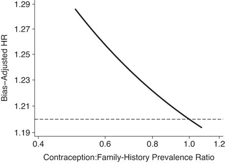
Hazard ratio (HR) bias-adjusted for uncontrolled confounding by family history of breast cancer, assuming the prevalence of family history is 7.74%, the association of family history and incident breast cancer is HR = 2.0, and the association between hormonal contraception and prevalence of family history ranges from 0.5 to 1.08. The horizontal reference line depicts the crude association between hormonal contraception and breast cancer incidence (HR = 1.20).

The results of this QBA are consistent with the results obtained by Mørch et al.: Confounding by family history of postmenopausal breast cancer is unlikely to explain the observed non-null association between the use of hormonal contraception and breast cancer risk. If anything, the association is likely to be slightly larger. This result is consistent with a substantial evidence base (33). However, the methods and assumptions underlying a QBA should be transparent enough to allow replication of results. Further, by focusing on the bias-adjusted effect, rather than the strength of confounding necessary to reduce an observed effect to the null, a more robust scientific conclusion can be drawn.

DISCUSSION

There were common shortcomings in the application of QBA in the preceding examples. First, the authors did not provide bias models relating conventional estimates to bias-adjusted estimates, they did not provide example computations, and they did not provide statistical computing code used for their QBAs. Second, a main limitation was poor selection of values assigned to the parameters of the bias model. In the information bias example, the authors used a specificity of 100% for cases and controls when the internal validation study showed imperfect and differential specificity for controls in the tables used to select the corresponding values of sensitivity. In the selection bias example, the authors assigned a mean of no bias, and then reported that selection bias was unlikely to have affected the study results. In the uncontrolled confounding example, the authors avoided specifying values for most bias parameters, instead examining a wide range of values inconsistent with high-quality evidence. Use of these values showed that uncontrolled confounding was an unlikely threat to validity. Third, there was little text provided in each example to defend the chosen values assigned to the bias parameters. Finally, there was little effort to understand the range of uncertainty associated with the biases; the emphases were on single bias-adjusted estimates of association.

The values to assign to parameters of QBA models are never known with certainty. Choices should be made with the goal of obtaining valid estimates. Choosing exaggerated values that would erase a non-null estimate of association is less productive than choosing defensible values and thereby providing a more valid bias-adjusted estimate. Worse still is choosing values that will suggest that the conventional estimate was not susceptible to bias.

We recognize that the alternative bias analyses we provided could be improved, especially with access to the original data. Our alternatives were meant to follow the methods used by the original authors, while addressing the limitations the original bias analyses shared, as described above. We have not considered the relative utility of different methodological approaches to QBA, which has most recently been debated in the context of the utility of E-values to address uncontrolled confounding (34–40). Most biases can be conceptualized as missing data problems (10), so when original data are available, missing data methods might be the most effective analytical approach.

One utility of QBA is to help explain the role of bias in generating apparently heterogeneous results for a given hypothesis (41), which might otherwise be misinterpreted as poor reproducibility. Suboptimal bias analyses would, however, fail to fulfill this goal. Until QBA becomes more common, community expectations for the presentation, explanation, and interpretation of bias analyses will remain unstable. Attention to good practices, such as those we and others outlined earlier (15), by authors, reviewers, and editors should improve quality, avoid errors, discourage manipulation, and help the application of QBA to reach its optimal utility.

REFERENCES

- 1.Bross I. Misclassification in 2×2 tables. Biometrics. 1954;10(4):478–486. [Google Scholar]
- 2.Bross ID. Spurious effects from an extraneous variable. J Chronic Dis. 1966;19(6):637–647. [DOI] [PubMed] [Google Scholar]
- 3.Cornfield J, Haenszel W, Hammond EC, et al. Smoking and lung cancer: recent evidence and a discussion of some questions. J Natl Cancer Inst. 1959;22(1):173–203. [PubMed] [Google Scholar]
- 4.Greenland S. Basic methods for sensitivity analysis of biases. Int J Epidemiol. 1996;25(6):1107–1116. [PubMed] [Google Scholar]
- 5.Lash TL, Fink AK. Semi-automated sensitivity analysis to assess systematic errors in observational data. Epidemiology. 2003;14(4):451–458. [DOI] [PubMed] [Google Scholar]
- 6.Fox MP, Lash TL, Greenland S. A method to automate probabilistic sensitivity analyses of misclassified binary variables. Int J Epidemiol. 2005;34(6):1370–1376. [DOI] [PubMed] [Google Scholar]
- 7.Greenland S. Multiple-bias modeling for analysis of observational data. J R Stat Soc Ser -Stat Soc. 2005;168(2):267–306. [Google Scholar]
- 8.Lyles RH. A note on estimating crude odds ratios in case-control studies with differentially misclassified exposure. Biometrics. 2002;58(4):1034–1036. [DOI] [PubMed] [Google Scholar]
- 9.Lyles RH, Lin J. Sensitivity analysis for misclassification in logistic regression via likelihood methods and predictive value weighting. Stat Med. 2010;29(22):2297–2309. [DOI] [PMC free article] [PubMed] [Google Scholar]
- 10.Howe CJ, Cain LE, Hogan JW. Are all biases missing data problems? Curr Epidemiol Rep. 2015;2(3):162–171. [DOI] [PMC free article] [PubMed] [Google Scholar]
- 11.MacLehose RF, Gustafson P. Is probabilistic bias analysis approximately Bayesian? Epidemiology. 2012;23(1):151–158. [DOI] [PMC free article] [PubMed] [Google Scholar]
- 12.MacLehose RF, Bodnar LM, Meyer CS, et al. Hierarchical semi-Bayes methods for misclassification in perinatal epidemiology. Epidemiology. 2018;29(2):183–190. [DOI] [PMC free article] [PubMed] [Google Scholar]
- 13.Gustafson P. Measurement Error and Misclassification in Statistics and Epidemiology: Impacts and Bayesian Adjustments. Chapman & Hall/CRC: Boca Raton, Florida; 2003. [Google Scholar]
- 14.Chu R, Gustafson P, Le N. Bayesian adjustment for exposure misclassification in case–control studies. Stat Med. 2010;29(9):994–1003. [DOI] [PubMed] [Google Scholar]
- 15.Jurek AM, Maldonado G, Greenland S, et al. Exposure-measurement error is frequently ignored when interpreting epidemiologic study results. Eur J Epidemiol. 2006;21(12):871–876. [DOI] [PubMed] [Google Scholar]
- 16.Hunnicutt JN, Ulbricht CM, Chrysanthopoulou SA, et al. Probabilistic bias analysis in pharmacoepidemiology and comparative effectiveness research: a systematic review. Pharmacoepidemiol Drug Saf. 2016;25(12):1343–1353. [DOI] [PMC free article] [PubMed] [Google Scholar]
- 17.Greenland S, Lash TL. Bias analysis. In: Rothman KJ, Greenland S, Lash TL, eds. Modern Epidemiology. 3rd ed. Philadelphia: Lippincott Williams & Wilkins; 2008:345–380. [Google Scholar]
- 18.Greenland S. Invited commentary: the need for cognitive science in methodology. Am J Epidemiol. 2017;186(6):639–645. [DOI] [PubMed] [Google Scholar]
- 19.Lash TL, Fox MP, MacLehose RF, et al. Good practices for quantitative bias analysis. Int J Epidemiol. 2014;43(6):1969–1985. [DOI] [PubMed] [Google Scholar]
- 20.Chien C, Li CI, Heckbert SR, et al. Antidepressant use and breast cancer risk. Breast Cancer Res Treat. 2006;95(2):131–140. [DOI] [PubMed] [Google Scholar]
- 21.Boudreau DM, Daling JR, Malone KE, et al. A validation study of patient interview data and pharmacy records for antihypertensive, statin, and antidepressant medication use among older women. Am J Epidemiol. 2004;159(3):308–317. [DOI] [PubMed] [Google Scholar]
- 22.Armstrong BK, White E, Saracci R. Principles of Exposure Measurement in Epidemiology. New York, New York: Oxford University Press; 1992: (Principles of exposure measurement in epidemiology. Monographs in epidemiology and biostatistics; vol. 21). [Google Scholar]
- 23.Greenland S. Variance estimation for epidemiologic effect estimates under misclassification. Stat Med. 1988;7(7):745–757. [DOI] [PubMed] [Google Scholar]
- 24.di Forti M, Quattrone D, Freeman TP, et al. The contribution of cannabis use to variation in the incidence of psychotic disorder across Europe (EU-GEI): a multicentre case-control study. Lancet Psychiatry. 2019;6(5):427–436. [DOI] [PMC free article] [PubMed] [Google Scholar]
- 25.di Forti M, Morgan C, Selten J-P, et al. High-potency cannabis and incident psychosis: correcting the causal assumption—authors’ reply. Lancet Psychiatry. 2019;6(6):466–467. [DOI] [PubMed] [Google Scholar]
- 26.Greenland S, Mickey R. Closed form and dually consistent methods for inference on strict collapsibility in 2x2xK and 2xJxK tables. Appl Stat. 1988;37(3):335–343. [Google Scholar]
- 27.Mørch LS, Skovlund CW, Hannaford PC, et al. Contemporary hormonal contraception and the risk of breast cancer. N Engl J Med. 2017;377(23):2228–2239. [DOI] [PubMed] [Google Scholar]
- 28.Schlesselman JJ. Assessing effects of confounding variables. Am J Epidemiol. 1978;108(1):3–8. [PubMed] [Google Scholar]
- 29.Lin DY, Psaty BM, Kronmal RA. Assessing the sensitivity of regression results to unmeasured confounders in observational studies. Biometrics. 1998;54(3):948–963. [PubMed] [Google Scholar]
- 30.Mørch LS, Hannaford PC, Lidegaard Ø. Contemporary hormonal contraception and the risk of breast cancer. N Engl J Med. 2018;378(13):1265–1266. [DOI] [PubMed] [Google Scholar]
- 31.Pharoah PD, Day NE, Duffy S, et al. Family history and the risk of breast cancer: a systematic review and meta-analysis. Int J Cancer. 1997;71(5):800–809. [DOI] [PubMed] [Google Scholar]
- 32.Ramsey SD, Yoon P, Moonesinghe R, et al. Population-based study of the prevalence of family history of cancer: implications for cancer screening and prevention. Genet Med. 2006;8(9):571–575. [DOI] [PMC free article] [PubMed] [Google Scholar]
- 33.Hunter DJ. Oral contraceptives and the small increased risk of breast cancer. N Engl J Med. 2017;377(23):2276–2277. [DOI] [PubMed] [Google Scholar]
- 34.Ioannidis JP, Tan YJ, Blum MR. Limitations and misinterpretations of E-values for sensitivity analyses of observational studies. Ann Intern Med. 2019;170(2):108–111. [DOI] [PubMed] [Google Scholar]
- 35.Blum MR, Tan YJ, Ioannidis JPA. Use of E-values for addressing confounding in observational studies—an empirical assessment of the literature. Int J Epidemiol. 2020;49(5):1482–1494. [DOI] [PubMed] [Google Scholar]
- 36.Kaufman JS. Commentary: cynical epidemiology. Int J Epidemiol. 2020;49(5):1507–1508. [DOI] [PubMed] [Google Scholar]
- 37.Poole C. Commentary: continuing the E-value's post-publication peer review. Int J Epidemiol. 2020;49(5):1497–1500. [DOI] [PMC free article] [PubMed] [Google Scholar]
- 38.Greenland S. Commentary: an argument against E-values for assessing the plausibility that an association could be explained away by residual confounding. Int J Epidemiol. 2020;49(5):1501–1503. [DOI] [PubMed] [Google Scholar]
- 39.VanderWeele TJ, Mathur MB, Ding P. Correcting misinterpretations of the E-value. Ann Intern Med. 2019;170(2):131–132. [DOI] [PubMed] [Google Scholar]
- 40.VanderWeele TJ, Mathur MB. Commentary: developing best-practice guidelines for the reporting of E-values. Int J Epidemiol. 2020;49(5):1495–1497. [DOI] [PMC free article] [PubMed] [Google Scholar]
- 41.Lash TL. The harm done to reproducibility by the culture of null hypothesis significance testing. Am J Epidemiol. 2017;186(6):627–635. [DOI] [PubMed] [Google Scholar]