Reflection on modern methods: causal inference considerations for heterogeneous disease etiology

Abstract

Molecular pathological epidemiology research provides information about pathogenic mechanisms. A common study goal is to evaluate whether the effects of risk factors on disease incidence vary between different disease subtypes. A popular approach to carrying out this type of research is to implement a multinomial regression in which each of the non-zero values corresponds to a bona fide disease subtype. Then, heterogeneity in the exposure effects across subtypes is examined by comparing the coefficients of the exposure between the different subtypes. In this paper, we explain why this common method potentially cannot recover causal effects, even when all confounders are measured, due to a particular type of selection bias. This bias can be explained by recognizing that the multinomial regression is equivalent to a series of logistic regressions; each compares cases of a certain subtype to the controls. We further explain how this bias arises using directed acyclic graphs and we demonstrate the potential magnitude of the bias by analysis of a hypothetical data set and by a simulation study.

Key Messages

• The multinomial regression approach has been the main statistical tool for studying etiologic heterogeneity with categorical outcomes representing disease subtypes.

• Causal interpretation of the results of the multinomial regression approach has been missing from the discussion.

• Selection bias is likely to arise in etiologic heterogeneity studies due to unmeasured variables associated with all disease subtypes.

• Using potential outcomes, directed acyclic graphs, a hypothetical data set and simulations, we demonstrate how this bias arises and study its magnitude.

Introduction

Modern disease etiology research seeks to identify and characterize the pathogenic effects of risk factors that may vary according to pathways (processes) to specific disease subtypes.^1–8 Molecular pathological epidemiology (MPE) has been developed as an interdisciplinary science that integrates molecular pathological methods into epidemiologic and statistical methods to gain more mechanistic insights into disease etiologies.^1–8

Using the MPE approach, evidence for the differential effects of exposures on various tumour subtypes has been shown. For example, high-level microsatellite instability (MSI) is one well-established feature observed in ∼15% of colorectal cancer (CRC) cases.⁹ Existing results indicate that the association between cigarette smoking and CRC is stronger for the MSI-high subtype than for the non-MSI-high subtype.^10,11

Heterogeneity in risk factor effects on categorical disease outcomes is usually studied using a multinomial regression approach.^4,12,13 Recently, there has been some debate on whether the multinomial regression model is suitable for studying heterogeneity.^14,15 While important, a key issue is missing from this discussion. Here, we focus on whether the results of the standard analysis can yield causal interpretation and demonstrate that a specific form of selection bias is likely to arise when conducting MPE-type research.

The multinomial regression approach for disease heterogeneity

Let $i$ index individuals, $Y_i=0$ denote a disease-free participant, $Y_i=1$ a non-MSI-high subtype CRC case and $Y_i=2$ an MSI-high subtype CRC case. Let $A_i=1$ denote an ‘ever-smoker’ and $A_i=0$ a ‘never-smoker’. Adjustment for confounders ${\mathit{X}}_i$ is typically carried out^4,16 by fitting the multinomial regression model

$$\mathit{log}\left[\frac{Pr\left(Y_i=k|A_i,{\mathit{X}}_i\right)}{Pr\left(Y_i=0|A_i,{\mathit{X}}_i\right)}\right]={\stackrel{\sim }{\alpha }}_k+{\stackrel{\sim }{\beta }}_k{A}_i+{\stackrel{\sim }{\gamma }\mathrm{\text{'}}}_k{\mathit{X}}_i$$ (1)

for $k=\mathrm{1,2}$ and $Pr\left(Y_i=0|A_i,{\mathit{X}}_i\right)=1-Pr\left(Y_i=1|A_i,{\mathit{X}}_i\right)-Pr\left(Y_i=2|A_i,{\mathit{X}}_i\right)$.

The association parameter $\text{exp}\left({\stackrel{\sim }{\mathrm{\beta }}}_{\mathrm{k}}\right)$ represents the odds ratio (OR) between the exposure and the subtype $k$ outcome vs being disease-free $\frac{Pr\left(Y_i=k|A_i=1,{\mathit{X}}_{\mathbf{i}}\right)}{Pr\left(Y_i=0|A_i=1,{\mathit{X}}_i\right)}\frac{Pr\left(Y_i=0|A_i=0,{\mathit{X}}_i\right)}{Pr\left(Y_i=k|A_i=0,{\mathit{X}}_i\right)}.$⁴ We will refer to this parameter as the relative risk (RR) when appropriate, as in rare-disease scenarios. This parameter is sometimes implicitly interpreted as the causal effect of the exposure on the subtype $k$ outcome. Heterogeneity is studied by comparing $\text{exp}\hspace{0.17em}$(${\stackrel{\sim }{\beta }}_1)$ to $\text{exp}\left({\stackrel{\sim }{\beta }}_2\right)$. An observed discrepancy provides information on whether a certain exposure has a differential effect on the development of cancer subtypes.

The multinomial regression Model (1) is equivalent to two separate logistic-regression models; each compares a different disease subtype to the healthy participants. That is, the parameters ${\stackrel{\sim }{\alpha }}_k,{\stackrel{\sim }{\beta }}_k\mathrm{ }\mathrm{and}\mathrm{ }{\stackrel{\sim }{\gamma }}_k$ are identical to the parameters of a logistic regression model for subtype-specific cases when participants with other disease subtypes are excluded.

Formulation in causal language

To examine the causal interpretation of parameters estimated from the models above, we first formulate the relevant potential outcomes.¹⁷ Let $Y^{\left(1\right)}\left(0\right)$ indicate a non-MSI-high CRC under the value $A=0$ (never smoked) and let $Y^{\left(1\right)}\left(1\right)$ be the indicator of having a non-MSI-high case under the value $A=1$ (ever smoked). Similarly, let $Y^{\left(2\right)}\left(a\right)$ be the indicator of having an MSI-high CRC under $A=a$. To clarify, for controls $Y^{\left(1\right)}\left(a\right)=Y^{\left(2\right)}\left(a\right)=0$. Furthermore, each diseased individual may experience one specific subtype only, i.e. $Y^{\left(1\right)}\left(a\right)=1$ implies $Y^{\left(2\right)}\left(a\right)=0$ and, vice versa, $Y^{\left(2\right)}\left(a\right)=1$ implies $Y^{\left(1\right)}\left(a\right)=0.$

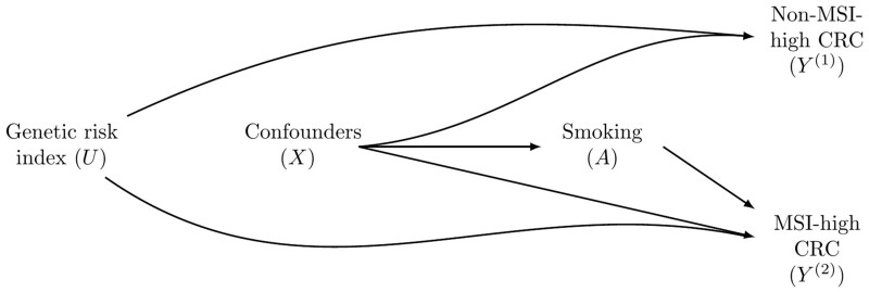
Because the subtypes are mutually exclusive, the foregoing analysis of etiological heterogeneity across the subtypes is inherently a competing-risks setup.^18–22 As in many studies involving competing risks, two important issues arise. First, the study focuses on the effects of an exposure on both competing events (i.e. both subtypes) and the difference between these two effects. Second, since the study focuses on the same disease, partitioned into subtypes, there may be unmeasured person-specific covariates $U$ that are strongly associated with the risk for both subtypes (e.g. genetic factors). The causal directed acyclic graph (Figure 1) illustrates this scenario, with smoking having no effect on a non-MSI-high CRC, but it does increase the risk for an MSI-high CRC.

Figure 1.

A directed acyclic graph presenting the potential selection bias when studying exposure effects according to microsatellite instability (MSI) status. In this directed acyclic graph, smoking (A, ever vs never) only affects MSI-high CRC. Nevertheless, a non-zero effect estimate is expected for smoking effect on non-MSI-high CRC because the analysis is conditioned on being free of MSI-high CRC ($Y^{\left(2\right)}=0$), opening a non-causal path going through the genetic-risk index ($U$).

With potential outcomes clearly defined, we can investigate what causal effects, if any, can be estimated. The first notion is that a contrast of the subtype-specific risks $Pr\left[Y^{\left(k\right)}\left(1\right)=1\right]$ with $Pr\left[Y^{\left(k\right)}\left(0\right)=1\right]$, known as the total effect,²¹ may not provide the desirable scientific knowledge. It might be that $Pr\left[Y^{\left(1\right)}\left(1\right)=1\right]\ne Pr\left[Y^{\left(1\right)}\left(0\right)=1\right]$ simply because $A$ affects subtype $2$.$\mathrm{ }$Therefore, it has been recommended to consider the total effect of all events to identify such potential cases. In MPE studies, researchers have been using multinomial regression Model (1), essentially comparing one subtype of patients with controls while excluding cases with different subtypes.⁴ However, $\text{exp}\left({\stackrel{\sim }{\beta }}_k\right)$ can be very misleading. Consider the following multinomial regression model, which is consistent with Figure 1:

$$\mathit{log}\left[\frac{Pr\left(Y_i=k|A_i,{\mathit{X}}_i,\mathrm{ }{U}_i\right)}{Pr\left(Y_i=0|A_i,{\mathit{X}}_{\mathit{i}},\mathrm{ }{U}_i\right)}\right]={\alpha }_k+{\beta }_k{A}_i+{\mathit{\gamma }\mathrm{\text{'}}}_k{\mathit{X}}_i+{\theta }_k{U}_i,$$ (2)

for $k=\mathrm{1,2}$, and $Pr\left(Y_i=0|A_i,{\mathit{X}}_i,U_i\right)=1-Pr\left(Y_i=1|A_i,{\mathit{X}}_i,U_i\right)-Pr\left(Y_i=2|A_i,{\mathit{X}}_i,U_i\right)$. In Figure 1, the absence of an arrow from $A$ to $Y^{\left(1\right)}$ implies that ${\beta }_1=0$. If e.g. $U$ is a genetic risk index increasing the risks of both subtypes, then ${\theta }_1>0$ and ${\theta }_2>0$.

There are three potential reasons why $\text{exp}\left({\stackrel{\sim }{\beta }}_k\right)$, the OR in Model (1), which ignores $U$, the common risk factor for both subtypes, is not generally equal to $\text{exp}\left({\beta }_k\right)$, the OR in Model (2), where $U$ is adjusted for. The first reason is the non-collapsibility of the OR.²³ The second reason is that, if the true model is the full model [Equation (2)], then the reduced model [Equation (1)] is mis-specified, as the logit link function is not expected to hold for the reduced model, especially if the effect of $A$ is strong.²⁴ The third reason is the selection bias depicted in Figure 1 and explained below.

Since each cancer subtype is a rare disease, the first two problems are relatively negligible. However, even for rare diseases, $\text{exp}\left({\stackrel{\sim }{\beta }}_1\right)$, the OR representing the exposure–subtype 1 relationship in Model (1), is not expected to be equal to $\text{exp}\left({\beta }_1\right)$ in Model (2). In each of these logistic regression models, only the subset of the participants free of the other disease subtypes is included. For example, when studying the effect of smoking $\left(A\right)$ on non-MSI- high CRC ($Y^{\left(1\right)}$), the analysis is conditioned on $Y^{\left(2\right)}=0$ (MSI-high CRC cases are excluded), which opens a back-door path¹⁷ between $A$ and $Y^{\left(1\right)}$. Consider the scenario $\text{exp}\hspace{0.17em}\left({\beta }_1\right)=1,\mathrm{ }\hspace{0.17em}\text{exp}\hspace{0.17em}\left({\beta }_2\right)>1,{\theta }_k>0$. Because $\text{exp}\left({\stackrel{\sim }{\beta }}_1\right)$ is the same as the exponentiated logistic regression coefficient of A in a logistic regression comparing non-MSI-high CRC patients with controls, it is calculated in the subpopulation created by ignoring MSI-high CRC patients. However, in this subpopulation, the ever-smokers ($A=1)$ have, on average, a lower $U$ than the never-smokers $(A=0)$. Therefore, when fitting Model (1), it would appear as if smoking has a protective effect against a non-MSI-high CRC, whereas the reality is that smoking has no effect on this subtype [$\text{exp}\hspace{0.17em}\left({\beta }_1\right)=1$]. This source of bias is expected in etiologic heterogeneity studies because unmeasured common causes of both disease subtypes are likely to exist.

Under the example described above, selection bias is expected for the effect on non-MSI-high CRC but not for the effect on MSI-high CRC. Conditioning on $Y^{\left(1\right)}=0$ does not open a non-causal path between A and $Y^{\left(2\right)}$ (Figure 1).

Unmeasured factors associated with both subtypes but not with the exposure are ubiquitous. When studying age at menarche in relation to breast cancer (BC), single nucleotide polymorphisms (SNPs) have been found to have a consistent association with all BC subtypes (e.g. SNP rs4415084) or stronger, heterogenous associations with nearly all subtypes (e.g. SNPs rs3104746 and rs2981578).²⁵ However, to our knowledge, none of these SNPs has been found to explain age at menarche.^26,27 Another example involves non-genetic factors. Aspirin-taking has been associated with reduced risks for MSI-high and non-MSI-high CRC subtypes.²⁸ However, not all exposures are associated with aspirin-taking, which is not always available.

Selection bias may also arise when $U$ is a post-exposure mediator between the exposure and both disease subtypes (Figure 2). For example, when researchers study the effect of age at menarche on BC, subtyped by estrogen receptor status, mammographic density is a potential mediator.²⁴ In this case, $\text{exp}\hspace{0.17em}\left({\beta }_k\right)$ in Model (2) is no longer the causal effect of the exposure on subtype $k$. This problem persists even if $U$ is observed, as adjustment for mammographic density to avoid the selection bias will block the effect of age at menarche mediated by mammographic density. Therefore, alternative approaches are desirable, including targeting the total effect, defining a survivor average causal effect^29,30 or leveraging the separable effects paradigm²² (see the ‘Discussion’ section).

Figure 2.

A directed acyclic graph presenting a second potential selection bias mechanism when studying exposure effects according to different subtypes. In this directed acyclic graph, the age at menarche (A) affects both estrogen receptor positive (ESR1-POS) and estrogen receptor negative (ESR1-NEG) breast cancer (BC) through the mediator mammographic density (U). Age at menarche also directly affects ESR1-NEG BC. A biased estimate is expected for the age-at-menarche total effect on ESR1-POS BC because the analysis is conditioned on being free of ESR1-NEG BC ($Y^{\left(2\right)}=0$), opening the non-causal path $A\to Y^{\left(2\right)}\leftarrow U\to Y^{\left(1\right)}$. Adjustment for $U$ to block the non-causal path would also block the effect that age at menarche has on ESR1-POS BC, leading to ${\beta }_1$ from Model (2) not corresponding to the causal effect of age at menarche on ESR1-POS BC.

A hypothetical data set

We present a hypothetical example that can be also analysed by the reader to illustrate the selection bias. Table 1 presents data for a hypothetical population. In addition to smoking status $\left(A\right)$, there is also a continuous unmeasured $U$ that is associated with the outcome but not with $A$. For illustrative purposes, there is no confounding in this example. A logistic regression of $Y=1$ vs $Y=0$ on $U$ and $A$ yields an estimated RR $\text{exp}\left({\widehat{\beta }}_1\right)=1.0$ [95% confidence interval (CI): 0.93, 1.08]. This corresponds to ${\hspace{0.17em}\text{exp}(\beta }_1)$ in Model (2). However, as $U$ is unobserved by researchers, the logistic regression of $Y=1$ vs $Y=0$ would only include $A$, leading to a biased effect estimate $\text{exp}\left({\beta \sim ^}_1\right)=0.88 < 1$ (95% CI: 0.82, 0.95).

Table 1.

Data on a hypothetical population of size 100 000 including a risk score index (U, continuous with values rounded), smoking status (A, 1: ever-smoker, 0: never-smoker) and disease status with subtypes defined by microsatellite (MSI) (Y, 0: Healthy, 1: Non-MSI-high CRC, 2: MSI-high CRC). Positive and negative values of U are associated with increased and decreased risk, respectively.

Genetic-risk index$\mathrm{ }\left(U\right)$	Smoking status $\left(A\right)$	Outcome $\left(Y\right)$	Count
−2	0	0	10 000
−2	0	1	10
−2	0	2	10
−2	1	0	10 000
−2	1	1	10
−2	1	2	20
−1	0	0	9800
−1	0	1	10
−1	0	2	10
−1	1	0	10 000
−1	1	1	10
−1	1	2	50
0	0	0	9700
0	0	1	60
0	0	2	60
0	1	0	9500
0	1	1	100
0	1	2	200
1	0	0	9500
1	0	1	400
1	0	2	350
1	1	0	9000
1	1	1	300
1	1	2	900
2	0	0	7500
2	0	1	1200
2	0	2	1300
2	1	0	6000
2	1	1	1000
2	1	2	3000

Illustration of the problem by simulations

We further illustrate and quantify the magnitude of the bias using simulations. In all scenarios considered, 1000 data sets were simulated. For simplicity, data were simulated from a version of Model (2) with no confounders and with a single normally distributed unmeasured risk factor $U\sim N\left(\mathrm{0,1}\right)$. Initially, the exposure did not affect the first subtype [$\text{exp}\hspace{0.17em}\left({\beta }_1\right)=1]$ and we varied the values of $\text{exp}\left({\beta }_2\right)$ and of $\text{exp}\left({\theta }_1\right)=\text{exp}\left({\theta }_2\right)=\text{exp}(\theta )$. The exposure, $A$, was randomized with $\mathrm{Pr}(A = 1)=0.5$. To mimic real-life rare-disease data, the sample size was taken to be $n=50\mathrm{ }000$, with incidence proportions of 0.3%–1% (subtype 1) and 0.9%–4.3% (subtype 2).

For each simulated data set, we fit Model (1). For subtype 1, the mean estimated RR was nearly always <1 and the absolute bias increased as the value of $\text{exp}(\theta )$ increased (Figure 3). For subtype 2, the mean estimated RR was lower than the true unconditional RR (Figure 4), but this was due to the lack of collapsibility of the logistic function.^23,24 Additional simulations confirmed this claim (Section 1 of the Supplementary Material, available as Supplementary data at IJE online).

Figure 3.

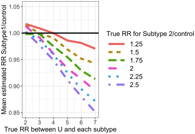
Mean estimated subtype 1-specific relative risk (RR) in simulations when using Model (1) while data are simulated under Model (2). True (conditional) RR between U and each subtype is simply $\exp (\theta )$ in Model (2) and represents the strength of the association between $U$ and $Y^{\left(1\right)}$ and between $U$ and $Y^{\left(2\right)}.$

Figure 4.

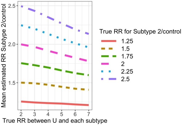
Mean estimated subtype 2-specific relative risk (RR) in simulations when using Model (1) while data are simulated under Model (2). True (conditional) RR between U and subtype is simply $exp(\theta )$ in Model (2) and represents the strength of the association between $U$ and $Y^{\left(1\right)}$ and between $U$ and $Y^{\left(2\right)}.$

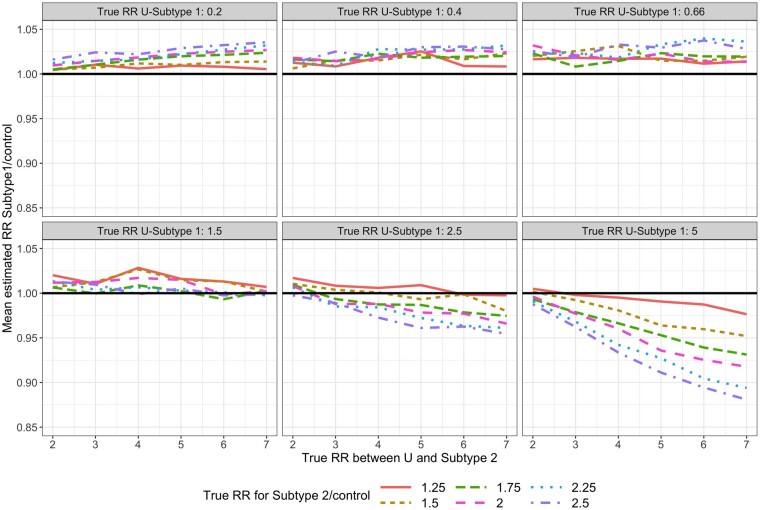
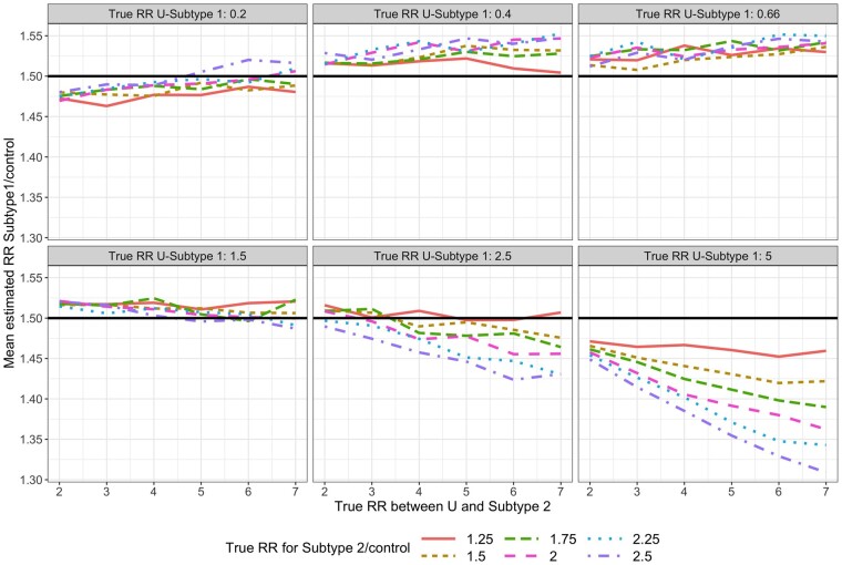
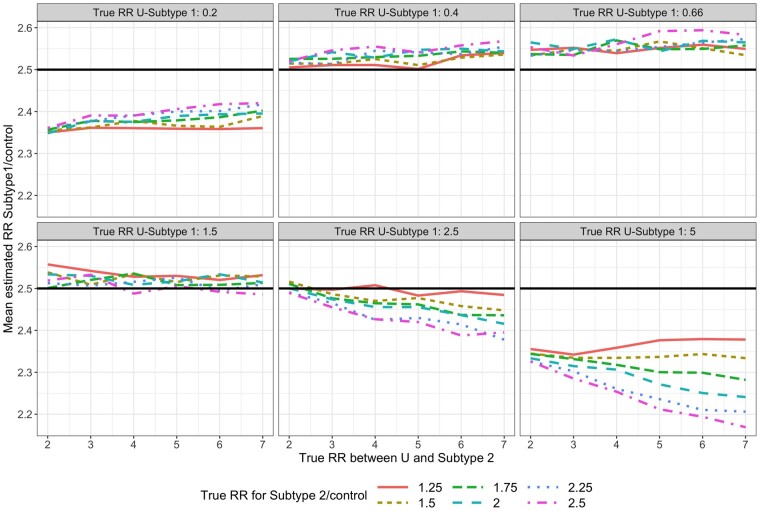
The magnitude and direction of the bias depend on the relationships between U, A and each of the disease subtypes. Therefore, we conducted further simulations, varying the values of ${\beta }_1,{\beta }_2,{\theta }_1\mathrm{ }\mathrm{and}\mathrm{ }{\theta }_2$. The subtype 1 RR bias can be positive or negative (Figures 5–7 and Supplementary Figures 4–6, available as Supplementary data at IJE online). In most scenarios, the absolute bias increased as the $A-Y^{\left(2\right)}$ and $U-Y^{\left(2\right)}$ relationships were stronger. When both non-collapsibility and selection bias were present, the patterns were more complex (Figures 6 and 7). Section 2 of the Supplementary Material, available as Supplementary data at IJE online, presents more details.

Figure 5.

Mean estimated subtype 1-specific relative risk (RR) in simulations when using Model (1) while data are simulated under Model (2). True RR is 1. True (conditional) RR between U and each subtype is simply $exp\left({\theta }_k\right)$ in Model (2).

Figure 6.

Mean estimated subtype 2-specific relative risk (RR) in simulations when using Model (1) while data are simulated under Model (2). True RR is 1.5. True (conditional) RR between U and each subtype is simply $exp\left({\theta }_k\right)$ in Model (2).

Figure 7.

Mean estimated subtype 2-specific relative risk (RR) in simulations when using Model (1) while data are simulated under Model (2). True RR is 2.5. True (conditional) RR between U and each subtype is simply $exp\left({\theta }_k\right)$ in Model (2).

We extended the simulation studies for non-rare-disease scenarios. The results (Section 3 of the Supplementary Material, available as Supplementary data at IJE online) were qualitatively similar, with larger discrepancies between the estimated $\text{exp}\left({\stackrel{\sim }{\beta }}_2\right)$ and $\text{exp}\left({\beta }_2\right)$, presumably due to the non-collapsibility of the logistic regression.

Finally, in Section 4 of the Supplementary Material, available as Supplementary data at IJE online, we report the results of an additional simulation study for the scenarios in which $U$ is a mediator between $A$ and both subtypes. This simulation verified that the multinomial regression approach does not uncover the total effect of $A$ on a specific subtype.

Discussion

In this paper, we formalized and reviewed the question of causal inference for etiologic heterogeneity studies. We demonstrated that selection bias is expected to arise in these studies when the multinomial regression approach is used. R code to recreate our results is available online (https://github.com/daniel258/CausalMPE). In some specialized cases, selection bias is not expected. When studying the effect on subtype $1$, no selection bias is expected if the following multiplicative model holds: $Pr\left(Y^{\left(2\right)}=0|A=a,U=u\right)=f\left(a\right)g\left(u\right)$, for some functions $f,g$, i.e. if $U$ does not modify the effect $A$ has on being free of subtype 2.³¹

Competing risks,^18–22 as in the case of multiple disease subtypes, present a challenge of choosing which causal effect to study. Recently, the different potential strategies, including risk-based and hazard-based comparisons, and their analogue causal effects (when those exist) were thoroughly investigated and reviewed.²¹

At face value, an alternative approach is the method developed by Sun et al.,¹⁴ who used a logistic model for $\frac{\mathrm{Pr}(Y_i=k|A_i,\mathrm{ }{\mathit{X}}_i)}{\mathrm{Pr}(Y_i\ne k|A_i,\mathrm{ }{\mathit{X}}_{\mathrm{i}})}$ rather than for $\frac{\mathrm{Pr}({\mathrm{Y}}_{\mathrm{i}}=k|A_i,{\mathit{X}}_i)}{\mathrm{Pr}(Y_i=0|A_i,{\mathit{X}}_i)}$ and utilized a Bayesian approach to ensure that the probabilities sum to one. Crucially, this approach does not suffer the selection bias described in this paper. Furthermore, it corresponds to a well-defined causal contrast of $\mathrm{Pr}\left[Y^{\left(k\right)}\left(1\right)=1\right]$ and $\mathrm{Pr}[Y^{\left(k\right)}\left(0\right)=1]$ known as the total effect. However, the exposure effect on subtype $k$ represented by this contrast could be the result of the exposure effect on other subtypes.²¹ For example, the total effect might be non-null if there are study participants who would have been diagnosed with subtype $k$ when unexposed and other subtypes when exposed. In this case, the total effect does not reveal the reason for the seemingly protective effect against subtype $k$.

Other potential strategies include the survival average causal effect,^29,30 which is the causal effect of the exposure on one subtype, within the population who would be free of the other subtype under both exposure levels. Alternatively, the recently proposed separable effects paradigm²² could be promising, although it would require a deeper knowledge about the causal mechanisms leading to each tumour-subtype formulation.

In conclusion, we have shed light on an understudied and important issue in the study of pathogenic heterogeneity. We expect an immediate impact on the way in which results are interpreted. We end this paper with a call for alternative methods targeting well-defined causal effects in MPE-type analyses.

Supplementary data

Supplementary data are available at IJE online.

References

- 1.Jung S, Wang M, Anderson K. et al. Alcohol consumption and breast cancer risk by estrogen receptor status: In a pooled analysis of 20 studies. Int J Epidemiol 2016;45:916–28. [DOI] [PMC free article] [PubMed] [Google Scholar]
- 2.Ogino S, Giovannucci E.. Commentary: Lifestyle factors and colorectal cancer microsatellite instability-molecular pathological epidemiology science, based on unique tumour principle. Int J Epidemiol 2012;41:1072–74. [DOI] [PMC free article] [PubMed] [Google Scholar]
- 3.Ogino S, Nishihara R, VanderWeele TJ. et al. The role of molecular pathological epidemiology in the study of neoplastic and non-neoplastic diseases in the era of precision medicine. Epidemiology 2016;27:602–11. [DOI] [PMC free article] [PubMed] [Google Scholar]
- 4.Wang M, Spiegelman D, Kuchiba A. et al. Statistical methods for studying disease subtype heterogeneity. Stat Med 2016;35:782–800. [DOI] [PMC free article] [PubMed] [Google Scholar]
- 5.Murphy N, Jenab M, Gunter MJ.. Adiposity and gastrointestinal cancers: epidemiology, mechanisms and future directions. Nat Rev Gastroenterol Hepatol 2018;15:659–70. [DOI] [PubMed] [Google Scholar]
- 6.Gunter MJ, Alhomoud S, Arnold M. et al. Meeting report from the joint IARC-NCI international cancer seminar series: a focus on colorectal cancer. Ann Oncol 2019;30:510–19. [DOI] [PMC free article] [PubMed] [Google Scholar]
- 7.Zakhari S, Hoek JB.. Epidemiology of moderate alcohol consumption and breast cancer: Association or causation? Cancers (Basel). 2018;10:349. [DOI] [PMC free article] [PubMed] [Google Scholar]
- 8.Ogino S, Nowak JA, Hamada T, Milner DA, Nishihara R.. Insights into pathogenic interactions among environment, host, and tumor at the crossroads of molecular pathology and epidemiology. Annu Rev Pathol Mech Dis 2019;14:83–103. [DOI] [PMC free article] [PubMed] [Google Scholar]
- 9.Inamura K.Colorectal cancers: An update on their molecular pathology. Cancers (Basel) 2018;10:26. [DOI] [PMC free article] [PubMed] [Google Scholar]
- 10.Carr PR, Alwers E, Bienert S. et al. Lifestyle factors and risk of sporadic colorectal cancer by microsatellite instability status: a systematic review and meta-analyses. Ann Oncol 2018;29:825–34. [DOI] [PubMed] [Google Scholar]
- 11.Amitay EL, Carr PR, Jansen L. et al. Smoking, alcohol consumption and colorectal cancer risk by molecular pathological subtypes and pathways. Br J Cancer 2020;122:1604–10. [DOI] [PMC free article] [PubMed] [Google Scholar]
- 12.Nevo D, Zucker DM, Tamimi RM, Wang M.. Accounting for measurement error in biomarker data and misclassification of subtypes in the analysis of tumor data. Stat Med 2016;35:5686–700. [DOI] [PMC free article] [PubMed] [Google Scholar]
- 13.Zabor EC, Begg CB.. A comparison of statistical methods for the study of etiologic heterogeneity. Stat Med 2017;36:4050–60. [DOI] [PMC free article] [PubMed] [Google Scholar]
- 14.Sun B, VanderWeele T, Tchetgen Tchetgen EJ.. A multinomial regression approach to model outcome heterogeneity. Am J Epidemiol 2017;186:1097–103. [DOI] [PMC free article] [PubMed] [Google Scholar]
- 15.Begg CB, Seshan VE, Zabor EC.. Re: A multinomial regression approach to model outcome heterogeneity. Am J Epidemiol 2018;187:1129–30. [DOI] [PMC free article] [PubMed] [Google Scholar]
- 16.Chatterjee N.A two-stage regression model for epidemiological studies with multivariate disease classification data. J Am Stat Assoc 2004;99:127–38. [Google Scholar]
- 17.Hernán MA, Robins JM.. Causal Inference: What If. Boca Raton: Chapman & Hall/CRC, 2020. [Google Scholar]
- 18.Putter H, Fiocco M, Geskus RB.. Tutorial in biostatistics: competing risk and multi-state models. Statist Med 2007;26:2389–430. [DOI] [PubMed] [Google Scholar]
- 19.Geskus RB.Data Analysis with Competing Risks and Intermediate States. Data Analysis with Competing Risks and Intermediate States. New York: Chapman and Hall/CRC, 2015. [Google Scholar]
- 20.Nevo D, Nishihara R, Ogino S, Wang M.. The competing risks Cox model with auxiliary case covariates under weaker missing-at-random cause of failure. Lifetime Data Anal 2018;24:425–42. [DOI] [PMC free article] [PubMed] [Google Scholar]
- 21.Young JG, Stensrud MJ, Tchetgen Tchetgen EJ, Hernán MA.. A causal framework for classical statistical estimands in failure-time settings with competing events. Stat Med 2020;39:1199–236. [DOI] [PMC free article] [PubMed] [Google Scholar]
- 22.Stensrud MJ, Young JG, Didelez V, Robins JM, Hernán MA.. Separable effects for causal inference in the presence of competing events. J Am Stat Assoc 2020;(just-accepted):1–23. [Google Scholar]
- 23.Greenland S, Robins JM et al.. Confounding and collapsibility in causal inference. Stat Sci 1999;14:29–46. [Google Scholar]
- 24.Nevo D, Liao X, Spiegelman D.. Estimation and inference for the mediation proportion. Int J Biostat 2017;13. 10.1515/ijb-2017-0006 [DOI] [PMC free article] [PubMed] [Google Scholar]
- 25.O'Brien KM, Cole SR, Engel LS. et al. Breast cancer subtypes and previously established genetic risk factors: a Bayesian approach. Cancer Epidemiol Biomarkers Prev 2014;23:84–97. [DOI] [PMC free article] [PubMed] [Google Scholar]
- 26.Elks CE, Perry JRB, Sulem P; The GIANT Consortium et al. Thirty new loci for age at menarche identified by a meta-analysis of genome-wide association studies. Nat Genet 2010;42:1077–85. [DOI] [PMC free article] [PubMed] [Google Scholar]
- 27.Perry JRB, Day F, Elks CE; Australian Ovarian Cancer Study et al. Parent-of-origin-specific allelic associations among 106 genomic loci for age at menarche. Nature 2014. Oct 2;514:92–97. [DOI] [PMC free article] [PubMed] [Google Scholar]
- 28.Amitay EL, Carr PR, Jansen L. et al. Association of aspirin and nonsteroidal anti-inflammatory drugs with colorectal cancer risk by molecular subtypes. J Natl Cancer Inst 2019. May 1;111:475–83. [DOI] [PubMed] [Google Scholar]
- 29.Frangakis CE, Rubin DB.. Principal stratification in causal inference. Biometrics 2002;58:21–29. [DOI] [PMC free article] [PubMed] [Google Scholar]
- 30.Chiba Y, VanderWeele TJ.. A simple method for principal strata effects when the outcome has been truncated due to death. Am J Epidemiol 2011;173:745–51. [DOI] [PMC free article] [PubMed] [Google Scholar]
- 31.Hernán MA, Hernández-Díaz S, Robins JM.. A structural approach to selection bias. Epidemiology 2004;15:615–25. [DOI] [PubMed] [Google Scholar]
Associated Data
This section collects any data citations, data availability statements, or supplementary materials included in this article.