

Abstract
Purpose:
Slice-selective, gradient-crushed, transient-state sequences such as those used in magnetic resonance fingerprinting (MRF) relaxometry are sensitive to slice profile effects. While balanced steady-state free precession MRF profile effects have been studied, less attention has been given to gradient-crushed MRF forms. Extensions of the extended phase graph (EPG) formalism are proposed, called slice-selective EPG (ssEPG), that model slice profile effects.
Theory and Methods:
The hard-pulse approximation to slice-selective excitation in the spatial domain is reformulated in k-space. Excitation is modeled by standard EPG shift and transition operators. This ssEPG modeling is validated against Bloch simulations and phantom slice profile measurements. ssEPG relaxometry accuracy and variability are compared with other EPG methods in phantoms and human leg in vivo. The role of ΔB0 interactions with slice profile and gradient crushers are investigated.
Results:
Simulations and slice profile measurements show that ssEPG can model highly dynamic slice profile effects of gradient-crushed sequences. The MRF ssEPG T2 estimates over 0 < T2 < 100 ms improve accuracy by > 10 ms at some values, relative to other modeling approaches. Small deviations in B0 can produce substantial bias in T2 estimations from a range of MRF sequence types, and these effects can be modeled and understood by ssEPG.
Conclusion:
Transient-state, gradient-crushed sequences such as those used in MRF are sensitive to slice profile effects, and these effects depend on RF pulse choice, gradient crusher strength, and ΔB0. It was found ssEPG was the most accurate EPG-based means to model these effects.
Keywords: extended phase graph, slice profile, magnetic resonance fingerprinting, relaxometry, off-resonance
Introduction
Gradient-crushed, transient-state free precession sequences, such as those used in unbalanced “steady-state” free precession (uSSFP) MR fingerprinting (MRF),1 have states of partial or fully defocused magnetization that may interact with slice selection, biasing parameter estimates. These sequences can be modeled with Bloch simulations or extended phase graphs (EPG) using idealized slice profiles. The repeated dephasing of the crusher gradients motivates the use of EPG modeling, but current EPG methods idealize the slice profile or the crusher gradient in ways that may bias these models.
The EPG formalism is a method for modeling signals from pulsed MRI experiments.2 EPG is particularly useful for calculating the effects of coherence pathways, states of dephased magnetization that may later be refocused and manifest as spin-echoes or stimulated echoes. These echoes may contribute substantially to the observed signal in a given gradient-crushed sequence. The equivalence of EPG to a conventional Bloch simulation has been shown.3 EPG was employed for signal modeling in the original uSSFP MRF work1 using idealized slice profiles.
EPG has been used to improve signal modeling accuracy of slice-selective sequences with inhomogeneous slice profiles4 as well spatially non-uniform radiofrequency effects5. The approach taken by Lebel and Wilman4,6 for slice-selective multiple spin-echo (MSE) T2 estimation is to discretely partition the slice profile based on precomputed excitation and refocusing profiles. The partitioned components are each fed through an EPG algorithm, then summed to determine the cumulative effect of the non-uniform excitation/refocusing profile. A similar approach has been apparently adopted in slice-selective uSSFP MRF,7–9 but the EPG implementations used in these works are not detailed. It is known that slice-selective balanced SSFP MRF relaxometry estimates improve with slice profile modeling using Bloch simulations.10,11 With a sufficient number of isochromats, a Bloch simulation can successfully model multiple coherence pathways, but uSSFP MRF is often modeled with EPG because of EPG’s greater efficiency in dealing with multiple signal pathways. This complex signal evolution suggests the partitioned EPG (pEPG) approach used in MSE for modeling uSSFP MRF. However, pEPG idealizes gradient crushing action and has not been closely studied in the context of MRF.
Gradient crushers of insufficient strength and non-uniform slice profiles may lead to inaccurate pEPG signal models. As an example, consider a pulse profile that is a scaled delta function and a finite strength crusher. After a single pulse and crusher, the crusher will have caused an offset of phase of the transverse magnetization but no dephasing: ignoring relaxation effects, the signal magnitude is unchanged. On the other hand, pEPG predicts complete annihilation of the signal by the crusher. While this example is extreme, it illustrates how the pEPG method may fail to accurately model the signal due to slice profile inhomogeneity if the slice is partitioned so finely that crushing is not complete over the partition. Furthermore, pEPG models the crusher gradients as completing prior to an instantaneous RF excitation, which also may lead to bias. In summary, it is unclear how to use the pEPG method accurately when there are only a few cycles of dephasing per nominal slice thickness, a situation often encountered in uSSFP MRF,1 and to what extent gradient idealization biases relaxometry estimates.
Parameter estimates in uSSFP may also be complicated by static field heterogeneity. Recent preliminary work has shown that off-resonance effects may bias T2 estimates made with uSSFP MRF.12,13 This effect was attributed to insufficient dephasing prior to radiofrequency (RF) excitation. Since the dephasing gradient strength and slice-selective gradient are coupled, this off-resonance effect may need to be modeled to obtain accurate parameter estimates.
In this work, we propose slice-selective EPG (ssEPG) to study transient-state, gradient-crushed (along the slice selection direction) sequences with an application to spiral encoded uSSFP MRF. Unlike previous EPG slice profile methods, the ssEPG model operates entirely in k-space. It uses a hard-pulse approximation method to closely approximate soft RF signal responses, integrated with the conventional EPG method. The ssEPG method accurately accounts for crusher/slice profile interactions, works in EPG state-space using familiar transition and shift operators, and accurately models intra-slice signal evolution in the transient state. We use ssEPG to examine relaxometry bias in uSSFP MRF due to slice profile effects as well as interactions with static field heterogeneity.
Theory
In this section we introduce the mathematical framework for ssEPG. Using a spatial-frequency representation of the Bloch equations, as well as a hard-pulse approximation, we show that we may write the effect of an RF pulse in terms of shift and transition operators familiar to conventional EPG. These operations apply to the normal EPG state matrix using conventional notation2.
The Bloch equations in the Fourier domain for an applied radiofrequency pulse
The magnetization M=[Mx,My,Mz]T in the RF rotating frame under the influence of an applied RF field in a slice-selective pulsed MRI sequence, neglecting relaxation, at time t is related to its time derivative as
| [1] |
Here ω=γGz, with gyromagnetic ratio γ, gradient amplitude G, and slice position z; ω1=γB1(t) where B1(t) is the amplitude of the applied radiofrequency and ϕ is its phase. By expressing this form of the Bloch equations in complex magnetization (i.e. M+=Mx+iMy and M−=Mx−iMy) and taking the Fourier transform in z, it can be shown (Supporting Information Note 1) that Eq. (1) is equivalent to
| [2] |
Here is the Fourier transform of the complex magnetization, and ∂/∂kz represents the partial derivative operator with respect to the spatial-frequency in the z dimension.
Solution of the k-space representation of the Bloch equations by the hard-pulse approximation
Splitting the matrix in Eq. (2) we can write
| [3] |
where
| [4] |
and
| [5] |
where ω1(t) is the applied RF over the time t to t + Δt, which the RF is considered constant in a hard-pulse approximation. The matrix operators A and B do not commute. By splitting the matrices as we have done, we may use an approximation accurate to the second-order14 for a bounded magnetization over a finite region of support
| [6] |
Eq. (6) is a convenient expression if we use the conventions of Ref 2. The matrix exponential exp(AtΔt/2) is the normal EPG transition matrix for half of the flip-angle ω1(t)Δt, which we denote as Tn for th time interval in the RF pulse. The matrix exponential of diagonal matrix B is given by the exponentiation of the diagonal elements
| [7] |
and
| [8] |
Eq. (8) describes the conventional EPG gradient shift operator denoted as S. The accuracy of Eq. (6) is limited by the discretization in t.
The effect of the entire RF pulse of length , discretized into components, can then be given as . Discretizing k-space into units of Δkz=ΔtGγ/2π, we can solve for the EPG state matrix as
| [9] |
The hard-pulse and matrix splitting approximations give the response of a soft RF pulse in terms of the native EPG representation of the magnetization using shift and transition operations. The standard EPG framework for interpulse relaxation and gradient dephasing is used to model the remainder of the pulse sequence. The signal magnitude at each echo time TE is the first entry of Ω(TE) (i.e. the DC component of k-space). If desired, the slice profile can be calculated from the Fourier transform of the F+(kx;t) (see the Appendix).
The spacing between EPG states in ssEPG is coupled to the product of the slice-select gradient strength G and hard-pulse time interval Δt (Eq. 8). As a result, coupled relationships between the RF pulse profile characteristics and the uSSFP gradient crusher emerge. These are detailed in the Appendix.
Methods
Numerical and experimental validation of ssEPG
To validate the proposed method of slice profile computation in a transient-state sequence, we calculated slice profiles from a soft RF pulse in a 10 excitation uSSFP sequence (i.e. it has 10 repetitions) using a linear ordinary differential equation (ODE) solver of the Bloch equations and using the proposed ssEPG method. For reference, the sequence was also modeled with EPG using an idealized slice profile. All computations were performed in MATLAB (v. 2018a; MathWorks). A Hanning-windowed sinc excitation pulse with time-bandwidth product (TBW) of four and a nominal flip angle of 90° was used. Slice thickness was 8 mm; the gradient crushing introduced four cycles of phase across the nominal slice thickness; T1 and T2 were 1000 and 100 ms, respectively; and the TE/TR were 3/15 ms. We used a nonstiff ODE solver based on the Runge-Kutta method (MATLAB function ode45) with 5000 isochromats over four times the nominal slice thickness. The number of states Q (the number of columns in Ω) used for the ssEPG method was defined to match the resolution of the Bloch simulation.
The measured transient slice profiles were compared to modeled slice profiles and signals from ssEPG and pEPG. A 50 mL conical centrifuge tube was filled with 3% aqueous agar (w/w) and doped with 1.0 mM gadolinium-based contrast agent. The tube was imaged with an uSSFP sequence with crusher strengths of one and four cycles per nominal slice thickness of 6 mm. All imaging measurements in this work were done with a Philips Ingenia 3 T (Philips Healthcare). The sequences were 10 excitations in length and used Hanning-widowed sinc pulses with TBWs of two, four, and eight for excitation. Different TBWs were used to explore the effect of signal model accuracy relative to slice profile shapes and parsing of the uSSFP gradient crushing between crusher gradient and slice-selective gradient, which are coupled (further detailed in the Appendix). Three nominal flip angles of 30°, 60°, and 90° were used. The readout gradient was along the through-slice direction with an FOV of 32 mm and a resolution of 125 μm. The body coil was used for signal reception to minimize coil sensitivity changes over the slice. Thirty-two averages were used with a time delay of 5.5 s between averages to permit full recovery of magnetization between averages. The T1 and T2 of the agar phantom were estimated using single voxel MR spectroscopy. ssEPG slice profiling modeling matched the resolution of the measurement. The pEPG method used 256 partitions to match the resolution of the measurement. The slice profile partitions were calculated by ssEPG from equilibrium using the respective RF pulse type and flip angle. Signal magnitude root-mean-square-errors (RMSE) were calculated for the normalized EPG signal models using the normalized signal measurement as a reference. To compare the behavior of ssEPG and pEPG in the steady state, these models were used to calculate the slice profile and signal magnitudes after 100 excitations.
ssEPG applied to MRF in phantom
To assess EPG’s effect on parameter estimation accuracy using uSSFP MRF, we estimated T1 and T2 in an MRI system phantom with ssEPG and pEPG slice profile modeling, as well as EPG without slice profile modeling. The same RF pulses used in the agar slice profile experiment (TBWs four and eight) were used to image the system phantom15 (High Precision Devices) composed of MnCl2-doped calibrated contrast spheres whose relaxometry specifications were temperature corrected with conventional measurements. The MRF acquisition used the first 1250 excitations (i.e. “repetitions” with varying flip angle) of a previously reported flip-angle pattern16, fixed TR= 16 ms, a TE ramped linearly through the sequence from 3 to 7 ms, and a crusher strength of one or four cycles per nominal slice thickness. The readout used 32 spiral interleaves rotated 11.25° between excitations, with an in-plane resolution of 1 mm x 1 mm and 8 mm slice thickness. The pEPG dictionary used 50 partitions for four times the nominal slice thickness. All dictionaries used the same T1s and T2s ranging from 10 to 3000 ms and 2 to 1500 ms, respectively. The B1+ ranged from 1.0 to 1.35 (relative to the nominal B1+), which matched the range of a separately acquired B1+ map17 over the contrast spheres. Comparison of relaxometry estimates between MRF and the reference were made using the concordance correlation coefficient (CCC)18.
To accelerate ssEPG and pEPG dictionary modeling, the code was parallelized for use with MRF. GPU functionality within MATLAB as well as a modified CUDA kernel from an EPG-based fast dictionary modeling approach19 were employed. Dictionaries were generated using an NVIDIA TITAN RTX (NVIDIA Corp.). Conventional EPG MRF dictionaries were generated on an Intel Xeon 12-core 3.0 GHz CPU (Intel Corp.). The number of time steps used in the ssEPG hard pulse approximation was 128 and 256 for TBW of four and eight, respectively. Errors in ssEPG modeling will come from truncation of the state matrix: if Q is too small relative to the number of states spanned by repeated gradient crushing (each of number ΔN), information can be lost. Using the relationships in the Appendix, we optimized Q for each TBW and crusher strength used in the MRF sequence. Over a physiological range of T1 (300 to 1500 ms) and T2 (5 to 150 ms) we selected 10 log-spaced values for both T1 and T2, and used all 100 pairings from all combinations of each metric’s 10 values. We generated high resolution signal models using ssEPG for all these T1 and T2 pairings for each RF pulse and crusher strength. For each set of signals, we sequentially incremented the value of Q/ΔN, which defined Q for the given pulse and crusher strength, and then modeled all T1 and T2 combinations and 2% above and below the query values (i.e. the dictionary had 9 closely spaced atoms × 100 log-spaced atoms = 900 atoms). The unbiased ssEPG high resolution signals were then matched against the truncated dictionary and Q/ΔN was increased until the maximum absolute error in the estimated T1 and T2 for all 100 signals was zero.
MRF B0 effects and in vivo application
To model slice profile effects in vivo, we must consider the interaction of static field heterogeneity with slice profile effects. It is difficult to achieve the same homogeneity of the static field in vivo as in a phantom, so we model B0 deviations under free precession within the EPG model using the relation in the Appendix.
The ssEPG slice profiles for several off-resonance frequencies were calculated for the second excitation of the MRF sequence described above using a T1 and T2 of 1320 and 30 ms, respectively. The ΔB0s were defined in relation to the fundamental frequency of repetition time of the MRF sequence at the following factors of 1/TR: 0, 1/4, 1/2, 5/4, and 3/2. We also modeled the magnitude and phase of the MRF signals for the given T1 and T2 at the same frequencies. We investigated the off-resonance frequency periodicity of the slice profile, signal magnitude and signal phase modulations.
We evaluated the bias of MRF T1 and T2 estimates when fitting with ΔB0 modeling against dictionaries with slice profile effects without ΔB0 effects for TBWs of four and eight at crusher cycles (phase dispersions by 2Δ) per nominal slice thickness of one and four. The bias calculations were done for the following T1/T2 combinations (in ms) as rough estimates of mono-exponential relaxation times of skeletal muscle, liver, gray matter, and white matter20 at 3 T: 1320/30, 800/30, 1400/85, and 800/65, respectively. These evaluations of bias were tested with the following sequences: the MRF sequence described above (variable TE/fixed TR), the MRF sequence described above without variations in echo time (fixed TE/fixed TR), and an MRF sequence with variable TR (fixed TE/variable TR). To reduce discretization effects in fitting, all three dictionaries were generated over a finely spaced domain of 35 T1s and 165 T2s log-spaced over the ranges of 100 to 3000 ms and 2 to 300 ms, respectively. The variable TR sequence is similar to the first reported uSSFP MRF sequence1, using the same TR extension with a minimum TR of 16 ms, as well as the same flip angle modulation pattern with a maximum flip angle of 60°, and 1000 excitations. The mean relative bias and standard deviation of the T1 and T2 estimates were calculated for each TBW, crusher strength, dictionary/modeling type, and ΔB0 across the four physiological T1 and T2 combinations.
A spherical NiCl2-doped agar phantom was imaged, as well as a single volunteer in the calf after informed consent and with approval from the local institutional review board. The (variable TE/fixed TR) MRF sequence in the MRI system phantom experiment was used for acquisition. The geometry and the coil for the phantom experiment matched that of the MRI system phantom experiment. A B0 gradient was introduced across the phantom to study ΔB0 effects on parameter estimates in a homogeneous phantom. For the calf acquisition an FOV of 320 mm × 320 mm, and in-plane and through-plane resolution of 1.25 mm × 1.25 mm and 5 mm, respectively, were used. A 16-channel transmit-receive knee coil was used for image acquisition. Images were reconstructed used the Berkley Advanced Reconstruction Toolbox21 with numerically calculated sample density compensation22. Dictionaries with EPG, pEPG, ssEPG, and ssEPG with B0 effects were used to fit the T1 and T2 from the phantom and calf data. For the phantom and the calf, B1+ modeling ranged from 0.7 to 1.15, which matched the range of a separately acquired B1+ map17. The dictionary parameters for the EPG, pEPG (including number of partitions), and ssEPG models were otherwise the same as those for the MRI system phantom.
Results
Numerical and experimental validation of ssEPG
The ssEPG slice profile model closely matches the ODE Bloch solution (Fig. 1; detail provided in Supporting Information Figure S1). The relatively long T2 (100 ms) relative to the TR (15 ms) permits the development of multiple coherence pathways that modulate the slice profile, manifesting as oscillations in the profile magnitude. These oscillations in the pulse profile are in close agreement between the two models. The normalized signal from the ssEPG simulation has an RMSE of 0.002 relative to the signal from the Bloch simulation. The normalized signal from the standard EPG model without slice profile modeling has an RMSE of 0.115. The times for the Bloch simulation and ssEPG simulation were 707.8 s and 9.2 s, respectively.
Fig. 1.

The magnitudes of the simulated, transient slice-profile shapes calculated by numerical solution to the Bloch equations and the slice-selective extended phase graph (ssEPG) techniques. The unbalanced SSFP sequence uses an Hanning-windowed sinc pulse with a time-bandwidth factor of four, a nominal flip angle of 90°, and four crusher cycles per nominal slice thickness, which produces large dynamic oscillations in the profiles.
ssEPG applied to MRF in phantom
The ssEPG model of the pulse profile in agar closely matches that of the measurement, and the ssEPG signal model error is lower than that of the pEPG method. An example plot of the measured and modeled slice profiles, scaled by their root-mean-square values of the first profile, shows general agreement between the slice shapes (Fig. 2; detail provided in Supporting Information Figure S2). The oscillations in the measured profile are generally matched in the ssEPG model. High frequency components visible in ssEPG appear slightly attenuated in the 1D projection measurement. pEPG does not model these oscillations. Fig. 3 shows that the signal RMSEs of the various EPG modeling methods. The RMSE is lowest in ssEPG relative to the other methods. The RMSE generally increases with increasing flip angle, and RMSE increases and decreases with TBW for pEPG and EPG, respectively. In the steady state, Supporting Information Figure S3 and Table S1 show that pEPG and ssEPG slice profiles and signal magnitudes are different. Steady state signal magnitude ratios ranged from 0.84 to 1.23. The TBW of two and four with four crusher cycles pEPG-to-ssEPG signal ratios were closest to unity, ranging from 1.00 to 1.04.
Fig. 2.

The measured and simulated magnitudes of the slice profiles from the agar phantom. The measured, slice-selective EPG (ssEPG), and partitioned EPG (pEPG) profiles were scaled by the root-mean-square of their respective first profiles.
Fig. 3.
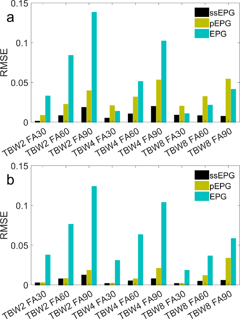
The root-mean-square error (RMSE) of the normalized signals magnitudes modeled by slice-selective (ssEPG), partitioned (pEPG), and conventional EPG without slice profile modeling, relative to the measured signal from the agar phantom over 10 excitations for a crusher strength of one cycle per nominal slice thickness and for four cycles. The time-bandwidth product (TBW) of the Hanning-windowed sinc pulses and the nominal flip angles (FA) in degrees are listed.
The T2 estimates of the MRI system phantom from ssEPG modeling more closely match the ground truth than those from other EPG methods. The plots of T2 estimates over a physiological range of T2 (0 to 100 ms) are shown in Fig. 4a–c. The CCCs in this T2 range are shown in Fig. 4d. Over the full dynamic range, the mean CCCs over all RF pulses and crusher strengths for T1 are 0.994, 0.999, and 0.999 for EPG, pEPG, and ssEPG, respectively; and over the full range of T2s they are 0.919, 0.975, 0.996 for EPG, pEPG, and ssEPG, respectively. As measured by an independent B0 mapping, the ΔB0 of the MRI system phantom contrast inserts did not deviate more than 6.6 Hz, using the mean ΔB0 for each insert.
Fig. 4.

The MRF T2 estimates over a physiological range in the MRI system phantom and concordance correlation coefficients (CCC) from different slice profile modeling techniques for different RF time- bandwidth products (TBW) and crusher cycles per nominal slice thickness (C). The EPG without slice profile corrections are shown in (a), the partitioned EPG (pEPG) results in (b), and the slice-selective EPG (ssEPG) estimates in (c). The dotted line is that of perfect concordance. The CCCs are in panel (d) with error bars indicating 95% confidence intervals.
To further compare pEPG and ssEPG T2 estimation under the closest to ideal crushing conditions used in the MR system phantom experiment, the relative difference in T2 when fitting with pEPG using the ssEPG model as signal reference was modeled for a broad range of T1 and T2 combinations for the TBW of four with four crusher cycles, and then compared with the MR system phantom experimental results. Supporting Information Figure S4 shows that differences in T2 when fit by pEPG using the ssEPG signals as reference range from 0 to ~20% and the experimental results roughly match this modeling.
MRF B0 effects and in vivo application
The simulation of B0 effects in the variable TE/fixed TR MRF sequence modeled with ssEPG are shown in Fig. 5. For a fixed TR sequence such as this, there are modulations in the slice profile magnitude and these modulations are periodic in ΔB0 by frequencies of 1/TR. Fig. 5a shows that the slice profile magnitudes of ΔB0 =1/4TR and 1/2TR are equal to 5/(4TR) and 3/(2TR), respectively. The MRF signal magnitudes at these off-resonant frequencies are also modulated (Fig. 5b). These modulations in magnitude also follow the periodicity of the slice profiles. The phase modulations (Fig. 5c) of the MRF signals show monotonic as well as oscillatory behavior. Again assuming the fixed TR MRF sequence, we find that the phase modulations for |ΔB0|≥1/TR, for MRF signal s at excitation n (parameterized by a given T1, T2 and B1+), can be modeled by multiplying the signal with modulo 1/TR frequency by the added complex phase,
| [10] |
where m=TR{ΔB0−[ΔB0 mod (1/TR)]}, so m is an integer. Two examples of using Eq. (10) to construct higher order frequencies can be seen in Fig. 5c, denoted by asterisks. Using Eq. (10), B0 effects for a given T1, T2, and B1+ can be modeled if the signal is known for ≤ΔB0<1/TR.
Fig. 5.

The magnitude of the slice profiles from the second excitation of the MRF sequences for a TBW of four RF pulse and one cycle per nominal slice thickness gradient crusher at the listed ΔB0s (a). The magnitude of the of MRF signals modeled at the listed ΔB0s (b). The slice profiles and signal magnitudes of ΔB0 = 1/4 and 1/2 overlap with 5/4 and 3/2, respectively, in (a) and (b). The phase of the MRF signals are shown in (c). The 5/4* and 3/2* ΔB0 signals were reconstructed from the 1/4 and 1/2 ΔB0 signals, respectively, using Eq. (10). These reconstructed signals overlap with the explicitly calculated 5/4 and 3/2 ΔB0 signals.
The modeled T1 biases from B0 effects were generally small for the fixed TE sequences, but the relative bias increased with ΔB0 values from the variable TE sequence. The maximum magnitude of relative T1 bias for the fixed TE sequences was < 1% for all TBW and crusher strength combinations. For the variable TE sequence, the T1 bias increased steadily with ΔB0. The maximum magnitude of relative T1 bias for the variable TE sequence for all TBW and crusher strength combinations was < 1%, < 1%, 10%, 22%, and 35% for ΔB0 values (in units of 1/TR) of 0, 1/4, 1/2, 5/4, 3/2, respectively.
Substantial T2 bias can be observed at low ΔB0 values for several sequences. The relative bias in T2 from signals with B0 effects fit against ssEPG dictionaries without B0 effects are shown in Fig. 6. The T2 bias for sequences with TBW/2≥Ncrush increases from ΔB0 of 1/(4TR) to 1/(2TR) and decreases from 1/(2TR) to 5/(4TR). Relative to this, the T2 bias is reduced for sequences with TBW/2<Ncrush, where Ncrush is given as C in Fig. 6 for readability. The T2 bias from the fixed TE/fixed TR sequence is equal between steps in ΔB0 of 1/TR. The bias of the variable TE/fixed TR sequence for the three lowest ΔB0 values is generally equal to or less than that from the other sequences. The contributions to the total crusher strength from the slice-selective gradient before the isodelay and added dephasing gradient (calculated using relations given in the Appendix) for each TBW and crusher combination relative to T2 bias are given in Table 1.
Fig. 6.

The mean relative T2 bias from MRF signals modeled with B0 effects, fitted against models without B0 effects for three different MRF sequences and six different time-bandwidth (TBW) and crusher cycles per nominal slice thickness (C) combinations. The mean is across four physiological T1/T2 combinations noted in the text. Error bars represent the standard deviation of the relative bias.
Table 1.
Modeled T2 bias with RF time-bandwidth product and crusher strength
| TBW a | N crush b | N crush,ss c | N crush,g d | Max. Rel. T2 biase |
|---|---|---|---|---|
| 4 | 1 | 2 | −1 | 0.933 |
| 4 | 4 | 2 | 2 | 0.057 |
| 4 | 8 | 2 | 6 | 0.011 |
| 8 | 1 | 4 | −3 | 0.543 |
| 8 | 4 | 4 | 0 | 0.504 |
| 8 | 8 | 4 | 4 | 0.028 |
TBW – time-bandwidth product
Ncrush – number of crusher cycles per nominal slice thickness
Ncrush,ss – number of crusher cycles from slice-select gradient before isodelay
Ncrush,g – number of crusher cycles from dephasing gradient
Maximum relative T2 bias from fixed TR/fixed TE MRF sequence from the data used in Fig. 6
The parameter maps from the NiCl2-doped phantom and calf using EPG fitting can be seen in Supporting Information Figure S5 and main text Fig. 7, respectively. The T1 maps (Supporting Information Figure S5a, Fig. 7a) of the three different crusher strengths and four different EPG fitting models yield similar results. The EPG T1 estimates without profile effects in the calf muscles appear slightly lower than those from the other EPG modeling. The T2 estimates (Supporting Information Figure S5b, Fig. 7b) are substantially biased using EPG without slice profile effects. The pEPG and ssEPG show drops or abrupt increases in the T2 estimates in the phantom along the B0 gradient, and in the lateral aspects of the calf parameter maps. These deviations are reduced in the maps fit using ssEPG with B0 effects. The mean T1 for the entire non-zero calf parameter maps for EPG, pEPG, ssEPG, and ssEPG with B0 modeling are 1231, 1289, 1290, and 1282 ms, respectively; for T2 they are 63, 22, 24, and 23 ms, respectively. The dictionary generation times for the EPG, pEPG, ssEPG, and ssEPG with B0 modeling are, approximately: 6 min, 58 min, 62 to 316 min (depending on TBW), and 17.4 to 69.1 h (depending on TBW), respectively. Once these dictionaries were computed they could be stored and used repeatedly.
Fig. 7.

The MRF T1 (a) and T2 (b) maps of the calf from three different crusher strengths fit by four different EPG models for a TBW of four RF excitation pulse. The “EPG” fits do not consider slice profile effects. The “pEPG” method accounts for slice profile effects from the RF pulse but idealizes crusher action. The “ssEPG” method accounts for RF pulse and the differences in crusher strength. The T2 of the “EPG” method exceeds the dynamic range of the color mapping, which is reduced to better capture variations in the other fitting models.
Further analysis of the phantom and calf data can be seen in Supporting Information Figure S6 and main text Fig. 8, respectively. The coefficient of variation (COV) of estimated T2 across the different crushers for the different EPG fitting methods (Supporting Information Figure S6a, Fig. 8a) show that ssEPG with B0 modeling has the lowest COV across the different measurements. Regions that are within 30% of the an off-resonance magnitude of 1/(2TR) (Supporting Information Figure S6c, Fig. 8c) correspond to regions of highest COV in ssEPG without B0 modeling. These regions have reduced COV after B0 is considered.
Fig. 8.

The coefficient of variation (COV) of estimated T2 across the different crusher strengths in the calf for the four different fitting methods (a). The mean B0 map in (b) is estimated from the slice-selective EPG (ssEPG) with B0 modeling. An overlay shows regions of ΔB0 that are within 30% of an integer multiple of 1/(TR) from 1/(2TR) (c).
Discussion
Slice profile effects can substantially bias relaxometry estimates in gradient-crushed, free precession sequences. The ssEPG method proposed here accounts for soft RF pulse effects. It also improves on other EPG methods, by accounting for the non-idealized gradient crushing interaction.
The simulation, phantom, and in vivo results demonstrate that ssEPG accurately models slice profiles and associated effects on signal. The simulations with ssEPG indicate that it accurately captures the highly variable magnitudes of slice-selective profiles that result from unbalanced gradients. Such slice profile modulations may be relevant in the context of partial volume effects, and possibly in multicompartment MRF parameter estimation,23,24 depending on the length scale of the heterogeneity of the tissue. The ssEPG model has the lowest RMSE (Fig. 3) and highest CCC (Fig. 4) compared to other EPG methods. The MRI system phantom and in vivo results show that the ssEPG modeling translates to more accurate relaxometry estimates using uSSFP MRF in regions of the |ΔB0| < 7 Hz relative to other EPG-based methods.
The pEPG method markedly reduces RMSE and T2 estimation bias relative to EPG without slice profile considerations, but it is not as accurate as ssEPG over a physiological range of T2. The pEPG RMSE (Fig. 3) and relaxometry estimates (Fig. 4) from the phantom measurements are better than those from EPG without profile modeling. In the steady state (Supporting Information Table S1), pEPG signal is closest to that of ssEPG when two cycles or more of crushing have been completed prior to the commencement of the RF pulse, yet there is still divergence between the pEPG and ssEPG signal models at higher flip angles. The pEPG model in MRF apparently exhibits variable relaxometry bias depending on crusher strength and TBW (Fig. 4). The pEPG model has more variability in T2 across crusher strengths for the given TBW in vivo. Even with the closest to optimal crushing for the MR system phantom experiment, Supporting Information Figure S4 indicates significant differences in T2 estimation between pEPG and ssEPG, suggesting that pEPG T2 estimation bias may be unavoidable in some circumstances.
The effect of ΔB0 on MRF uSSFP T2 relaxometry is substantial and pertains to both fixed and variable TR MRF sequences, whereas the T1 estimates were relatively unbiased by B0 effects. Matching what has been previously reported,12,13 we observe periodicity in the T2 bias at a period of frequency 1/TR, which parallels the modulation of the slice profile over ΔB0. Fig. 6 shows that the T2 bias from the fixed and variable TE MRF sequence are similar at ΔB0 1/(2TR), indicating it is not the phase dispersion of the variable TE causing the bias seen in vivo variable TE/fixed TR MRF T2 maps in Figs. 7–8. Table 1 implies that the source of the T2 bias is insufficient crushing before the slice-select gradient: off-resonance signal components are being transferred by RF action to refocusing and longitudinal states prior to their complete dephasing, later contributing to the net signal. A higher TBW does not reduce this bias, but Table 1 indicates the majority of the T2 bias is eliminated if the transverse magnetization has been dephased more than one cycle per nominal slice thickness prior to the beginning of the next RF pulse. The Appendix details a simple relationship between TBW and crusher strength to ensure sufficient dephasing. Fig. 8 demonstrates that incorporation of B0 into ssEPG reduces the variability of in vivo T2 estimates, particularly in regions of ΔB0 near integer multiples of 1/TR from 1/(TR).
Depending on the crusher strength and TBW, the B0 effects and the MRF contrast effects in a fixed TR MRF sequence are not separable as they are with idealized crushing16,25. However, B0 effects are still separable for higher order frequencies as shown in Eq. (10) and Fig. 5. This separability should be restored for higher crusher strengths and most 3D acquisitions. Yet, in cases where rapid acquisition is required, 3D may not be an option, and diffusion effects26 may limit the use of high crusher strengths.
Limitations of this study are the uncertainty of all sources of influence on in vivo T2 estimates and code optimization. Slice profile effects are only one component that contribute to relaxometry errors. Undersampling effects in MRF have shown to limit the accuracy of MRF.27 Multi-compartment effects, with or without exchange, may bias parameter estimates.28 Notably, a 3D MRF uSSFP study of the brain showed T2 values much lower than those from conventional estimates.29 The skeletal muscle T1 and T2 values in this study are, respectively, consistent with and lower than conventional estimates20. Conversely, the ssEPG T2 estimates in phantom (Fig. 4) are entirely consistent with conventional measurements. Depending on TBW and inclusion of B0 effects, the ssEPG dictionary calculation can be substantially slower than other EPG-based calculation methods. Optimization of the CPU and GPU code is the subject of future work. For example, the number of discrete time steps, NRF, in the ssEPG hard pulse approximation was not optimized in this work. Since the number of ssEPG states scales with NRF (see Appendix), the computation time should scale as , and memory requirements may be decreased by reducing NRF. Reducing NRF may decrease modeling accuracy, but the optimal setting of NRF for a given sequence and desired accuracy is not explored here. Despite these limitations, we have shown: ssEPG provides accurate signal and slice profile calculations, MRF T2 estimation can be improved using ssEPG, gradient crusher interactions with slice-selective excitation may lead to bias that can be corrected with ssEPG modeling, and a simple relationship between TBW and crusher strength can be applied to ameliorate T2 bias in uSSFP MRF without explicit modeling.
While the focus of this work was to apply ssEPG to transient state uSSFP slice profiles, such as those in MRF, this modeling technique could be applied to slice-selective MSE measurements, as well. In situations of low gradient crusher strength or inhomogeneous pulse profiles, ssEPG may yield improvements in T2 estimation. However, further investigation is required to determine ssEPG’s utility in MSE.
In support of reproducible research, the source code along with figure reproduction scripts and data are freely available for download at https://github.com/jostenson/mrm_ssepg (SHA-1: ac87d44).
Conclusions
Transient gradient-crushed sequences such as uSSFP MRF are sensitive to slice profile effects. These profile effects are dependent on RF pulse, crusher strength, and ΔB0. All these effects can be modeled with ssEPG to improve MRF relaxometry estimates as well as to provide insights into the source and relationship of different modes of bias.
Supplementary Material
Supporting Information Note 1. Derivation of Eq. (2) from Eq. (1).
Supporting Information Figure S1. A detailed view of the magnitudes of the simulated, transient slice-profile shapes calculated by numerical solution to the Bloch equations and the slice-selective extended phase graph (ssEPG) techniques from Fig. 1 in the main text. The profiles of repetition (3) and repetition (8) are shown.
Supporting Information Figure S2. A detailed view of the measured and simulated magnitudes of the slice profiles from the agar phantom displayed in Fig. 2 in the main text. The profiles of repetition (3) and repetition (8) are shown.
Supporting Information Figure S3. The ssEPG and pEPG modeled steady state slice profile magnitudes after 100 excitations using the conditions in the agar phantom experiment in the main text. The time bandwidth factor (TBW) and flip angle (FA) are displayed for one cycle of crushing per nominal slice thickness (a) and four cycles (b).
Supporting Information Table S1. The pEPG to ssEPG modeled steady state signal magnitude ratios after 100 excitations using the conditions in the agar phantom experiment in the main text.
Supporting Information Figure S4. The difference in MRF T2 estimation from pEPG and ssEPG modeling for the MRF sequence with a time bandwidth product of four and crusher strength of four cycles per nominal slice thickness. The modeled relative difference in fitted T2 is shown in (a), calculated from the MRF ssEPG signal model fit using the corresponding pEPG dictionary for a broad range of T1 and T2 combinations. The MRF sequence and mean B1+ value from the MR system phantom experiment in the main text was used to generate percentage difference in T2 arising from the ssEPG and pEPG signal model differences that are then interpolated onto a uniform T1-T2 grid. On-resonance was assumed and regions where T1 < T2 have been masked. Overlaid are the ssEPG T1 and T2 estimates from the MR system phantom. These markers correspond to those in (b), which plots the modeled relative difference in pEPG and ssEPG T2 against the experimentally estimated relative difference in T2. The largest deviations between the experimental results and the model (▷, +, ◁) are near regions of high gradients in the difference metric visible in (a). The “+” and “○” are used twice, once in the extreme upper left and again in the lower right of (a), corresponding to the upper right and central position in (b), respectively.
Supporting Information Figure S5. The MRF T1 (a) and T2 (b) maps of the NiCl2-doped phantom from three different crusher strengths fit by four different EPG models for a TBW of four RF excitation pulse. The “EPG” fits do not consider slice profile effects. The “pEPG” method accounts for slice profile effects from the RF pulse but idealizes crusher action. The “ssEPG” method accounts for RF pulse and the differences in crusher strength. The T2 of the “EPG” method exceeds the dynamic range of the color mapping, which is reduced to better capture variations in the other fitting models.
Supporting Information Figure S6. The coefficient of variation (COV) of T2 across the different crusher strengths in the NiCl2-doped phantom for the four different fitting methods (a). The mean B0 map in (b) is estimated from the slice-selective EPG (ssEPG) with B0 modeling. An overlay shows regions of B0 that are within 30% of an integer multiple of from (c).
Acknowledgments
The authors would like to thank: the Vanderbilt University Institute of Imaging Science Human Imaging Core, including Ms. Clair Kurtenbach, Ms. Leslie McIntosh, and Mr. Christopher Thompson for expert technical assistance; Prof. Will Grissom and Prof. Doug Hardin for useful discussions; and Prof. Bennett Landman and Dr. Melissa Hooijmans for assistance in phantom and in vivo measurements.
Funding Sources
NIH R01 DK105371, NIH R01 AR073831, NIH K25 CA176219, NIH R01 EB017230
Appendix
The following is a description of relationships between RF model properties, crusher gradient, and spatial/frequency resolution in ssEPG. The action of off-resonance frequency under free precession in EPG is also noted.
If we define the constant slice-selective gradient strength G, in terms of time-bandwidth product κ, RF pulse approximated in NRF discrete steps of duration τ=NRFΔt, and slice thickness Δsl as
| [A.1] |
and insert this into the definition of Δkz from Eq. (8), we can see that spatial-frequency discretization can also be given as
| [A.2] |
The EPG state matrix is , with Q states, has the effective field-of-view equal to the reciprocal of Eq. (A.2). The discrete spatial-frequency representation of the complex magnetization
| [A.3] |
where , with spacing between states of Δkz and Ω* is the complex conjugate of Ω. For a given resolution in the spatial domain Δz, using Eq. (A.2), Q can be given as
| [A.4] |
A gradient crusher may be applied to Ω, shifting its transverse states by multiples of Δkz. If Ncrush is the number of crusher cycles per nominal slice thickness, and fr is the fraction of the RF duration before the isodelay, then the number of discrete steps applied by the gradient crusher Ncycle is
| [A.5] |
Combining Eqs. (A.2) and (A.5) we can write
| [A.6] |
The net number of discrete steps, ΔN, taken in a time TR from the gradient crusher and the portion of slice-select gradient before the isodelay is given by
| [A.7] |
From this expression and Eq. (A.4) we can write the number of ssEPG states relative to the net shift in state-space over each TR as
| [A.8] |
From Eqs. (A.5–A.7), Ncycle comes from the slice-select and separate dephasing gradient contributions. The number of cycles per nominal slice thickness advanced by the slice-select gradient, Ncrush,ss, is frκ. The remainder from the dephasing gradient is Ncrush,g=Ncrush–Ncrush,ss. So, for fr=1/2, there will be at least one cycle of dephasing prior to RF excitation for
| [A.9] |
Under free precession, complex transverse magnetization M± at position z experiencing an off-resonance of frequency ΔB0 for a time τ can be written as
| [A.10] |
By taking the Fourier transform of Eq (A.9) and assuming that B0 is independent of z, we can write
| [A.11] |
References
- 1.Jiang Y, Ma D, Seiberlich N, Gulani V, Griswold MA. MR fingerprinting using fast imaging with steady state precession (FISP) with spiral readout. Magn Reson Med. 2015;74(6):1621–1631. doi: 10.1002/mrm.25559 [DOI] [PMC free article] [PubMed] [Google Scholar]
- 2.Weigel M Extended phase graphs: Dephasing, RF pulses, and echoes - Pure and simple. J Magn Reson Imaging. 2015;41(2):266–295. doi: 10.1002/jmri.24619 [DOI] [PubMed] [Google Scholar]
- 3.Malik SJ, Sbrizzi A, Hoogduin JM, Hajnal JV. Equivalence of EPG and Isochromat-Based Simulation of MR Signals. In: Proc Intl Soc Mag Reson Med.; 2016:3196. [Google Scholar]
- 4.Lebel RM, Wilman AH. Transverse relaxometry with stimulated echo compensation. Magn Reson Med. 2010;64(4):1005–1014. doi: 10.1002/mrm.22487 [DOI] [PubMed] [Google Scholar]
- 5.Malik SJ, Padormo F, Price AN, Hajnal JV. Spatially resolved extended phase graphs: Modeling and design of multipulse sequences with parallel transmission. Magn Reson Med. 2012;68(5):1481–1494. doi: 10.1002/mrm.24153 [DOI] [PubMed] [Google Scholar]
- 6.McPhee KC, Wilman AH. Transverse relaxation and flip angle mapping: Evaluation of simultaneous and independent methods using multiple spin echoes. Magn Reson Med. 2017;77(5):2057–2065. doi: 10.1002/mrm.26285 [DOI] [PubMed] [Google Scholar]
- 7.Buonincontri G, Sawiak SJ. MR fingerprinting with simultaneous B1 estimation. Magn Reson Med. 2015;00:1–9. doi: 10.1002/mrm.26009 [DOI] [PMC free article] [PubMed] [Google Scholar]
- 8.Cloos MA, Knoll F, Zhao T, et al. Multiparametric imaging with heterogeneous radiofrequency fields. Nat Commun. 2016;7:12445. doi: 10.1038/ncomms12445 [DOI] [PMC free article] [PubMed] [Google Scholar]
- 9.Jaubert O, Cruz G, Bustin A, et al. Water–fat Dixon cardiac magnetic resonance fingerprinting. Magn Reson Med. 2020;83(6):2107–2123. doi: 10.1002/mrm.28070 [DOI] [PMC free article] [PubMed] [Google Scholar]
- 10.Hong T, Han D, Kim MO, Kim DH. RF slice profile effects in magnetic resonance fingerprinting. Magn Reson Imaging. 2016;41:73–79. doi: 10.1016/j.mri.2017.04.001 [DOI] [PubMed] [Google Scholar]
- 11.Ma D, Coppo S, Chen Y, et al. Slice profile and B 1 corrections in 2D magnetic resonance fingerprinting. Magn Reson Med. 2017;78(5):1781–1789. doi: 10.1002/mrm.26580 [DOI] [PMC free article] [PubMed] [Google Scholar]
- 12.Guzek B, Körzdörfer G, Mathias N, Pfeuffer J. Influence of Off-Resonance on FISP Magnetic Resonance Fingerprinting (FISP-MRF). In: Proceedings of the Joint Annual Meeting ISMRM-ESMRMB, Paris, France.; 2018:4264. [Google Scholar]
- 13.Körzdörfer G, Guzek B, Jiang Y, et al. Description of the off-resonance dependency in slice-selective FISP MRF. In: Proceedings of the Joint Annual Meeting ISMRM-ESMRMB, Paris, France.; 2018:4232. http://indexsmart.mirasmart.com/ISMRM2018/PDFfiles/4232.html. [Google Scholar]
- 14.Bain AD, Anand CK, Nie Z. Exact solution to the Bloch equations and application to the Hahn echo. J Magn Reson. 2010;206(2):227–240. doi: 10.1016/j.jmr.2010.07.012 [DOI] [PubMed] [Google Scholar]
- 15.Keenan KE, Stupic KF, Boss MA, et al. Multi-site, multi-vendor comparison of T1 measurement using ISMRM/NIST system phantom. In: Proc Intl Soc Mag Reson Med.; 2016:3290. [Google Scholar]
- 16.Ostenson J, Damon BM, Welch EB. MR fingerprinting with simultaneous T1, T2, and fat signal fraction estimation with integrated B0 correction reduces bias in water T1 and T2 estimates. Magn Reson Imaging. 2019;60:7–19. doi: 10.1016/j.mri.2019.03.017 [DOI] [PMC free article] [PubMed] [Google Scholar]
- 17.Jankiewicz M, Gore JC, Grissom WA. Improved encoding pulses for Bloch-Siegert B 1 + mapping. J Magn Reson. 2013;226:79–87. doi: 10.1016/j.jmr.2012.11.004 [DOI] [PMC free article] [PubMed] [Google Scholar]
- 18.Crawford SB, Kosinski AS, Lin HM, Williamson JM, Barnhart HX. Computer programs for the concordance correlation coefficient. Comput Methods Programs Biomed. 2007;88(1):62–74. doi: 10.1016/j.cmpb.2007.07.003 [DOI] [PubMed] [Google Scholar]
- 19.Wang D, Ostenson J, Smith DS. snapMRF: GPU-accelerated magnetic resonance fingerprinting dictionary generation and matching using extended phase graphs. Magn Reson Imaging. November2019. doi: 10.1016/j.mri.2019.11.015 [DOI] [PMC free article] [PubMed] [Google Scholar]
- 20.Bojorquez JZ, Bricq S, Acquitter C, Brunotte F, Walker PM, Lalande A. What are normal relaxation times of tissues at 3 T? Magn Reson Imaging. 2017;35:69–80. doi: 10.1016/j.mri.2016.08.021 [DOI] [PubMed] [Google Scholar]
- 21.Uecker M, Tamir JI. BART: version 0.4.02 (Version v0.4.02). 2017. doi: 10.5281/zenodo.1066014 [DOI]
- 22.Zwart NR, Johnson KO, Pipe JG. Efficient sample density estimation by combining gridding and an optimized kernel. Magn Reson Med. 2012;67(3):701–710. doi: 10.1002/mrm.23041 [DOI] [PubMed] [Google Scholar]
- 23.Mcgivney D, Deshmane A, Jiang Y, et al. Bayesian Estimation of Multicomponent Relaxation Parameters in Magnetic Resonance Fingerprinting. 2018;170:159–170. doi: 10.1002/mrm.27017 [DOI] [PMC free article] [PubMed] [Google Scholar]
- 24.Nagtegaal M, Koken P, Amthor T, Doneva M. Fast multi-component analysis using a joint sparsity constraint for MR fingerprinting. Magn Reson Med. 2019;(July):mrm.27947. doi: 10.1002/mrm.27947 [DOI] [PMC free article] [PubMed] [Google Scholar]
- 25.Flassbeck S, Schmidt S, Breithaupt M, Bachert P, Ladd ME, Schmitter S. On the In fl uence of Intra-Voxel Dephasing in FISP-MRF with Variable Repetition Time. Proc Intl Soc Mag Reson Med. 2017:1492. [Google Scholar]
- 26.Kobayashi Y, Terada Y. Diffusion-weighting Caused by Spoiler Gradients in the Fast Imaging with Steady-state Precession Sequence May Lead to Inaccurate T2 Measurements in MR Fingerprinting. Magn Reson Med Sci. 2018:1–9. doi: 10.2463/mrms.tn.2018-0027 [DOI] [PMC free article] [PubMed] [Google Scholar]
- 27.Stolk CC, Sbrizzi A. Understanding the Combined Effect of k-Space Undersampling and Transient States Excitation in MR Fingerprinting Reconstructions. IEEE Trans Med Imaging. 2019;38(10):2445–2455. doi: 10.1109/TMI.2019.2900585 [DOI] [PubMed] [Google Scholar]
- 28.Does MD. Inferring brain tissue composition and microstructure via MR relaxometry. Neuroimage. 2018;182(December 2017):136–148. doi: 10.1016/j.neuroimage.2017.12.087 [DOI] [PMC free article] [PubMed] [Google Scholar]
- 29.Ma D, Jiang Y, Chen Y, et al. Fast 3D magnetic resonance fingerprinting for a whole-brain coverage. Magn Reson Med. 2018;79(4):2190–2197. doi: 10.1002/mrm.26886 [DOI] [PMC free article] [PubMed] [Google Scholar]
Associated Data
This section collects any data citations, data availability statements, or supplementary materials included in this article.
Supplementary Materials
Supporting Information Note 1. Derivation of Eq. (2) from Eq. (1).
Supporting Information Figure S1. A detailed view of the magnitudes of the simulated, transient slice-profile shapes calculated by numerical solution to the Bloch equations and the slice-selective extended phase graph (ssEPG) techniques from Fig. 1 in the main text. The profiles of repetition (3) and repetition (8) are shown.
Supporting Information Figure S2. A detailed view of the measured and simulated magnitudes of the slice profiles from the agar phantom displayed in Fig. 2 in the main text. The profiles of repetition (3) and repetition (8) are shown.
Supporting Information Figure S3. The ssEPG and pEPG modeled steady state slice profile magnitudes after 100 excitations using the conditions in the agar phantom experiment in the main text. The time bandwidth factor (TBW) and flip angle (FA) are displayed for one cycle of crushing per nominal slice thickness (a) and four cycles (b).
Supporting Information Table S1. The pEPG to ssEPG modeled steady state signal magnitude ratios after 100 excitations using the conditions in the agar phantom experiment in the main text.
Supporting Information Figure S4. The difference in MRF T2 estimation from pEPG and ssEPG modeling for the MRF sequence with a time bandwidth product of four and crusher strength of four cycles per nominal slice thickness. The modeled relative difference in fitted T2 is shown in (a), calculated from the MRF ssEPG signal model fit using the corresponding pEPG dictionary for a broad range of T1 and T2 combinations. The MRF sequence and mean B1+ value from the MR system phantom experiment in the main text was used to generate percentage difference in T2 arising from the ssEPG and pEPG signal model differences that are then interpolated onto a uniform T1-T2 grid. On-resonance was assumed and regions where T1 < T2 have been masked. Overlaid are the ssEPG T1 and T2 estimates from the MR system phantom. These markers correspond to those in (b), which plots the modeled relative difference in pEPG and ssEPG T2 against the experimentally estimated relative difference in T2. The largest deviations between the experimental results and the model (▷, +, ◁) are near regions of high gradients in the difference metric visible in (a). The “+” and “○” are used twice, once in the extreme upper left and again in the lower right of (a), corresponding to the upper right and central position in (b), respectively.
Supporting Information Figure S5. The MRF T1 (a) and T2 (b) maps of the NiCl2-doped phantom from three different crusher strengths fit by four different EPG models for a TBW of four RF excitation pulse. The “EPG” fits do not consider slice profile effects. The “pEPG” method accounts for slice profile effects from the RF pulse but idealizes crusher action. The “ssEPG” method accounts for RF pulse and the differences in crusher strength. The T2 of the “EPG” method exceeds the dynamic range of the color mapping, which is reduced to better capture variations in the other fitting models.
Supporting Information Figure S6. The coefficient of variation (COV) of T2 across the different crusher strengths in the NiCl2-doped phantom for the four different fitting methods (a). The mean B0 map in (b) is estimated from the slice-selective EPG (ssEPG) with B0 modeling. An overlay shows regions of B0 that are within 30% of an integer multiple of from (c).