Characterizing methane and total non-methane hydrocarbon levels in Los Angeles communities with oil and gas facilities using air quality monitors

Abstract

Over the past decade, sensor networks have been proven valuable to assess air quality on highly localized scales. Here we leverage innovative sensors to characterize gaseous pollutants in a complex urban environment and evaluate differences in air quality in three different Los Angeles neighborhoods where oil and gas activity is present. We deployed monitors across urban neighborhoods in South Los Angles adjacent to oil and gas facilities with varying levels of production. Using low-cost sensors built in-house, we measured methane, total non-methane hydrocarbons (TNMHCs), carbon monoxide, and carbon dioxide during three deployment campaigns over four years. The multi-sensor linear regression calibration model developed to quantify methane and TNMHCs offers up to 16% improvement in coefficient of determination and up to a 22% reduction in root mean square error for the most recent dataset as compared to previous models. The deployment results demonstrate that airborne methane concentrations are higher within a 500 m radius of three urban oil and gas facilities, as well as near a natural gas distribution pipeline, likely a result of proximity to sources. While there are numerous additional sources of TNMHCs in complex urban environments, some sites appear to be larger emitters than others. Significant methane emissions were also measured at an idle site, suggesting that fugitive emissions may still occur even if production is ceased. Episodic spikes of both compounds suggested an association with oil and gas activities, demonstrating how sensor networks can be used to elucidate community-scale sources and differences in air quality moving forward.

Graphical Abstract:

Air quality monitors were deployed in three Los Angeles neighborhoods characterized by oil and gas activity (top); methane levels (bottom left) and baseline removed methane spikes (bottom right) varied based on proximity to oil and gas facilities.

1. Introduction

1.1. Background and Motivation

The growth of oil and gas production in close proximity to communities has driven concerns about impacts to health and the environment. Air pollution associated with oil and gas extraction is a growing concern for public health and environmental quality. Of the chemicals identified in natural gas production, the majority were found to affect the respiratory and gastrointestinal systems as well as sensory organs, and are thought to have long term health effects that have yet to be fully determined (Colburn et al., 2011). Adverse birth outcomes and congenital heart defects have also been associated with pregnant mothers living nearby natural gas and oil development (McKenzie et al., 2014; Tran et al., 2020; Cushing et al., 2020). Numerous studies also suggest that higher rates of immunological deficiencies in adults and children alike may be linked to air pollution from oil and gas activities (Johnston et al., 2019; Yermukhanova et al., 2017; Dey et al., 2015; Kudabayeva et al., 2014; Dahlgren et al., 2007; Willis et al., 2020).

Methane (CH4) and total non-methane hydrocarbons (TNMHCs) are among the direct and fugitive emissions of highest concern at oil and gas facilities, emanating from production, collection, and processing activities (Allen, 2013). Human exposure to high levels of methane can result in nausea, vomiting, headaches, and dizziness (U.S. National Library of Medicine, 2019). Although not all TNMHCs are dangerous to human health, many associated with oil and gas activities can pose serious complications when inhaled (Adgate et al., 2014). More generalized symptoms of exposure may include eye irritation, headaches, and worsening instances of asthma. Many of the aromatic hydrocarbons associated with petroleum production, including benzene, have been linked to cases of leukemia, anemia, and non-Hodgkins lymphoma, among other blood disorders (Adgate et al., 2014; Glass et al., 2003; Kirkeleit et al., 2008; Brosselin et al., 2009; White et al., 2009; Goldstein et al., 2010).

In densely populated urban environments such as Los Angeles, California, the complexity of the surrounding environment also makes determining pollutant sources more difficult. Hopkins et al. concluded that other, often unrepresented, sources of methane in the Los Angeles basin included fugitive emissions from natural gas distribution pipelines, natural gas-fueled vehicles, and waste disposal. In addition, a myriad of industrial centers in the city such as Los Angeles International Airport, downtown, and the Port of Los Angeles were constructed near or directly above major oil fields, making it more difficult to discern anthropogenic sources from their geological counterparts (Hopkins et al., 2016). Nonetheless, the proximity of residents to the epicenters of oil and gas activities raises their exposure risk greatly (McKenzie et al., 2018). In the City of Los Angeles, 70 percent of active wells operate within 500 m of a home or sensitive land use area, including schools and hospitals. Over half a million people live within this radius of an oil and gas facility in Los Angeles alone (Liberty Hill Foundation, 2015). Understanding air quality impacts at a neighborhood scale is important to assess potential health risks.

1.2. Previous Sensor Network Studies in Complex Urban Environments

Over the past decade, advances in air quality monitoring tools and quantification methods have made it possible to deploy a network of sensors in areas of environmental interest, allowing researchers to discern differences in air quality on much smaller spatial scales. The main roadblocks to broader application of these networks, which tend to be made up of less expensive and therefore less accurate tools, are data quality and detection limit. By distributing multiple sensors in complex urban environments, source attribution is possible. Recently, an air quality monitor network in an Italian city showed elevated levels of CO and NOx and worsened overall Air Quality Index (AQI) values near heavily trafficked roadways as opposed to smaller roadways (Brienza et al., 2018). Another network of sensors deployed at and around the London Heathrow Airport successfully apportioned higher CO emissions at sites known to be in areas of more direct aircraft emissions, and elevated NO2 near roadways (Popoola et al., 2018). In the San Francisco Bay area, another monitoring network found the highest mixing ratios of NO, NO2, and ozone among sensors located near an oil refinery. Similarly, sensors near major roadways with diesel traffic read heightened CO and NOx emissions (Kim et al., 2018). A particulate matter sensor deployed on a rooftop and near a freeway in Atlanta, Georgia, and later in Hyderabad, India, showed the highest levels of particulate matter in the more polluted city (Hyderabad), with elevated concentrations near a freeway in Atlanta as opposed to on a rooftop (Johnson et al., 2018). Many other previous studies in urban environments similarly have focused on incomplete combustion products such as CO and NO2. Here we focus on organic gas phase species, specifically methane and total non-methane hydrocarbons. While methane is mainly associated with oil and gas in the area of interest, TNMHCs may emanate from a wide variety of sources.

In southern California, regulatory agencies are deploying suites of sensors to inform residents of air quality on a more localized scale than ever before. South Coast Air Quality Management District (SCAQMD), which encompasses all of Los Angeles County in its jurisdiction, is the government agency responsible for regulating and monitoring emissions in each of the neighborhoods studied (AQMD, 2019). SCAQMD deployed approximately 400 commercially available sensors in California communities over a five-year period, evaluating the sensor models used through the Air Quality Sensor Performance Evaluation Center, and making their results and recommendations publicly available (Collier-Oxandale et al., 2020). However, the focus for most of these deployments was on particulate matter as opposed to gas-phase pollutants. In addition, none of these deployments occurred in or around any of the South LA neighborhoods discussed here.

The Hannigan Lab at the University of Colorado Boulder has used the Y-Pod multi-sensor platform (“pods”) to examine community-scale air quality in southern California. Approximately 90 kilometers east of Los Angeles, a Y-Pod sensor network was deployed in Riverside, CA in 2015. Researchers distributed the pods across a 200 square kilometer area, finding that differences in pollutant levels could be observed on both regional and neighborhood scales (Sadighi et al.,2018).

Y-Pod sensor network studies have taken place directly in Los Angeles. In the fall of 2016, Collier-Oxandale et al. (2018a) began assessing best practices for deploying sensors in complex urban environments, as well as co-location and calibration techniques. Focusing on methane specifically, this work developed methods to filter out improbable sensor and reference readings to improve calibration fits and applications to field data. This prior research also explored sensors’ cross-sensitivities to environmental factors as well as other pollutants (e.g., CO), demonstrating that inexpensive volatile organic compound (VOC) sensors can provide useful information on ambient methane in urban environments. (Collier-Oxandale et al., 2018a). This data was also mapped to potential sources and individual air quality events observed throughout the community as reported by residents (Collier-Oxandale et al., 2019).

In the North University Park neighborhood of Los Angeles, Y-Pods were once again deployed throughout the neighborhood to determine air quality differences on a small spatial and temporal scale from November 2016 to June 2017. This also included deploying five pods on different locations on the same building to determine micro-climate effects, suggesting that a myriad of pollutant sources exist in the area even on a highly localized scale in such a densely populated urban environment (Collier-Oxandale et al., 2018b). A diurnal trend of elevated nighttime concentrations and lower daytime concentrations was observed for CH4 and TNMHCs alike.

Both neighborhoods were chosen as a result of interest from local residents, driven in large part by proximity to urban oil and gas facilities. While oil and gas activities were ongoing in the West Adams neighborhood, active production at the site in North University Park had ceased. A comparison of sensor readings in each neighborhood showed not only elevated baseline CH4 concentrations in West Adams, but also more episodic spikes related to oil and gas activities (Shamasunder et al., 2018).

This study is a continuation of the previous studies in oil-adjacent communities in South Los Angeles. The preliminary results of these first two studies are re-examined using a newly developed calibration model that improves sensor fits; this is discussed in section 3.1. In addition, another active oil facility was monitored throughout 2019, allowing us to examine trends among multiple oil and gas facilities in Los Angeles in a more extensive comparison than has been presented previously. All three facilities draw from the Las Cienagas oil field; their production outputs should have similar chemical properties (LA City Planning, 2016). This multi-year study of highly localized gas phase pollutants in Los Angeles, specifically with respect to urban oil drilling, is among the first and most exhaustive of its kind to date.

1.3. Study Site Demographics

To better characterize the neighborhoods and understand the environmental justice implications of oil and gas activities in these communities, demographics reported by the California Census Bureau are included. The median values of the 3–4 nearest census block groups to each facility, consisting of a few city blocks each, are considered and should provide insight as to which income brackets and racial or ethnic groups are most affected by neighborhood oil and gas activities. Note that this data was collected from 2013–2018 by the American Community Survey, California Public Utilities Commission, and the Planning Database.

In the area surrounding the Deployment 1 site, 56% of residents identified as Hispanic or Latino, 29% Black, and 10% Asian. 51% of the community was below 150% of the poverty line. In Deployment 2’s neighborhood, 47% identified as Hispanic or Latino and 12% as Black, with 59% below 150% of the poverty line. For the Deployment 3 area, 43% identified as Hispanic/Latino while 47% identified as Black. Similarly to the other two neighborhoods, 54% self-reported as their annual household income being below the 150% poverty line.

In terms of land use, for each deployment most of the area within 500 m of the oil and gas facility is residential and prone to overcrowding. Educational (institutional) and public land use (miscellaneous) claim the next largest proportion of area, including schools, preschools, and libraries. Little to no land is unused in any of these 500 m circles (Liberty Hill Foundation, 2015). This land use data is shown in Figure 2-C.

Figure 2.

A) Colocation locations, with color indicating which study/studies each reference instrument was used for; B) Sensor deployment locations for all three studies, with the oil and gas facilities and surrounding 500 m radius indicated; C) Land usage within each 500 m radius.

2. Methods

2.1. Overview

We followed the sensor field normalization and deployment methodology set forth by previous studies (Piedrahita et al., 2014; Clements et al., 2017; Collier-Oxandale et al., 2018a; Sadighi et al., 2018; Casey et al., 2019; Vikram et al., 2019). The sensor packages used were run adjacent to a high-quality reference monitor, operating under similar conditions to those anticipated during the deployment. The reference data was treated as the standard, and linear regression was used to fit the raw sensor readings to the reference value in parts per million (ppm) for each pollutant. We then deployed our sensor packages in the neighborhoods surrounding three urban oil and gas facilities in South Los Angeles, and applied the calibration models developed previously to the data collected in the field.

2.2. Deployment

We deployed Y-Pods, our embedded sensor packages, in three South Los Angeles neighborhoods from 2016 to 2019. More information on the pod configuration is provided in section 2.3. Three oil and gas production sites, within three km of each other, were selected as the focal points for three deployments. For each deployment, 4–11 pods were placed within a 500 m radius of the production site, and 2–11 were placed outside the 500 m radius. This included sites adjacent to freeways, a major source of hydrocarbons and combustion products. This also included control sites, that is, areas upwind of oil operations and away from any obvious hydrocarbon sources.

While the number of active wells at the two sites with verified ongoing operations were identical (see Supplemental Table S1), the facility studied in Deployment 3 had the highest oil production while Deployment 1 had the highest gas production in 2017 (California Department of Conservation, 2019). Deployment 2 ceased operations in November 2013 after an Environmental Protection Agency investigation, and was subsequently ordered to pay 1.5 million dollars in penalties and address onsite equipment failures and leaks (Southern California Public Radio, 2016).

Due to community and reference instrument constraints, each of the studies took place during different times of year and lasted different amounts of time. The timeline provided in Figure 1 details deployment information.

Figure 1.

Colocation and deployment timeline. The colored bars indicate which compounds were field normalized at each time, while the pink bars indicate the sensor packages being deployed in the neighborhoods.

2.3. Instrumentation – Low-Cost Air Quality Monitors

In each deployment, low-cost air quality monitors dubbed Y-Pods were used for data collection. Their specifications and a list of environmental and gas-phase sensors employed in each is described in detail by Collier-Oxandale and colleagues (Collier-Oxandale et al., 2018a). Briefly, a suite of metal oxide sensors is used to assess hydrocarbons, an NDIR sensor monitors CO2, and an electrochemical sensor measures CO. Each Y-Pod is also equipped with internal temperature and humidity sensors, and all data is stored locally. Unlike reference-grade air quality monitors, which can cost tens of thousands of dollars, each pod is made up of commercially available sensors and cost approximately $1,000 to produce. Thus, for the same cost as one instrument, tens of Y-Pods can be deployed, informing us of air quality differences on more highly localized spatial and temporal scales.

Due to their small size and relatively simple power requirements, the Y-Pods can be placed in strategic locations throughout the communities of interest. Community members were actively involved in the siting process, volunteering their properties to serve as pod locations and ensuring the placements would not obstruct their day-to-day activities. Common Y-Pod siting constraints included safety, access to wall power, sufficient airflow, and likelihood of pods being unplugged or otherwise tampered with. Homes with air pollutant sources such as smoking or barbeques were avoided. Many were placed on single to multi-story roofs of homes and churches; others were placed on top of residential sheds and garages. In each of the deployments discussed, pod placements were determined collaboratively between researchers and the involved individuals as to preserve the integrity of the study without compromising the functionality of the space.

2.4. Sensor Calibration, Validation, and Analysis

To field normalize or calibrate, the sensors were co-located with regulatory grade air quality monitors for approximately one to two weeks at a time. Linear regression was then used to fit the sensor data to the regulatory data. One of the main advantages of this approach is that the sensors are calibrated using the same range of temperatures, humidities, pressures, and pollutant concentrations that they are exposed to throughout the field campaign (Collier-Oxandale et al., 2018a).

In previous publications involving the Figaro metal oxide sensors, a clean air normalization factor was utilized; the raw signal values from the sensors were all divided by the lowest value recorded, representing the cleanest air experienced, prior to calibration (Collier-Oxandale et al., 2018a; Collier-Oxandale et al., 2018b; Eugster et al., 2012). In this study, the raw sensor signals were used alone rather than normalizing. When this approach was tested, calibration and validation coefficients of determination did not improve for every pod calibration, and those that improved did so by less than 1%. We hypothesize that this clean air normalization may be more important for studies with wider temperature and humidity ranges than those observed in Los Angeles.

Due to the limited availability of reference pollutants at each colocation site, and some reference instruments being moved during longer deployments, several reference sites were used for each deployment. For deployment 3, pre and mid colocations were not available at most sites due to reference instrument failures. Descriptions of the reference instruments are presented in Supplemental Table S2.

The pods were co-located at each reference site associated with each deployment, but due to occasional power supply issues not every pod recorded sufficient data at every site. Calibration models specific to each pod were used for the following analysis.

For the first study (Deployment 1), as previously described in Collier-Oxandale et. al. (2018a), the pre-deployment colocation took place on a trailer in an open field. Pods were placed 0.75 – 1.5 m off the ground on the side of the trailer nearest the inlet. For the post-deployment colocation in Los Angeles, pods were mounted to a railing approximately 1–2 m above the roof of the building the reference instruments were housed in, about 10 m away from and 1–2 m below the inlet. While some pollutant spikes seen by the samplers may not have been picked up by the pods due to the distances between them, the best possible configurations within the limitations of the activities at the sites were chosen. The additional colocation data collected for Deployment 1 followed the same procedure as that of the following deployments.

During the Deployment 2 and 3 colocation periods, the Y-Pods were stacked two across on top of an approximately 0.5 m high plastic container directly on the rooftop within 1–1.5 m of the reference instrument inlet. While the TNMHC site was a two-story rooftop, the rest of the samplers were on one-story roofs of trailers. The Deployment 3 study was originally intended to be a seven month long deployment, but due to reference instrument failures during the pre and mid deployment calibrations, only the second half of the deployment data was utilized. Each of these sites was operated by either South Coast Air Quality Management District or the California Air Resources Board (CARB). Maps detailing the approximate location of each reference site and monitor for each of the studies are shown in Figure 2.

Each deployment took place during different years, and different times of year; thus, a local reference monitor was sought out as a comparison tool. Throughout 2016, the NASA Megacities project deployed Picarro G2301 and G2401 methane, CO, and CO2 monitors on a rooftop on the USC campus (Verhulst et al., 2016), closest to the Deployment 2 site and not far from the others. No pods were placed at this precise location. This data, discussed in section 3.6, highlights to what extent variation among deployments was the result of yearly differences rather than the oil and gas facilities themselves.

For each deployment, a randomizing 3-fold algorithm was used to select 2/3rds of the co-location data from which to build the calibration algorithms, and the remaining 1/3rd was used as validation data. By selecting data randomly, we hoped to avoid overfitting and ensure differing environmental parameters throughout the colocations were adequately represented.

Baseline removed (subtracted) concentrations are shown to focus on spikes in the data above the normal boundary layer fluctuations which are likely caused by nearby short duration source emission plumes. This approach was originally described by Heimann et al (2015) and later employed by Collier-Oxandale et al. (2018) in South Los Angeles. We will briefly summarize their approach here. The deployment data was split into three-hour intervals, and the 50th percentile of the data in each interval was set as the baseline. This baseline was then smoothed and subtracted from the original field data. This includes the crests of the diurnal patterns as well as larger spikes. An example of ppm-converted data and the resulting baseline removed data from approximately three days of minute average data from the Deployment 3 study can be seen in the supplemental (Figure S1).

2.5. Data Validation

In general, as much reference data as was available for each pollutant was used for calibration and validation. However, for pollutants where multiple reference sites were used to co-locate, this approach proved challenging. Due to differing concentration ranges and multiple reference instruments being used at different sites, it was difficult for the models to fit the different sections of reference data if all the reference data was used for a single model. In general, the more similar the two reference instrument environments, the higher likelihood that the two reference data streams could be integrated into one model. This was an issue for methane throughout the Deployment 2 study, which occurred over a seven month period. A “bookending” method was used to remedy this. The pre-deployment colocation and mid-deployment colocation-data were used to model the first half of deployment only. Likewise, the mid- and post-data were used to model the second half of the deployment. For the Deployment 3 study, multiple reference instrument issues during the mid-deployment colocation made it impossible to model the full deployment without extrapolating; thus, only the second half of the deployment data was utilized.

The data collected by the pods was analyzed to ensure its validity, and periods of time that did not meet data quality checks were ultimately excluded from our analysis. After applying the models described in section 2.4, the R2 comparing each individual pod with the rest of the pods for each pollutant of interest was computed. Those that did not correlate well with the rest were examined more closely for power loss, sensor issues, and calibration inconsistencies for both the colocation and deployment data. The deployment thresholds for validity varied by study wave and pollutant (see Supplemental Table S3). Additionally, different thresholds were chosen for each since the calibration fits differed slightly for each deployment, and some deployments had more control sites outside of the 500 m radius. CH4 and TNMHCs were considered the main pollutants of interest, while CO and CO2 were used to inform the origins of CH4 and TNMHC. All four species concentrations were used to determine which pods overall to include, although only two pods in each deployment had CO sensors, which limited our analysis.

The metal oxide sensors used to quantify methane and TNMHCs are known to deteriorate over time. The linear regression models use different coefficients for each pod for each deployment to help account for this, but by the Deployment 3, some raw signal values were noticeably experiencing “pegging”, where they would record an abnormally large value periodically. Pods that experienced this throughout the duration were not used, while these spikes were removed for pods that only experienced this for a shorter period. Thus, this may have affected data quality and completeness for several of the pods throughout Deployment 3.

2.6. CO2 Sensor Drift correction

In previous studies, the CO2 sensors signals tended to drift over time to a degree that required additional drift correction measures (Collier-Oxandale et al., 2018b). The drift correction method used in this study is summarized as follows. The colocation model was first applied to the pod data. A line was then fit to the converted data, and this line was subtracted out from the fitted pod data. The atmospheric background level of CO2 in Los Angeles, 400 ppm, was then added to this result (Verhulst et al., 2016).

The most recent year of available CO2 reference data, 2016, was used to determine the approximate atmospheric background level for Deployment 2 and Deployment 3. For Deployment 2 specifically, since there was an approximately month-long gap between the fall and spring data due to the mid-deployment colocation, this process was repeated separately for each portion of the deployment. Since the Deployment 1 study was the shortest deployment, the CO2 sensors did not drift significantly and were not corrected.

3. Results

3.1. Calibration Model Results

Based on previous studies (Collier-Oxandale et al., 2018a; Collier-Oxandale et al., 2018b), models that include temperature and humidity perform better than pollutant-specific sensors alone. Using multiple VOC sensors to model methane and TNMHCs has also been demonstrated to be more effective than single sensor models (Collier-Oxandale et al., 2019). In that previous work, the same model form produced the best fit for both methane and TNMHCs.

For Deployment 1 and Deployment 3, the elapsed time term was included to account for sensor drift. For Deployment 2, the longest deployment, this term was not included in the calibration equations for any of the pollutants. While this may seem counterintuitive, the bookending approach for that deployment ensured that for calibrations were only applied to about three months of data at a time. In addition, the Los Angeles region experienced significantly higher rainfall throughout Deployment 2 than during the other two deployments (LA Almanac, 2020). When using the elapsed time term, we hypothesize that it may have partially offset the large humidity value. Thus, the fit was worsened, and the elapsed time term was not included in the final calibration for Deployment 2.

The models for each pollutant included an intercept, temperature term, humidity term, and a term associated with the sensor for the pollutant of interest. For methane and TNMHCs, since there were two hydrocarbon sensors utilized, these both included a term for the light VOC sensor, a term for the heavy VOC sensor, and an interaction term consisting of the light VOC signal divided by the heavy VOC signal. The full models used in each deployment can be found in the supplemental (Table S4).

As shown in Figure 3, changing the multi-sensor term from the product of the two VOC sensors, as done in previous studies, to the ratio of the two, the coefficient of determination (R2) between pod and reference data increased while the root mean square error (RMSE) was reduced. On average, the calibration R2 was 0.692 for Deployment 1, 0.714 for Deployment 2, and 0.799 for Deployment 3. The full results can be found in the supplemental (Table S5, S6).

Figure 3.

Boxplots of Calibration and Validation a) R2 and b) RMSE, grouped by study and pollutant.

The differences in R2 and RMSE among studies can be largely explained by the reference data available. Generally, fits improved when the two book-ended colocations took place at the same reference site. It also helped if that colocation site was close to the deployment region or at least had similar concentrations of the pollutant as the deployment region. For longer colocations, having multiple colocation periods helped to account for sensor drift and seasonal changes in sensor signals.

3.2. Deployment 1 Methane and TNMHCs

Although the data collected in the 2016 deployment has already been analyzed previously (Shamasunder et al., 2018; Collier-Oxandale et al., 2018a), in this section we will re-examine it using the improved calibration models in order to better inform the comparison across the three deployments. Deployment 1 includes the most control sites outside of the 500 m radius of the oil and gas facility; we will focus our analysis on those nearby. Figure 4A shows the baseline removed concentrations at each location throughout this deployment.

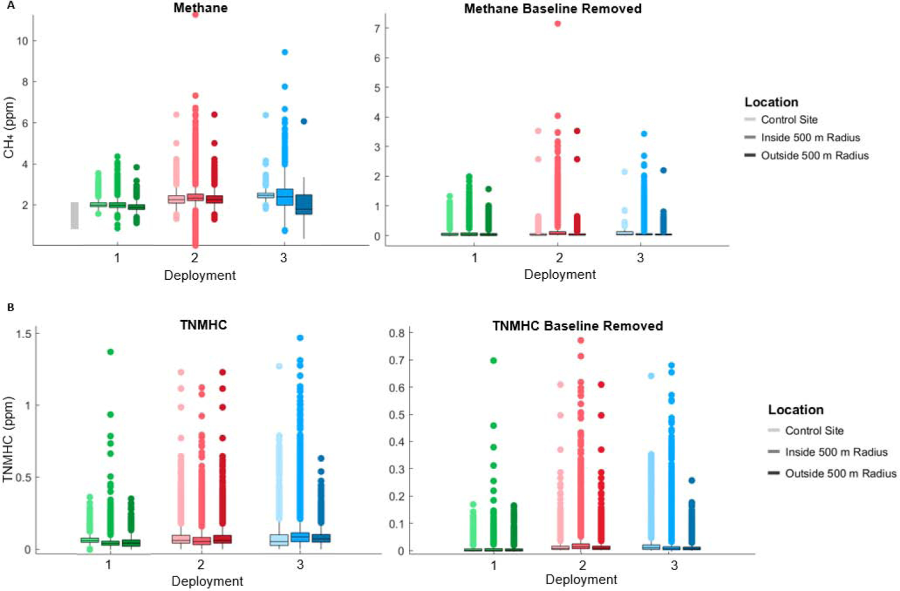
Figure 4.

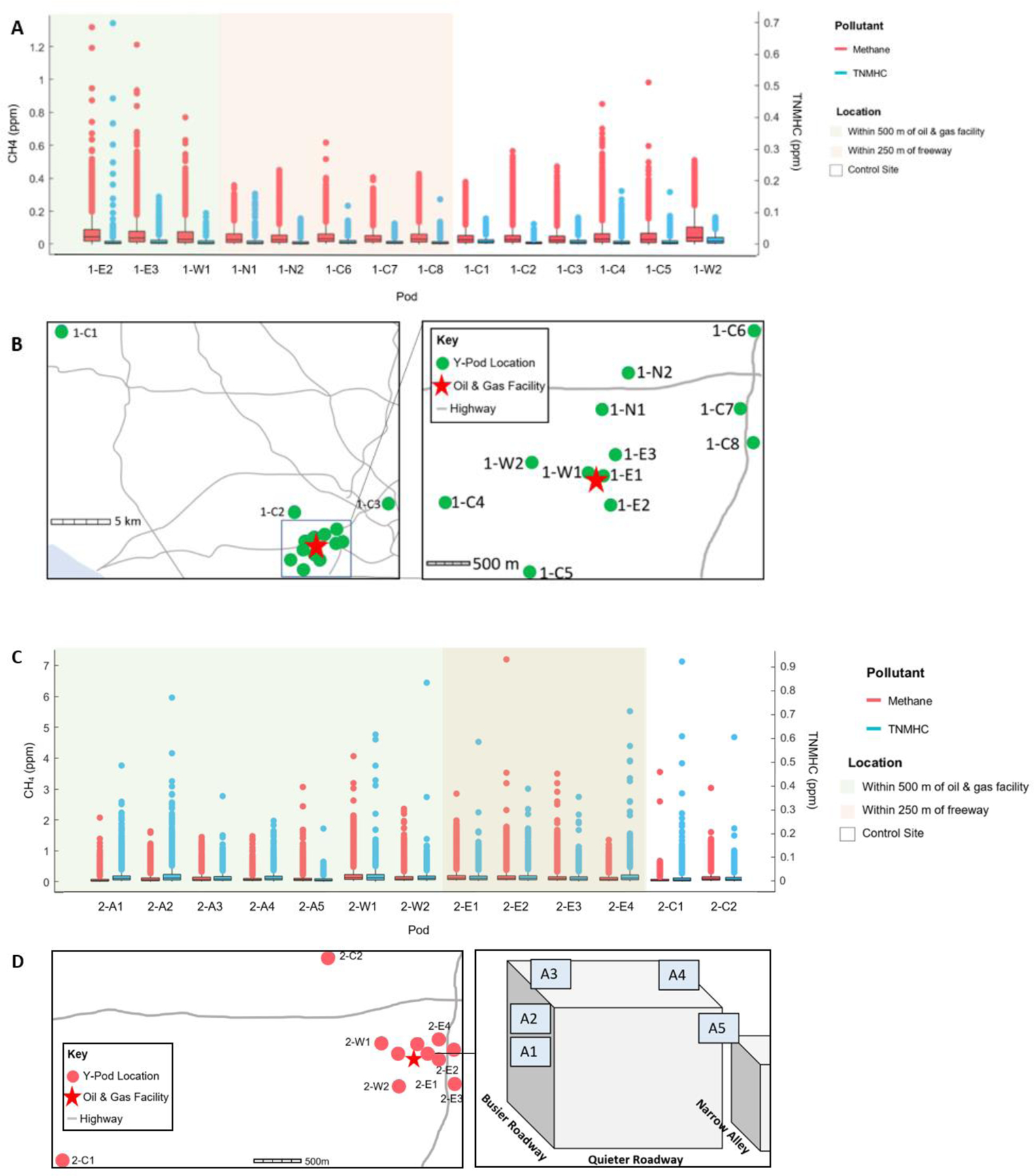
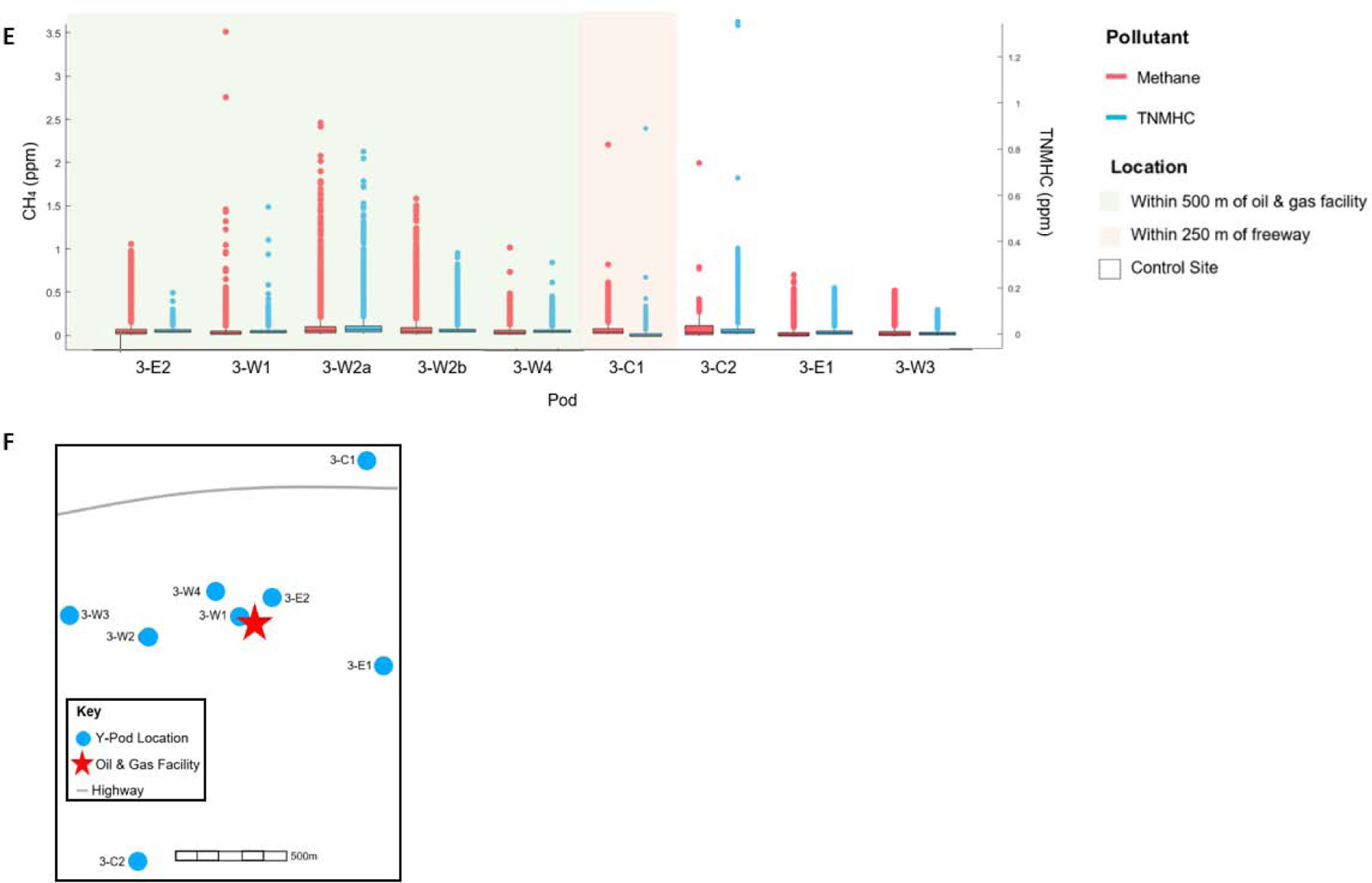
50th Percentile baseline removed boxplots for methane and TNMHCs (top); Monitor locations relative to the oil and gas facility (bottom) for: A-B) Deployment 1; C-D) Deployment 2; E-F) Deployment 3.

1-E1, the only pod located due east of the facility, is not included in this analysis due to excessive power failures and limited recorded data. At the two remaining downwind pods, 1-E2 and 1-E3, methane spikes were the highest. 1-E2 saw the highest TNMHC spikes as well, although it is unclear if this is related to oil and gas activity since 1-E3 saw much more moderate spikes of the same compound. 1-W1, the monitor located closest to the facility albeit slightly west, also registered high spikes of methane but similarly failed to pick up on TNMHCs, further suggesting that methane spikes were related to oil and gas while TNMHC spikes may be another source. The high spikes of both compounds at control site 1-C4 likely has to do with natural gas distribution, discussed in further in section 3.8.

3.3. Deployment 1 Carbon Monoxide

Carbon monoxide sensors were installed in two of the pods used in the study. We will focus on 1-E3, which is within the 500 m radius of the site, rather than 1-C1, located over 30 km from the neighborhood. While CO concentrations measured at this pod are correlated reasonably well with both methane (R2 = 0.706) and TNMHCs (R2 = 0.757), no clear patterns emerged when all three were considered together. This suggests that methane and CO are being co-emitted from the same combustion source, possibly facility related activity, some of the time, while periods of time where TNMHCs and CO are highly correlated are likely due to another combustion source, potentially motor vehicles.

3.4. Deployment 2 Methane & TNMHCs

Although the facility that Deployment 2 focused on was listed as idle at the time of the study, maintenance and other activity was occurring onsite. The baseline subtracted concentrations from this deployment are shown in Figure 4C. For this deployment, more monitors were located downwind and within the 500 m, resulting in higher concentrations on average compared to the other deployments. Most of the high methane spikes are all seen at the monitor locations closest to the oil and gas facility and at downwind sites. We have not been able to locate any other obvious sources in the area, suggesting that emissions are still related to the oil and gas facility. 2-W1, located four blocks upwind of Deployment 2, experienced the largest spikes of methane. Aside from the control site that was used in all three studies which saw elevated concentrations from a separate source, the next highest methane spikes were seen at downwind locations 2-E2 and 2-E3.

For TNMHCs, the trends are not as straightforward since there are generally more sources of TNMHCs in urban regions than methane. Some of the trends we saw for methane spikes hold true for TNMHCs, such as the larger spikes registered nearby and directly east of the site (2-W1 and 2-E4). However, other pods where we saw higher methane spikes, such as 2-E3, did not experience elevated TNMHC levels. Likewise, two of the five monitors located on the same street as the well site, recorded much larger relative spikes in TNMHCs (2-A1, 2-A2). However, the control site used in all three studies, 2-C1, showed the highest TNMHC spikes, demonstrating other local TNMHC sources in the area, as shown in Figure 4C.

3.5. Deployment 2 Carbon Monoxide

CO sensors were integrated in a pod near the freeway approximately two blocks northeast of the facility (2-E4), and in a pod across the street from the facility (2-A3). Even with no active oil and gas operations in the neighborhood, CO still saw significant coefficients of determination with respect to both CH4 and TNMHCs. Since the facility is inactive and we would not expect to see combustion markers emanating from it, the correlations are likely driven by the elevated CO emissions throughout an urban community with high traffic; this may simply prove the prevalence of these compounds across the entire region. However, since the exact scope of activities at the site during this period is unknown, we cannot rule out the possibility of them being linked to other oil and gas activities that may have been ongoing. The neighborhood surrounding Deployment 2 is also east and therefore downwind of the other two nearby active sites, so it could still be affected by oil and gas extraction activity from these upwind sites. These correlation coefficients are listed in Supplemental Table S7; both are reasonably well correlated and suggests that CO emissions may have been emitted from the same source as our pollutants of interest.

3.6. Deployment 3 Methane and TNMHCs

We will similarly focus on the baseline subtracted results for the Deployment 3 site, as shown in Figure 4E. The highest methane spikes were observed at 3-W1, the “fence-line” monitor placed approximately 9 m from the facility. Higher spikes were also observed at 3-W2, two monitors place together approximately two blocks upwind of the oil and gas facility. Proximity of each of these to the facility is thought to be responsible for the larger spikes observed at each of these. Although TNMHC concentrations were moderate for 3-W1, spikes were relatively large for 3-W2.

3-E1 and 3-E2, the two monitors east of the facility, generally saw higher methane spikes than sites further west and control sites, but they tended to be lower than those seen at monitors closest to the site. We believe the relative heights of the monitors may have affected these results. Most monitors were placed on first or second story roofs, while 3-E1 was located on the roof of a shed (approximately 2 m high) and 3-E2 was located on the roof of a seven-story building (approximately 20 m high). Since the vertical placement of these monitors differs greatly from the others, it is possible that each monitor was not exposed to the same plumes from the oil and gas facility, or that the downwind sites may have missed some plumes entirely based on their distance from the ground. 3-E1 appears to have recorded higher concentrations of TNMHCs than other sites, while 3-E2 captured one much higher spike.

At the control site located near the freeway, 3-C1, methane spikes remained relatively moderate, as expected. The other control site, 3-C2, experienced the largest range of spikes overall and a few large spikes. For TNMHCs, we had expected the concentrations to be elevated near the freeway, but were surprised to see the largest spikes at the control site, 3-C2.

Similar temporal patterns for methane and TNMHC spikes were observed at the 3-W2 and 3-W4 locations. Despite being slightly west of Deployment 3, each of these are very close to the site and could represent emissions from oil and gas activity. 3-E1, which was most directly downwind of the site, also shows strong correlations between the two pollutants, furthering this narrative. 3-E2, located on the highest rooftop, showed little correlation, and likely failed to adequately capture plumes from oil and gas activity. Although methane and TNMHCs were not highly correlated at 3-C2, the neighborhood control site, both were elevated for different periods of time. The natural gas pipeline nearby this site also passes through the area where 3-W2 and 3-W4 were located. The high correlations between methane and TNMHC at each of these three sites strongly suggest that the facility is an important source of spikes of both pollutants. Some observed spikes in either compound might still be attributed to the pipeline. We clearly see spikes of both methane and TNMHCs at sites nearest the oil and gas facility especially, although they do not both necessarily occur at the same time and could be emanating from different processes at the facility rather than representing the same emission event every time.

3.7. Methane and TNMHC comparison among the three deployments

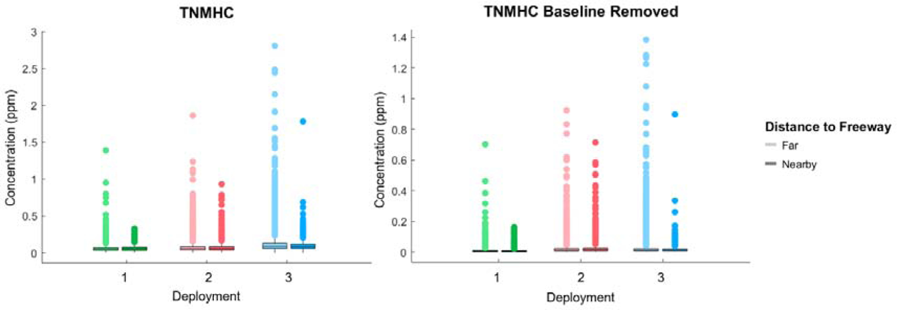
For our neighborhood comparison, the pods were grouped based on whether they were placed within 500 m of the oil and gas facilities or outside of the 500 m radius. We use this 500 m radius as an indicator for impact from emissions from the oil and gas activity. Note that each site had different numbers of pods within their respective 500 m radii: 3 inside and 10 outside (800 m - 8 km away) for Deployment 1, 11 inside and 1 outside (4 km away) for Deployment 2, and 5 inside and 3 outside (800 m – 1 km) for Deployment 3. A control site used throughout all three studies was considered its own category and not included in the outside radius category for any of the sites, which we discuss in section 3.9.

For methane, across all three deployments, we observed higher interquartile ranges and spikes within the 500 m radii than outside, indicating that all three sites are sources of methane in their respective communities. Across the three sites, Deployment 1 had the lowest concentrations overall; this is thought to be the result of the time of year and its respective atmospheric conditions, which are discussed in further detail later in this section. We see the largest range of concentrations at the Deployment 3 site, suggesting that changing concentrations could be correlated with periods of on-site oil and gas activity or maintenance activities. As mentioned in section 3.3, the Deployment 2 oil wells ceased production in late November 2013, however maintenance activity and repairs continued at the site, so methane emissions within the 500 m radius may still related to the facility. This data is shown in Figure 5.

Figure 5.

Regular and baseline removed boxplots of concentrations at the control site, within 500 m of each facility, and outside the 500 m radius for: A) Methane; B) TNMHCs. The highest concentrations and spikes of methane can be seen within the 500 m radius. TNMHC spikes tended to be higher within the radius, although overall concentrations were more mixed.

To better quantify these results, we used a paired t-test to compare hourly averaged data from pods stationed within 500 m of the oil and gas facilities as well as within 250 m of freeways. The p-values of each analysis are listed in Supplemental Table S8. The p-values represent whether the different locations (near a facility, away from a facility; near a freeway, away from a freeway) had significantly different medians. Although most of the individual pod data was not normally distributed, one pod from Deployment 2 (2-C1) was excluded during this analysis as it contributed to tabulation errors.

Although methane concentrations appear to be significantly different based on freeway proximity, this is more likely the result of most pods located near freeways being more than 500 m from an oil and gas facility; this mirrors the statistically significant results in the leftmost column. We would not expect freeways to be a source of methane; we consider this a confounding result based on the distance between the facilities and freeways in the area.

For TNMHCs, the t-test found statistical significance for pods located near freeways for Deployments 1 and 3 only. During Deployment 2, the pods had the least distance among them overall and the most overlap between oil and gas and freeway locations, which may have contributed to the TNMHC results being flipped with respect to the other two deployments. Overall, it appears traffic is an important local source of TNMHCs, while the oil and gas facility is contributing methane.

Both Deployment 1 and Deployment 2 saw modest TNMHC concentration differences comparing the monitors within the 500 m radius compared to monitors farther away, but much higher episodic spikes signified by baseline subtracted data within the 500 m, suggesting that these events may be attributable to the sites themselves. Deployment 3 identified a larger concentration range and higher spikes within the radius as compared to pods further away. Although this could be attributed to activities at the Deployment 3 site, the oil and gas facilities seem to be a less obvious source of TNMHCs as compared to methane.

Building on our ANOVA analysis for TNMHCs, the pods are plotted based whether they were within 250 m of a freeway or highway in Figure 6. From our initial analysis, higher TNMHC concentrations were not observed near major roadways, which is not in line with what we would expect. Although it is worth noting that across all three deployments, only one of the pods located near a freeway was downwind of the prevailing wind direction, so emissions may not have been picked up on as expected.

Figure 6.

A) Regular and B) baseline removed boxplots of TNMHC concentrations within 250 m of a freeway and elsewhere throughout each community.

The location of pods in each community relative to their respective oil and gas facilities may also have influenced these results. In the Los Angeles region, the prevailing wind direction is westerly, blowing inland from the coast (Weather Underground, 2020). However, our ability to examine downwind effects was limited by the monitor placement and data completeness. For Deployment 1, there was only one pod located due east of the facility, and this pod suffered from intermittent power loss and only recorded about two weeks’ worth of data throughout the two month deployment. The pod southeast of the Deployment 3 site was just outside of the 500 m radius. This pod and the northeast pod alike may have additionally been affected by height differences, further discussed in section 3.6. Deployment 2 had the most optimal downwind pod placements, with two sites nearly directly downwind of the site, although we would not expect to see spikes from the facility if it was truly idle. Across all three sites, neither CH4 nor TNMHCs displayed clear trends with respect to temperature, wind direction, month, or time of day.

We also investigated the hourly trends for each of the main compounds to determine how pollutants concentrations in the boundary layer may have changed throughout the day. We used Pacific Standard Time; our values are consistent with meteorology but may vary with human activities such as traffic and hours of oil and gas operation that vary with daylight savings. These diurnal concentration trends are shown in Figure 7. Again, we separate pods based on proximity (control, within 500 m and outside 500 m). We also included data on most of the key pollutants collected at USC, closest to the Deployment 2 neighborhood, by NASA’s Megacities Project throughout 2016. The rightmost graphs show this dataset sorted according to time of year; we show three Megacities diurnal profiles, each corresponding to the same time of year as one of the three deployments as we are trying to remove seasonal effects from the neighborhood comparisons. The shaded regions on each chart indicate the 95% confidence intervals.

Figure 7.

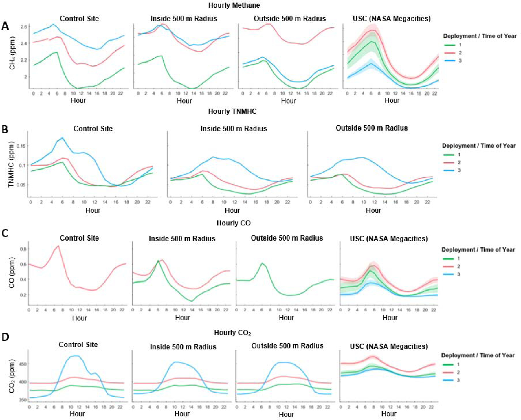
Concentrations grouped by hour of day for (L to R): a control site; pods within the 500 m radius of each facility; pods outside the 500 m radius of each facility; reference data collected by the NASA Megacities project. Each row is a different pollutant: A) Methane; B) TNMHCs; C) CO; D) CO2.

Changes in the height of the planetary boundary layer are primarily driven by convection from the Earth’s surface; as temperatures rise throughout the day, the boundary layer rises (Schindler, 2013). The slightly different elevations of each community are not thought to have significantly impacted these results, as the largest difference in elevation among the three communities was only approximately 50 m (Los Angeles County Public Works, 2020); we expected to see compound concentrations rising and falling at similar times of day for each of the three sites. The inclusion of reference and control site data better informs to what extent seasonality and long-term changes affected our comparison.

Based on the reference data collected by NASA, each of the compounds trended higher during the winter and spring, when the Deployment 2 study took place. This might explain why most concentrations near Deployment 2, the idle site, are higher than near Deployment 1, the first active site. Concentrations appear to be slightly higher during the fall (Deployment 1) than over the summer (Deployment 3), although seasonality did not appear to affect hourly trends or boundary layer differences, only the range of concentrations overall. Since most Y-Pods were placed on one or two story roofs, while the reference instrument inlet was mounted approximately 2 m above the roof of an 11 story commercial building, hourly trends were expected to be slightly staggered due to this significant difference in height. One monitor placed on a seven-story roof throughout the deployment saw trends similar to the Megacities reference data at a similar elevation and building placement as opposed to the rest of the sites, which were closer to ground level. The reference instrument represents the larger seasonal trends over the course of a year, while our monitors show shorter term spatial and temporal differences much closer to human activities.

We also compared the concentrations of TNMHCs against methane in Figure 8; correlation might indicate a shared source. Although there are countless TNMHC sources in the Los Angeles area, narrowing emission events down to when they correlate with methane, which is predominantly associated with oil and gas activities, could identify TNMHCs associated with oil and gas activity. This data was similarly grouped by proximity, control site near the pipeline as well as pods inside and outside the 500 m radius of each site. At Deployment 2, the spreads and linear fits are the most similar to each other while showing the weakest correlations overall. The baseline removed comparisons similarly lack patterns, suggesting that the methane linked to the facility was not accompanied by plumes of other hydrocarbons. At Deployment 1, the trends were the most linear, but once again did not vary significantly based on proximity to oil and gas activity for the full data or baseline removed spikes. The lower overall concentrations throughout this study could explain part of the uniformity. For Deployment 3, while the inside-outside pods have parallel trendlines, we can see several “fingers” diverging from the main plume for the data within the 500 m radius of the oil and gas facility only. This suggests that at certain times, TNMHCs and methane are extremely well correlated and likely associated with oil and gas emissions. The baseline removed data furthers this narrative; episodic spikes nearby the site clearly show a much higher correlation than those farther away, once again suggesting that the Deployment 3 site is a more significant source of both compounds than the other sites.

Figure 8.

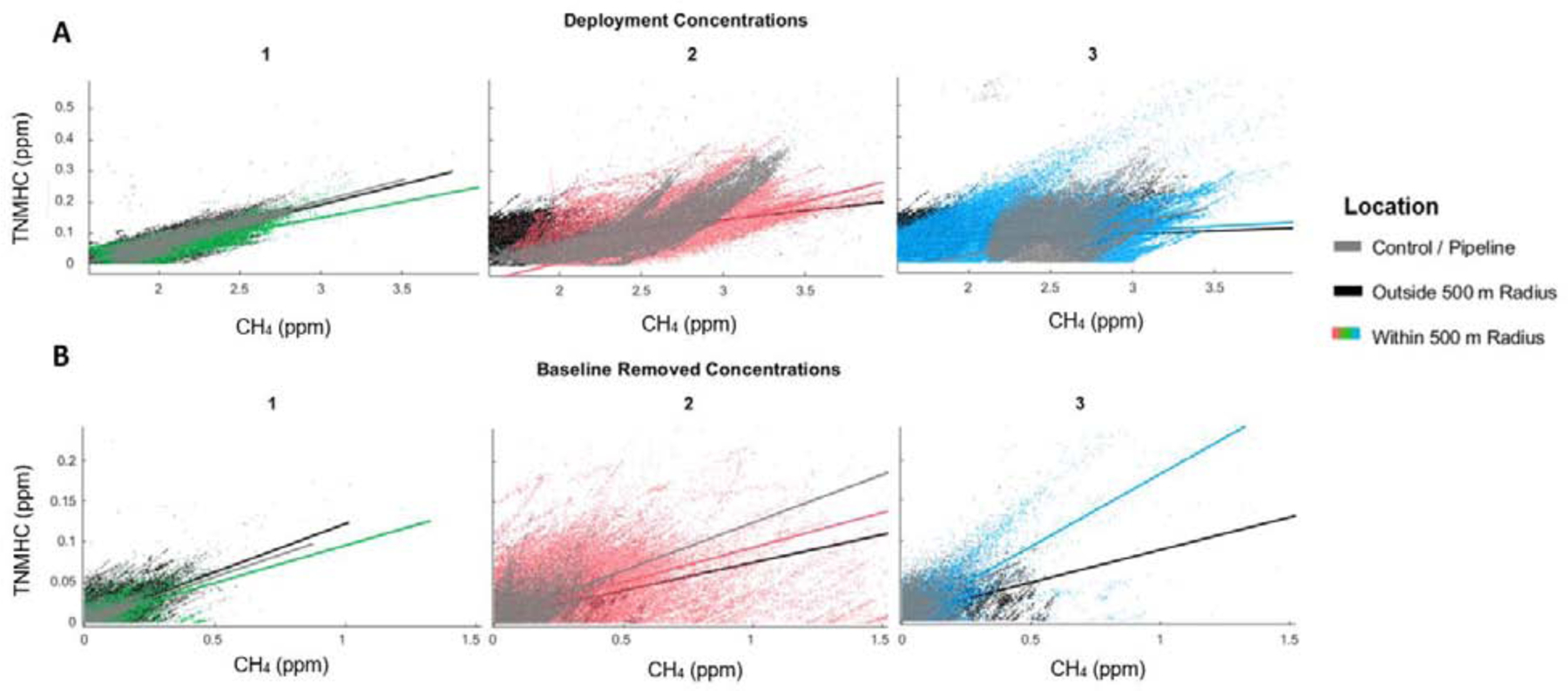
Trends between Methane and TNMHCs colored by location: at the control site, inside the 500 m radius, and outside the radius. The rows are split by: A) deployment data; B) baseline removed data.

As we previously saw, the concentrations of both compounds at the control site varied by study and time of year. Thus, there is not too much uniformity across these plots, although all three show correlations similar or slightly better than those experienced at the other neighborhood locations. The baseline removed plots do not inform much, suggesting that spike events emanating from the pipeline at the control site for both compounds occurred, but not necessarily at the same time.

3.8. CO and CO2 comparison among the three deployments

While CO and CO2 were not extensively studied on their own, since they are the products of combustion activities, they were used as a comparison tool against CH4 and TMHCs to determine what emissions might be associated with combustion events, whether from oil and gas activities or other anthropogenic sources such as auto emissions. Note that CO data was not available from the NASA source for November and December 2016 in Figure 7.

The lack of CO data at the upwind comparison site and throughout the Deployment 3 makes it difficult to draw conclusions about combustion-related emissions in the neighborhood. CO emissions peaked about two hours later at the USC reference site as opposed to our pods; this is likely due to the large differences in height between NASA’s monitors and ours. Peaking around 7am at ground level is consistent with traffic patterns in the early morning. Deployment 2 remains slightly higher than Deployment 1 within the 500 m radius; this same trend was seen at the reference site, signaling that this is likely explained by the time of year, not oil-related activity at the active facility.

For CO2, Deployment 3 saw drastically elevated concentrations all throughout the neighborhood, which may be attributed to plant respiration at ground level during the summer months. It does not appear to be related to episodic flaring or other oil and gas activities due to its widespread recurrence. The neighborhoods studied are considered low-density residential (Liberty Hill Foundation, 2015); many homes in the area have lawns and some have trees, although the area is still urban (Longcore, 2013). While Deployment 1 and Deployment 2 were in agreement both with each other and the seasonal trends shown in the reference data, despite some hourly shifting from the different elevations, these trends are not thought to be necessarily linked to complete combustion or the oil and gas facilities themselves.

3.8. Methane and TNMHCs at the control site during all three deployments

To help assess the seasonal and year-to-year impact on concentration differences, one pod was placed at the same site upwind of the three facilities during each deployment; each time this control site was outside of the 500 m radius and upwind from the oil field. However, we frequently observed relatively elevated concentrations at this control site, as per Figure 7. Upon subsequent investigation, we identified a natural gas distribution pipeline runs along the street where these control pods were sited (SoCal Gas, 2020). Fugitive emissions from the pipeline might explain relatively elevated methane and TNMHC levels at this site and represent another source in the area rather than a true “control” concentration.

In Figure 7, the concentration ranges and hourly trends seen at the control site for each study mirror those seen at the pods nearest oil and gas activities; yearly trends seem to dominate the results we see at each site. The exception to this is the concentrations of methane throughout the Deployment 3 study; concentrations hovered approximately 0.4 ppm higher within the 500 m radius of the facility and at the control site located along the pipeline as opposed to sites in other parts of the community. This signals that the Deployment 3 facility and other oil and gas operations in the area are the main contributors of methane in the neighborhood. The time of year of the Deployment 3 study also saw the lowest concentrations at the USC reference site, furthering the narrative that this elevated methane is from the oil and gas activity in the neighborhood and not influenced by the time of year or other variables in the area. Overall, we expected to see the concentrations of non-reactive compounds such as CH4 rise and fall with the boundary layer itself; each peak roughly around 7am for both our monitors and the reference site accordingly.

The control site was used as the main point of reference for TNMHCs as a reference instrument was not available in the Los Angeles area. Although concentrations for both Deployment 1 and Deployment 2 bottomed out around 2pm each day, TNMHCs all throughout the Deployment 3 neighborhood were elevated and did not level out until between 6 and 8 pm. Two years passed between the first two deployments and the third; shifts in the area over that period could inform why Deployment 3 sees different trends differs from the previous two. The uniformity of emissions across all three locations for all three sites again suggests that the oil and gas operations were not as major a source of TNMHCs as for other compounds, such as methane.

4. Discussion

4.1. Key Findings

This study is one of the first studies on air quality impacts of urban oil drilling, and one of the most comprehensive as it spans four years and three neighborhoods. Chiefly, air quality is a major concern near oil and gas facilities, especially those that have homes, schools, and other sensitive land use within the immediate area. Both methane and TNMHCs are linked to oil and gas activities, with methane being the more significant of the two; the myriad sources of TNMHCs in a complex urban environment are more difficult to disentangle, while methane emissions can be attributed to oil and gas facilities and distribution pipelines with a higher degree of certainty.

Although the daily production and precise activities at each site are murky due to self-reporting and temporal aggregation, we attribute many of the differences among the three sites to be the result of the presence of oil and gas facilities, although some of the larger trends were likely influenced by the year and time of year. Deployment 3 saw the largest spikes of methane and TNMHCs in the immediate vicinity of the facility, while Deployment 2 also recorded large spikes despite being an idle facility. Deployment 1 had the lowest concentrations overall, but this is consistent with the year and time of year trends observed at other reference sites; the spikes surrounding this facility, albeit smaller than those throughout the other two deployments, are consistent with what we consider to be emissions from an active oil and gas facility.

4.2. Environmental Justice Implications

Numerous studies have shown that ambient air pollution is generally worse in low-income and people of color neighborhoods than in their higher income or whiter counterparts (Kim et al., 2019; Dadvand et al., 2015; Lin et al., 2013; Sun et al., 2017). Deploying decentralized neighborhood air quality sensors can facilitate understanding of difference in air quality in diverse and often understudied neighborhoods. Low-income residents are further less likely to be able to mitigate their exposure, as they are less likely to have air conditioning and more likely to leave windows open, increasing their daily exposure to outdoor pollutants (Sun et al., 2017). Several other studies have highlighted how income bracket may dictate a community’s air quality (Lin et al., 2018; Yu et al., 2016; Liu et al., 2016).

Studies have similarly demonstrated that the impacts of drilling, refining, flaring, spills or leaks, and pipelines disproportionately affect people of color and low-income populations across the US (Kroepsch et al., 2019; Johnston et al., 2020). In Los Angeles, California, of the 75 communities the Pacific Pipeline intersects, 74 had higher percentages of people of color, and all 75 had higher percentages of non-English speakers compared to the national average at the time of its construction. In addition, 62 of these neighborhoods had per capita incomes below the national, state, county, and city averages (O’Rourke et al., 2003; Impact Assessment, Inc., 1995). As presented in section 2.2, the specific Los Angeles communities studied in this work are no exception to these trends, with community oil and gas operations affecting communities that are both low income and historically disenfranchised. The inherent inequity of oil and gas infrastructure in Los Angeles is one facet of the environmental justice issues plaguing the city’s Black and Latino members; this study aimed to shed light on the exact pollutant concentrations these Angelenos faced over long periods of time. This exposure data has also been made available to participants in the study, and will be compared with newly-collected health and demographic information in a future work.

4.3. TNMHCs in Urban Communities

In this work, we used TNMHCs as a proxy for VOC sources of potential health concern, generalized into a singular category rather than speciated into individual hydrocarbons. As mentioned in section 1.1, the health risk of TNMHCs depends on the exact compounds emitted, which we were unable to assess in this study. Here, we will reference other TNMHC studies to help put our results in context.

In a six-year study of 28 U.S. cities, the most significant TNMHC source was vehicular emissions, followed by oil and gas activities in cities such as Los Angeles and Baton Rouge (Baker et al., 2007). Another study found that TNMHC concentrations in Cincinnati, Ohio ranged from 0.4 to 3 ppm, while concentrations in Los Angeles hovered between 0.5 and 6 ppm (Altshuller et al., 1966). Concentrations in both cities peaked around heavy traffic times, although the significantly larger range in Los Angeles might be attributed to the different climates, populations, and the prevalence of oil and gas in the latter. Despite this study having taken place in the 1960’s, the three oil and gas facilities analyzed in this study had begun operations around then (California Department of Conservation, 2019). While TNMHC concentrations are bound to be high in most urban areas with heavy traffic, Los Angeles seem to have higher concentrations relative to other cities.

In Los Angeles, SCAQMD studies have found higher concentrations of VOCs at reference sites located nearby or downwind of freeways as opposed to other locations situated further from heavy traffic (SCAMD, 2012). At the reference site utilized in Kern County, CA, typical TNMHC minutely averages ranged from 0 to 1.15 ppm throughout 2019, lower than those noted in our Los Angeles communities. Note that while oil and gas activities are present in this area, the region is considered rural and the site is located approximately 15 km from the nearest freeway. This makes it more difficult to determine if all pods in LA were influenced by traffic activity, or if sensor placement at those nearest freeways was insufficient to pick up on larger trends.

Whether or not these levels are likely to adversely impact human health depends greatly on the exact species of hydrocarbons emitted. While some guidelines are in place in California for non-speciated TNMHCs from specific sources, there are no true limits or guidelines on what concentrations are safe for humans as the level of danger varies significantly based on the specific hydrocarbon (SCAQMD, 2012).

For hydrocarbons that have been linked to cancer, such as benzene, multiple studies by Glass et. al. (2001-2005) suggest that cumulative exposure increases the risk of leukemia at an approximately 2 ppm threshold over the course of a year. However, the same group was unable to pinpoint a threshold for benzene exposure at which there was no risk of adverse health outcomes (Glass et. al., 2001; Glass et. al., 2005). Even at levels below 1 ppm, which is aligned with the episodic spikes in our studies, the risk of other adverse health effects is palpable (Glass et. al., 2003; Smith, 2010). Short-lived spikes may not represent the most worrisome exposure outcomes, but can affect the health of community members nonetheless.

4.4. Limitations & Lessons Learned

For the physical setup of our experiment, since we worked within the constraints of those who were willing to house our monitors, some placements were not ideal. Future recommendations for placement include a mix of upwind and downwind monitors for each deployment and focused on having monitors directly downwind of each oil and gas facility. The studies were also limited by occasional power and data consistency issues. For instance, the one monitor directly downwind of the oil and gas facility during Deployment 1 frequently lost power, rendering the sparse data unusable for our analysis. The loss of data at a key monitoring site hindered our ability to adequately address spatial differences associated with wind direction. Additionally, the monitor location selected as a control site across all three deployments ended up being placed atop a natural gas pipeline, confounding our results as this was an additional, unintended methane source in the area.

Since each of the deployments took place during different years, during different seasons, for different lengths of time, seasonal trends may have affected the comparison among all three sites. Additionally, the production data that the facilities self-report is published monthly, so we cannot examine daily trends with respect to the monitor observations. Based on the results of these studies and the continuing complaints by residents in each area, we have reasons to be skeptical of the self-reported data that has been made available, making it increasingly difficult to draw firm conclusions. These factors confound our ability to assess the cause of elevated concentrations, whether it be seasonal atmospheric conditions, oil and gas activity, another factor, or a combination of these three.

While this is one of the most comprehensive studies to date on urban oil and gas activities in the area, future studies are needed to improve our understanding of impacts as well as mitigation strategies. For instance, conducting each of these studies at the same time of year or even simultaneously would have assured more comparable data. Additionally, since spikes were generally seen downwind of oil and gas facilities, we would recommend placing as many monitors east of the sites as possible to fully understand the aggravated health effects those living or working in those areas may experience in addition to those within the 500 m critical radius. Likewise, the placement of monitors relative to freeways could be improved upon to better understand the influence of traffic on TNMHCs. Access to speciated hydrocarbon data could also be beneficial; colocation with a reference instrument that measures harmful TNMHCs such as benzene could better inform the community of their risk level. Overall, we find that the neighborhood-scale monitoring campaigns provide insights into local sources, episodic emissions events and refined spatial air quality data. This is especially useful in complex urban areas such as Los Angeles, where population density, sources, and the terrain can make air quality events even more localized on small spatial and temporal scales.

4.5. Broader Implications

Although oil and gas activities are not present in most major cities, additional locations face the same unique challenge of having multiple major pollutant sources in a complex urban environment. Other major cities with significant oil and gas activity include Abu Dhabi in the United Arab Emirates, Rio de Janeiro in Brazil, Calgary in Canada, and Houston in the United States (Cunningham, 2015). Over 17 million people in the United States alone live within a mile of an active oil or gas facility (Bienkowski, 2017). Despite the staggering amount of people affected by oil and gas in cities and other areas alike, research on exposure and health effects in proximity to oil and gas remains limited. Few sensor network studies have been utilized in the cities mentioned, and even less attention has been paid to hydrocarbons and oil and gas emissions specifically. Since this study was successful in determining hydrocarbon emissions in a set radius of oil and gas activities, it could be reproducible in other cities, so long as reference-grade instruments are accessible in each location of interest for calibration. Through our field normalization approach, pods need to be co-located in an environment similar to that of the deployment, as the calibration models are not meant to extrapolate. Thus, the availability of reference-grade instruments may be a barrier to replicating this study in other areas of interest, while the use of our sensor network could easily be implemented in another city for source attribution purposes.

5. Conclusions

This is the only multi-year study centering on oil and gas activity in urban Los Angeles, and one of the only focusing on the impacts on homes and schools in the immediate area. It also compares multiple facilities drawing from the same oilfield, taking the production data at each site into account. Over the three years of monitoring deployments, the differences in the concentration ranges among the three are thought to be mostly attributed to differences in yearly and monthly trends rather than the oil and gas facilities themselves. We continued to observe elevated local emissions near the idle well site indicating the potential role that fugitive emissions or maintenance activities can have on local air quality. The presence of oil and gas facilities lead to elevated air pollutant concentrations, specifically methane, in the surrounding neighborhoods.

Highlights:

• Methane emissions were heightened near urban oil and gas facilities

• An oil and gas facility registered as inactive still appears to emit methane

• TNMHC spikes may be related to oil and gas activity

• Natural gas distribution pipelines may also be a source of fugitive methane emissions

• Sensor networks highlight spatial and temporal differences at neighborhood scale

References

- Adgate JL, Goldstein BD, & Mckenzie LM (2014). Potential Public Health Hazards, Exposures and Health Effects from Unconventional Natural Gas Development. Environmental Science & Technology, 48(15), 8307–8320. doi: 10.1021/es404621d [DOI] [PubMed] [Google Scholar]
- Allen DT, Torres VM, Thomas J, Sullivan DW, Harrison M, Hendler A, Seinfeld JH (2013). Measurements of methane emissions at natural gas production sites in the United States. Proceedings of the National Academy of Sciences, 110(44), 17768–17773. doi: 10.1073/pnas.1304880110 [DOI] [PMC free article] [PubMed] [Google Scholar]
- Altshuller AP, Ortman GC, Saltzman BE, Neligan RE (1966). Continuous Monitoring of Methane and Other Hydrocarbons In Urban Atmospheres. Journal of the Air Pollution Control Association, 16:2, 87–91. doi: 10.1080/00022470.1966.10468448 [DOI] [PubMed] [Google Scholar]
- Baker AK, Beyersdorf AJ, Doezema LA, Katzenstein A, Meinardi S,Simpson IJ, Blake D, & Rowland FS (2007). Measurements of nonmethane hydrocarbons in 28 United States cities. Atmospheric Environment, 42 (2008) 170–182. doi: 10.1016/j.atmosenv.2007.09.007. [DOI] [Google Scholar]
- Bienkowski B (2017). 17 million in US live near active oil or gas wells Environmental Health News, ehn.org. [Google Scholar]
- Brienza S, Galli A, Anastasi G, & Bruschi P (2015). A Low-Cost Sensing System for Cooperative Air Quality Monitoring in Urban Areas. Sensors, 15(6), 12242–12259. doi: 10.3390/s150612242 [DOI] [PMC free article] [PubMed] [Google Scholar]
- Brosselin P, Rudant J, Orsi L, Leverger G, Baruchel A, Bertrand Y, Nelken B, Robert A, Michel G, Margueritte G, Perel Y, Mechinaud F, Bordigoni P, Hemon D, & Clavel J (2009). Acute childhood leukaemia and residence next to petrol stations and automotive repair garages: the ESCALE study (SFCE). Occupational and Environmental Medicine, 66(9), 598–606. doi: 10.1136/oem.2008.042432 [DOI] [PubMed] [Google Scholar]
- California Census Bureau. (2020). Data. Census.Ca.Gov https://census.ca.gov/htc-map/
- California Department of Conservation. (2018, April 27). Well Search Retrieved from https://www.conservation.ca.gov/calgem
- California Department of Conservation, Notice to Operators: Voluntary Reporting of Hydraulic Fracture Stimulation Operations, March 28, 2012.
- Casey JG, Collier-Oxandale A, & Hannigan M (2019). Performance of artificial neural networks and linear models to quantify 4 trace gas species in an oil and gas production region with low-cost sensors. Sensors and Actuators B: Chemical, 283, 504–514. doi: 10.1016/j.snb.2018.12.049 [DOI] [Google Scholar]
- Civan F (2015). Reservoir Formation Damage (3rd ed.). Gulf Professional Publishing. doi: 10.1016/C2014-0-01087-8 [DOI] [Google Scholar]
- Clements AL, Griswold WG, Rs A, Johnston JE, Herting MM, Thorson J, . . . Hannigan M (2017). Low-Cost Air Quality Monitoring Tools: From Research to Practice (A Workshop Summary). Sensors, 17(11), 2478. doi: 10.3390/s17112478 [DOI] [PMC free article] [PubMed] [Google Scholar]
- Colburn T, Kwiatkowski C, Schultz K, & Bachran M (2011). Natural Gas Operations from a Public Health Perspective. Human and Ecological Risk Assessment: An International Journal, 17(5), 1039–1056. doi: 10.1080/10807039.2011.605662 [DOI] [Google Scholar]
- Collier-Oxandale A, Casey JG, Piedrahita R, Ortega J, Halliday H, Johnston J, & Hannigan M (2018a). Assessing a low-cost methane sensor quantification system for use in complex rural and urban environments. Atmos. Meas. Tech, 11, 3569–3594. doi: 10.5194/amt-11-3569-2018 [DOI] [PMC free article] [PubMed] [Google Scholar]
- Collier-Oxandale A, Coffey E, Thorson J, Johnston J, & Hannigan M (2018b). Comparing Building and Neighborhood-Scale Variability of CO2 and O3 to Inform Deployment Considerations for Low-Cost Sensor System Use. Sensors, 18(5), 1349. MDPI AG. doi: 10.3390/s18051349 [DOI] [PMC free article] [PubMed] [Google Scholar]
- Collier-Oxandale A, Papapostolou V, Feenstra B, Der Boghossian B, & Polidori A (2020). Lessons Learned from Deploying Low-Cost Air Quality Sensors with 14 California Communities. submitted to Citizen Science Theory and Practice - in review [Google Scholar]
- Collier-Oxandale A, Thorson J, Halliday H, Milford J, & Hannigan M (2019). Understanding the ability of low-cost MOx sensors to quantify ambient VOCs. Atmos. Meas. Tech. Discuss doi: 10.5194/amt-2018-304 [DOI] [Google Scholar]
- Cunningham N (2015). Seven Cities With Economic Fates Tied To The Price Of Crude Oil. EnergyFuse.org. [Google Scholar]
- Cushing LJ, Vavra-Musser K, Chau K, Franklin M, & Johnston JE (2020). Flaring from Unconventional Oil and Gas Development and Birth Outcomes in the Eagle Ford Shale in South Texas. Environmental Health Perspectives, 128, 7. doi: 10.1289/EHP6394 [DOI] [PMC free article] [PubMed] [Google Scholar]
- Dadvand P, Nieuwenhuijsen MJ, Esnaola M, Forns J, Basagaña X, Alvarez-Pedrerol M, . . . Sunyer J (2015). Green spaces and cognitive development in primary schoolchildren. Proceedings of the National Academy of Sciences, 112(26), 7937–7942. doi: 10.1073/pnas.1503402112 [DOI] [PMC free article] [PubMed] [Google Scholar]
- Dahlgren J, Takhar H, Anderson-Mahoney P et al. (2007). Cluster of systemic lupus erythematosus (SLE) associated with an oil field waste site: a cross sectional study. Environ Health 6, 8. doi:/ 10.1186/1476-069X-6-8 [DOI] [PMC free article] [PubMed] [Google Scholar]
- Dey T, Gogoi K, Unni B, Bharadwaz M, Kalita M, Ozah D, et al. (2015) Role of Environmental Pollutants in Liver Physiology: Special References to Peoples Living in the Oil Drilling Sites of Assam. PLoS ONE 10(4): e0123370. doi: 10.1371/journal.pone.0123370 [DOI] [PMC free article] [PubMed] [Google Scholar]
- Eugster W, & Kling GW (2012). Performance of a low-cost methane sensor for ambient concentration measurements in preliminary studies. Atmos. Meas. Tech, 5, 1925–1934. doi: 10.5194/amt-5-1925-2012 [DOI] [Google Scholar]
- Glass D, Gray C, Adams G, Manuell R, Bisby J (2001). Validation of exposure estimation for benzene in the Australian petroleum industry. Toxicol Ind. Health, 17(4):113–27. doi: 10.1191/0748233701th099oa [DOI] [PubMed] [Google Scholar]
- Glass D, Gray C, Jolley D, Gibbons C, Sim M (2005). Health Watch exposure estimates: Do they underestimate benzene exposure? Chem. Biol. Interact, 153–54:23–32. doi: 10.1016/j.cbi.2005.03.006 [DOI] [PubMed] [Google Scholar]
- Glass D, Gray C, Jolley D, Gibbons C, Sim M, Fritschi L, . . . Manuell R (2003). Leukemia Risk Associated with Low-Level Benzene Exposure. Epidemiology, 14(5), 569–577. doi:jstor.org/stable/3703314 [DOI] [PubMed] [Google Scholar]
- Goldstein BD (2010). Benzene as a cause of lymphoproliferative disorders. Chemico-Biological Interactions, 184(1–2), 147–150. doi: 10.1016/j.cbi.2009.12.021 [DOI] [PubMed] [Google Scholar]
- Heimann I, Bright V, Mcleod M, Mead M, Popoola O, Stewart G, & Jones R (2015). Source attribution of air pollution by spatial scale separation using high spatial density networks of low cost air quality sensors. Atmospheric Environment, 113, 10–19. doi: 10.1016/j.atmosenv.2015.04.057 [DOI] [Google Scholar]
- Holloway MD (2018). Fracking: Further Investigations into the Environmental Considerations and Operations of Hydraulic Fracturing (2nd ed.). Beverly, MA: Scrivener Publishing/Wiley. [Google Scholar]
- Hopkins FM, Kort EA, Bush SE, Ehleringer JR, Lai CT, Blake DR, & Randerson JT (2016). Spatial patterns and source attribution of urban methane in the Los Angeles Basin. Journal of Geophysical Research: Atmospheres, 121(5), 2490–2507. doi: 10.1002/2015jd024429 [DOI] [Google Scholar]
- Impact Assess. Inc. (1995). Documentation in Support of Socioeconomic Review Comments to Draft Environmental Impact Statement/Subsequent Environmental Impact Report: Pacific Pipeline Project [Google Scholar]
- Johnson KK, Bergin MH, Russell AG, & Hagler GS (2018). Field Test of Several Low-Cost Particulate Matter Sensors in High and Low Concentration Urban Environments. Aerosol and Air Quality Research, 18(3), 565–578. doi: 10.4209/aaqr.2017.10.0418 [DOI] [PMC free article] [PubMed] [Google Scholar]
- Johnston JE, Chau K, Franklin M, & Cushing L (2020). Environmental Justice Dimensions of Oil and Gas Flaring in South Texas: Disproportionate Exposure among Hispanic communities. American Chemical Society Publications, 54, 10, 6289–6298. doi: 10.1021/acs.est.0c00410 [DOI] [PMC free article] [PubMed] [Google Scholar]
- Johnston JE, Lim E, & Roh H (2019). Impact of upstream oil extraction and environmental public health: A review of the evidence. Science of The Total Environment, 657, 187–199. doi: 10.1016/j.scitotenv.2018.11.483 [DOI] [PMC free article] [PubMed] [Google Scholar]
- Kim J, Shusterman AA, Lieschke KJ, Newman C, & Cohen RC (2017). The BErkeley Atmospheric CO2 Observation Network: Field Calibration and Evaluation of Low-cost Air Quality Sensors. Atmos. Meas. Tech, 11, 1937–1946. doi: 10.5194/amt-2017-339-rc1 [DOI] [Google Scholar]
- Kim S, Senick JA, & Mainelis G (2019). Sensing the invisible: Understanding the perception of indoor air quality among children in low-income families. International Journal of Child-Computer Interaction, 19, 79–88. 10.1016/j.ijcci.2018.12.002 [DOI] [Google Scholar]
- Kirkeleit J, Riise T, Bråtveit M, & Moen BE (2007). Increased risk of acute myelogenous leukemia and multiple myeloma in a historical cohort of upstream petroleum workers exposed to crude oil. Cancer Causes & Control, 19(1), 13–23. doi: 10.1007/s10552-007-9065-x [DOI] [PubMed] [Google Scholar]
- Kudabayeva KI, Bazargaliev YS, Baspakova AM, Darzhanova KB (2014). Estimation of thyroid volume in children from oil-gas producing areas of west Kazakhstan. Biol. Med, 6, 1. [Google Scholar]
- Kroepsch AC, Maniloff PT, Adgate JL, Mckenzie LM, & Dickinson KL (2019). Environmental Justice in Unconventional Oil and Natural Gas Drilling and Production: A Critical Review and Research Agenda. Environmental Science & Technology, 53(12), 6601–6615. doi: 10.1021/acs.est.9b00209 [DOI] [PubMed] [Google Scholar]
- Liberty Hill Foundation. (2015). Drilling Down: The Community Consequences of Expanded Oil Development in Los Angeles [Google Scholar]
- Lin B, & Zhu J (2018). Changes in urban air quality during urbanization in China. Journal of Cleaner Production, 188, 312–321. doi: 10.1016/j.jclepro.2018.03.293 [DOI] [Google Scholar]
- Lin L, Chuang H, Liu I, Chen H, & Chuang K (2013). Reducing indoor air pollution by air conditioning is associated with improvements in cardiovascular health among the general population. Science of The Total Environment, 463–464, 176–181. doi: 10.1016/j.scitotenv.2013.05.093 [DOI] [PubMed] [Google Scholar]
- Liu X, Zhu H, Hu Y, Feng S, Chu Y, Wu Y, Wang C, Zhang Y, Yuan Z, Lu Y (2016). Public’s Health Risk Awareness on Urban Air Pollution in Chinese Megacities: The Cases of Shanghai, Wuhan and Nanchang. Int. J. Environ. Res. Public Health, 13, 845. doi: 10.3390/ijerph13090845 [DOI] [PMC free article] [PubMed] [Google Scholar]
- Longcore T, Li C, & Wilson JP (2004) Applicability of Citygreen Urban Ecosystem Analysis Software to a Densely Built Urban Neighborhood, Urban Geography, 25:2, 173–186, DOI: 10.2747/0272-3638.25.2.173 [DOI] [Google Scholar]
- Los Angeles Almanac (2020). Average Relative Humidity for Los Angeles County, California Retrieved from http://www.laalmanac.com/weather/we19.php
- Los Angeles County Public Works. (2020). LA County Engineer Topography Maps Retrieved from https://pw.lacounty.gov/smpm/cetopo/
- McKenzie L, Blair B, Hughes J, Allshouse WB, Blake N, Helmig D, Milmoe P, Halliday H, Blake D, & Adgate J (2018). Ambient Nonmethane Hydrocarbon Levels Along Colorado’s Northern Front Range: Acute and Chronic Health Risks. Environmental Science & Technology, 52 (8), 4514–4525. doi: 10.1021/acs.est.7b05983 [DOI] [PubMed] [Google Scholar]
- McKenzie LM, Guo R, Witter RZ, Savitz DA, Newman LS, & Adgate JL (2014). Birth Outcomes and Maternal Residential Proximity to Natural Gas Development in Rural Colorado. Environmental Health Perspectives, 122(4), 412–417. doi: 10.1289/ehp.1306722 [DOI] [PMC free article] [PubMed] [Google Scholar]
- Methane: Your Environment, Your Health (2017). National Library of Medicine https://toxtown.nlm.nih.gov/chemicals-and-contaminants/methane
- O’Rourke D, & Connolly S (2003). Just Oil? The Distribution Of Environmental And Social Impacts Of Oil Production And Consumption. Annual Review of Environment and Resources, 28(1), 587–617. doi: 10.1146/annurev.energy.28.050302.105617 [DOI] [Google Scholar]
- Piedrahita R, Xiang Y, Masson N, Ortega J, Collier A, Jiang Y, . . . Shang L (2014). The next generation of low-cost personal air quality sensors for quantitative exposure monitoring. Atmospheric Measurement Techniques, 7(10), 3325–3336. doi: 10.5194/amt-7-3325-2014 [DOI] [Google Scholar]
- Popoola OA, Carruthers D, Lad C, Bright VB, Mead MI, Stettler ME, . . . Jones RL (2018). Use of networks of low cost air quality sensors to quantify air quality in urban settings. Atmospheric Environment, 194, 58–70. doi: 10.1016/j.atmosenv.2018.09.030 [DOI] [Google Scholar]
- Purpleair.com. 2020. Map [online] Available at: https://www.purpleair.com/map?opt=1/mAQI/a10/cC0#1/−10.3/−111.2
- Sadighi K, Coffey E, Polidori A, Feenstra B, Lv Q, Henze D, & Hannigan M (2018). Intra-urban spatial variability of surface ozone in Riverside, CA: viability and validation of low-cost sensors. Atmos. Meas. Tech, 11, 1777–1792. Doi: 10.5194/amt-11-1777-2018 [DOI] [Google Scholar]
- Schindler TL (2013, May 16). Never at rest: The air over Los Angeles Retrieved from https://svs.gsfc.nasa.gov/4077 [Google Scholar]
- Shamasunder B, Collier-Oxandale A, Blickley J, Sadd J, Chan M, Navarro S, Hannigan M, & Wong N (2018). Community-Based Health and Exposure Study around Urban Oil Developments in South Los Angeles. Int. J. Environ. Res. Public Health, 15, 138. doi: 10.3390/ijerph15010138 [DOI] [PMC free article] [PubMed] [Google Scholar]
- Smith MT (2010). Advances in Understanding Benzene Health Effects and Susceptibility. Annu. Rev. Public Health, 2010.31:133–48. doi: 10.1146/annurev.publhealth.012809.103646 [DOI] [PMC free article] [PubMed] [Google Scholar]
- SoCal Gas (2020). Natural Gas Distribution Pipelines in Los Angeles Southern California Gas Company. [Google Scholar]
- South Coast Air Quality Management District. (2012). Ambient Concentrations of Criteria and Air Toxic Pollutants in Close Proximity to a Freeway with Heavy-Duty Diesel Traffic: Final Report Retrieved from: http://www.aqmd.gov/home/air-quality/air-quality-studies/air-quality-monitoring-studies
- South Coast Air Quality Management District. (2012). Ambient Measurements of Air Toxic Pollutants at Resurrection Catholic School in Boyle Heights: Final Report Retrieved from: http://www.aqmd.gov/home/air-quality/air-quality-studies/air-quality-monitoring-studies
- South Coast Air Quality Management District. (2020). About Retrieved from http://www.aqmd.gov/nav/about
- South Los Angeles and Southeast Los Angeles Community Draft EIR. (2016). Retrieved from https://planning.lacity.org/EIR/SouthAndSoutheastLA/DEIR/files/4.11%20Mineral%20Resources.pdf
- Southern California Public Radio. (2016, June 10). Deployment 2 to pay $1.25 million to LA in lawsuit settlement Retrieved from https://www.scpr.org/news/2016/06/09/61494/Deployment2-oil-company-to-pay-1-25-million-to-la-in-l/
- Tran KV, Casey JA, Cushing LJ, & Morello-Frosch R (2020). Residential Proximity to Oil and Gas Development and Birth Outcomes in California: A Retrospective Cohort Study of 2006–2015 Births. Environmental Health Perspectives, 128, 6. doi: 10.1289/EHP5842 [DOI] [PMC free article] [PubMed] [Google Scholar]
- Sun C, Kahn ME, & Zheng S (2017). Self-protection investment exacerbates air pollution exposure inequality in urban China. Ecological Economics, 131, 468–474. doi: 10.1016/j.ecolecon.2016.06.030 [DOI] [Google Scholar]
- Verhulst KR, Karion A, Kim J, Salameh PK, Keeling RF, Newman S, Miller J, Sloop C, Pongetti T, Rao P, Wong C, Hopkins FM, Yadav V, Weiss RF, Duren R, and Miller CE (2017). Carbon Dioxide and Methane Measurements from the Los Angeles Megacity Carbon Project: 1. Calibration, Urban Enhancements, and Uncertainty Estimates, Atmos. Chem. Phys, doi: 10.5194/acp-2016-850, 2017 (in press). [DOI] [PMC free article] [PubMed] [Google Scholar]
- Vikram S, Collier-Oxandale A, Ostertag MH, Menarini M, Chermak C, Dasgupta S, . . . Griswold WG (2019). Evaluating and Improving the Reliability of Gas-Phase SensorSystem Calibrations Across New Locations for AmbientMeasurements and Personal Exposure Monitoring. Atmos. Meas. Tech, 12, 4211. doi: 10.5194/amt-2019-30-ac1 [DOI] [Google Scholar]
- White N, teWaterNaude J, van der Walt A, Ravenscroft G, Roberts W, & Ehrlich R (2009). Meteorologically estimated exposure but not distance predicts asthma symptoms in schoolchildren in the environs of a petrochemical refinery: a cross-sectional study. Environmental Health, 8(1), 45. doi: 10.1186/1476-069x-8-45 [DOI] [PMC free article] [PubMed] [Google Scholar]
- Willis M, Hystad P, Denham E, Hill E (2020). Natural gas development, flaring practices and paediatric asthma hospitalizations in Texas. International Journal of Epidemiology doi: 10.1093/ije/dyaa115 [DOI] [PMC free article] [PubMed] [Google Scholar]
- Yermukhanova L, Zhexenova A, Izimbergenova G, Turebaev M, Bekbauova A, Zumabekov E, et al. (2017). Immunodeficiency states in persons residing in the oil-producing regions of Kazakhstan. Res. J. Med. Sci, 11, 16–18. [Google Scholar]
- Yu H, & Stuart AL (2016). Exposure and inequality for select urban air pollutants in the Tampa Bay area. Science of The Total Environment, 551–552, 474–483. doi: 10.1016/j.scitotenv.2016.01.157 [DOI] [PubMed] [Google Scholar]
Associated Data
This section collects any data citations, data availability statements, or supplementary materials included in this article.