Multi-task multi-modality SVM for early COVID-19 Diagnosis using chest CT data

Abstract

In the early diagnosis of the Coronavirus disease (COVID-19), it is of great importance for either distinguishing severe cases from mild cases or predicting the conversion time that mild cases would possibly convert to severe cases. This study investigates both of them in a unified framework by exploring the problems such as slight appearance difference between mild cases and severe cases, the interpretability, the High Dimension and Low Sample Size (HDLSS) data, and the class imbalance. To this end, the proposed framework includes three steps: (1) feature extraction which first conducts the hierarchical segmentation on the chest Computed Tomography (CT) image data and then extracts multi-modality handcrafted features for each segment, aiming at capturing the slight appearance difference from different perspectives; (2) data augmentation which employs the over-sampling technique to augment the number of samples corresponding to the minority classes, aiming at investigating the class imbalance problem; and (3) joint construction of classification and regression by proposing a novel Multi-task Multi-modality Support Vector Machine (MM-SVM) method to solve the issue of the HDLSS data and achieve the interpretability. Experimental analysis on two synthetic and one real COVID-19 data set demonstrated that our proposed framework outperformed six state-of-the-art methods in terms of binary classification and regression performance.

1. Introduction

Coronavirus disease 2019 (aka COVID-19) has caused more than 170 million confirmed cases and over 3 million confirmed deaths as of June 2021. Recently, a large number of interests have been focused on designing computer-aided diagnosis methods to conduct early COVID-19 diagnosis for reducing the clinician’s workloads and taking care of the confirmed patients early. To this end, medical imaging data such as Real-time reverse Transcription Polymerase Chain Reaction (RT-PCR), chest Computed Tomography (CT) imaging data, and chest X-ray imaging data, have widely been applied to COVID-19 diagnosis such as segmentation (Fan, et al., 2020, Xie et al., 2020) and diagnosis (Kang, et al., 2020, Ouyang, et al., 2020). The machine learning technique is thus becoming one of the effective computer-aided diagnosis methods for the diagnosis and prediction of the COVID-19 disease using medical imaging data.

In the study of early COVID-19 diagnosis, Fang et al. employed Support Vector Machine (SVM) to separate the COVID-19 patients from other pneumonia patients (Fang, et al., 2020). Wang et al. used deep learning methods to first generate deep features from the chest CT images and then conduct the COVID-19 diagnosis using the decision tree and Adaboost (Wang, et al., 2020). In real applications, it is also crucial to predict the development of patient disease by constructing regression models to evaluate the patient’s condition (Zhang, Lai, et al., 2019). For example, Qi et al. employed linear regression and random forest to predict the number of days for COVID-19 patients staying in hospitals (Qi, et al., 2020) and Hamzah et al. proposed to forecast the large-scale outbreak time on the global world (Hamzah, et al., 2020). Chimmula et al. used the Long Short-Term Memory (LSTM) framework to forecast the future confirmed COVID-19 cases in Canada (Chimmula & Zhang, 2020) and Hu et al. proposed a modified stacked autoencoder model to predict the confirmed COVID-19 cases (Hu, Ge, Jin, & Xiong, 2020). Furthermore, the previous study showed that each task may have individual characteristics different from others in multi-task learning (Gan, et al., 2021, Zhang, Liu, et al., 2019), which can thus improve the diagnosis effectiveness with the help of complementary information across all tasks. For example, Bai et al. proposed an LSTM model to identify severe patients as well as predict the patients with potentially malignant progression (Bai, et al., 2020). Zhu et al. integrated the logistic regression with the linear regression to conduct joint classification and regression for early diagnosis of COVID-19 disease (Zhu, et al., 2021).

This paper focuses on designing a new multi-task model to jointly distinguish mild COVID-19 cases from severe cases and predict the conversion time that mild case converts to severe case using the chest CT scans data, by taking into account the importance and the challenges for early diagnosis of COVID-19 disease. Specifically, the confirmed COVID-19 cases can be further categorized into two subgroups, i.e., mild cases and severe cases. If the severe cases can correctly be distinguished from mild cases, mild cases can stay at home while severe cases should be treated at hospitals. As a result, the clinicians’ workloads will be significantly reduced, and severe cases can be treated in time. However, it is challenging to identify mild cases from severe cases and simultaneously predict the conversion time.

Firstly, COVID-19 cases and Healthy Control (HC) are easy to identify since their appearance differences are significant in the chest CT scans based on previous literature (Shi, Wang, et al., 2020, Tang, et al., 2020). However, it is difficult to identify between mild cases and severe cases since their differences in infected lesions are usually small in the chest CT scans, as well as their appearances are similar to other pneumonia with a very slight difference (Guan, et al., 2020). Second, the limited positive subjects are can be used for early diagnosis of COVID-19, but they may lead to some issues, such as the class imbalance and the high dimension and low sample size (HDLSS). For example, the classification models developed for imbalanced data sets often classify the minority class as the majority class to output high false negatives (i.e., low sensitivity) (Zhu, et al., 2021). Moreover, the HDLSS data indicate more features in the data set than the number of subjects, which is often the case in medical imaging data (Hao et al., 2020, Hu, et al., 2021). The HDLSS data make it difficult to construct effective learning models and easily result in the issue of the curse of dimensionality for data analysis (Peng, et al., 2021, Shen et al., 2020, Zhu et al., 2020). Third, it is necessary to conduct a unified framework for both classification and regression/prediction, which not only obtains mutual promotion between different tasks, but it also achieves the interpretability (Zhu, Ma, et al., 2021, Zhu, et al., 2021).

To address aforementioned issues, in this paper, we investigate a new framework for early diagnosis of COVID-19, which jointly distinguish mild COVID-19 cases from severe cases and also predict the conversion time that the mild case will convert to the severe case using the chest CT scans data. To this end, we first segment the whole lung into 26 parts based on both the infection locations and the spreading patterns of the COVID-19 disease to extract three kinds of handcrafted features for each part, aiming at detecting infected lesions and capturing the slight appearance difference between mild cases and severe cases. Then, we employ the Synthetic Minority Over-sampling TEchnique (SMOTE) (Chawla, Bowyer, Hall, & Kegelmeyer, 2002) to generate new samples for the minority class (i.e., severe cases in this work) to solve the issue of the class imbalance. We further propose a new Multi-task Multi-modality Support Vector Machine (MM-SVM) method to extract the common information across multi-modality data as well as multiple tasks to simultaneously capture the slight appearance difference as well as to conduct feature selection, disease diagnosis, and conversion time prediction.

Compared to previous methods, the contributions of the proposed method are listed as follows.

• •Our proposed framework simultaneously solves various issues such as the slight appearance difference between mild cases and severe cases, the interpretability, the HDLSS issue, the class imbalance problem, and the joint classification and regression. Previous methods only focused on a subset of the above issues. For example, Zhu et al. proposed to solve the class imbalance problem, the issue of the HDLSS data, and the joint classification and regression (Zhu, et al., 2021). Besides, Hu et al. conducted a model to solve the interpretability, the class imbalance problem (Hu, et al., 2021). Moreover, Kang, et al. (2020) and Wu, et al. (2020) employed multi-modality data to leave the issues (i.e., the class imbalance problem and the interpretability) alone.
• •This paper proposed a new SVM framework to overcome the issues of early diagnosis of COVID-19. To our knowledge, it is the first work to design the SVM framework to simultaneously conduct multi-task learning and multi-modality learning for medical image analysis. In the literature, Zhang et al. proposed to separately conduct feature selection and disease diagnosis (Zhang, Shen, Alzheimer’s Disease Neuroimaging Initiative, et al., 2012). Moreover, our experimental results show the effectiveness of our proposed framework by outperforming all comparison methods, in terms of binary classification and prediction performance.

In this paper, we denote matrices, vectors, and scalars, respectively, as boldface upper-case letters, boldface lower-case letters, and normal italic letters, as well as denote the Frobenius norm and ${\ell }_{2,1}$-norm of a matrix $\mathbf{M}$, respectively, as ${\Vert \mathbf{M}\Vert }_F=\sqrt{{\sum }_{i,j}{m}_{i,j}^2}$ and ${\Vert \mathbf{M}\Vert }_{2,1}={\sum }_i\sqrt{{\sum }_j{m}_{i,j}^2}$. We further denote the diagonal operator, the transpose operator, the trace operator, and the inverse of the matrix $\mathbf{M}$ as $diag\left(\mathbf{M}\right)$, ${\mathbf{M}}^T$, $tr\left(\mathbf{M}\right)$, and ${\mathbf{M}}^{-1}$.

More specifically, given the multi-modality data $\mathbf{X}=\{{\mathbf{X}}^{\left(1\right)},\dots ,{\mathbf{X}}^{\left(V\right)}\}$ and each modality ${\mathbf{X}}^{\left(v\right)}\in {\mathbb{R}}^{d^{\left(v\right)}\times n}$ where $V$, $d^{\left(v\right)}$, and $n$, respectively, are the number of modalities, the number of features and the number of samples for the v-th modality data, we denote ${\mathbf{x}}_{i,\cdot }^{\left(v\right)}$, ${\mathbf{x}}_{\cdot ,j}^{\left(v\right)}$, and ${\mathbf{x}}_{i,j}^{\left(v\right)}$, respectively, as the $i$th row, the $j$th column, and the element in the $i$th row and the $j$th column. We also denote $\mathbf{y}\in {\{+1,-1\}}^{1\times n}$ and $\mathbf{z}\in {\mathbb{R}}^{1\times n}$ as the ground truth of the classification task and the ground truth of the regression task, respectively.

The proposed framework shown in Fig. 1 involves three steps, i.e., (1) feature extraction which first segments the chest CT scans with hierarchical structures for detecting the slight appearance difference between two classes and then extracts multi-modality handcrafted features for each segment; (2) data augmentation which solves the issue of the class imbalance by augmenting the minority samples; and (3) the MM-SVM method which jointly conducts feature selection, the classification task, and the regression task to achieve the interpretability and solve the issues of the HDLSS data.

Fig. 1.

The flowchart of the proposed framework with three steps: (1) Feature extraction for extracting three set of handcrafted features; (2) Data augmentation for generating the synthetic data for the minority class, i.e., severe COVID-19 cases; (3) The proposed Multi-task Multi-modality SVM (MM-SVM) method for jointly conducting feature selection, classification task, and regression task.

1.1. Feature extraction

It needs to be stated that all the imaging data pre-processing (Shan, et al., 2020, Shi, et al., 2020) and handcrafted feature extraction are processed by experts in pneumonia to guarantee the rationality and reliability of the obtained data for model construction (Song, et al., 2014). Moreover, different from previous deep learning models (Kang, et al., 2020, Wu, et al., 2020) which take the whole image data as the input to output deep representations, the advantages of segmenting an image into multiple semantic regions can be summarized as follows, (1) multiple semantic regions division are obtained by experts in pneumonia to guarantee the rationality and reliability of the obtained data. (2) Each COVID-19 chest CT image is segmented into multiple semantic regions based on the disease characteristics, such as infection locations and spreading patterns. (3) Each handcrafted feature obtained from the multiple semantic regions is guaranteed to be interpretable.

1.2. Data augmentation

The class imbalance problem implies that the distribution of the samples/subjects across all classes is biased or skewed (Chawla et al., 2002, He and Garcia, 2009). Moreover, the sample numbers in different classes can vary from a slight bias to a severe imbalance, e.g., 100 severe cases vs. 322 mild cases in this work. The class imbalance problem poses a challenge for data analysis as most machine learning methods were designed assuming an equal number of subjects for each class (Liu, Wu, & Zhou, 2008). As a consequence, the minority class has poor prediction performance because these methods directly predict the minority class as the labels of the majority class to result in high prediction accuracy but high false-negative (i.e., low sensitivity). However, in real applications, the minority class is more important, compared to the majority class (Galar et al., 2011, Longadge and Dongre, 2013), e.g., distinguishing severe cases from mild cases.

In the literature, the solutions to the class imbalance problem can be categorized into three types, i.e., data pre-processing methods (Zhu et al., 2020), algorithm methods (Zhu, Yang, Zhang, & Zhang, 2019), and sample selection methods (Shen et al., 2020, Yuan et al., 2021). Data pre-processing methods use the resampling techniques to generate synthetic data for the minority classes or reduce the samples of the majority classes, such as the undersampling method, the oversampling method (e.g., Synthetic Minority Oversampling TEchnique (SMOTE)). Algorithm methods focus on designing new machine learning techniques to directly deal with the class imbalance problem, such as cost-sensitive learning, one-class classification, and ensemble methods. Sample selection methods employ the self-paced learning methods or the half-quadratic optimization (Shen et al., 2020) to assign less important samples in the majority classes with small or zero weights.

In this work, considering the issue of the HDLSS data and the class imbalance problem, we employ the oversampling technique (i.e., SMOTE Chawla et al., 2002) to generate synthetic samples for the minority class. More specifically, SMOTE adds the nearest neighbors of each minority sample to augment the samples of the minority classes by the following steps: (1) calculating the $k$ nearest neighbors for each minority sample $\mathbf{x}$. (2) generating a new minority sample ${\mathbf{x}}^{\prime }$ for each minority sample $\mathbf{x}$ by ${\mathbf{x}}^{\prime }=\mathbf{x}+\tau |\mathbf{x}-{\mathbf{x}}_k|$ where $\tau$ is a random number between 0 and 1, and ${\mathbf{x}}_k$ is randomly selected from the nearest neighbors of $\mathbf{x}$. For example, in this work, we generate 100 × 2 synthetic minority samples to have a final balanced data set with 300 minority samples and 322 majority samples for the real COVID-19 dataset.

1.3. Multi-task multi-modality SVM

1.3.1. SVM for classification and regression

SVM was designed to search the maximal margin to conduct the binary classification, aka Support Vector Classification (SVC), by the following objective function (Cortes & Vapnik, 1995).

$$\begin{array}{c}\underset{\mathbf{w},b_w}{min}\frac{1}{2}{\Vert \mathbf{w}\Vert }^2+C_1\sum _{i=1}^n{\xi }_i\hfill \\ s.t.,y_i\left(({\mathbf{x}}_{i,\cdot }^T\mathbf{w}+b_w)\right)\ge 1-{\xi }_i,{\xi }_i\ge 0,i=1,\dots ,n.\hfill \end{array}$$ (1)

where $\mathbf{w}\in {\mathbb{R}}^d$ is the weight vector, $b_w$ is the bias value, $\mathit{\xi }$ is the slack variable, $\mathbf{y}=[y_1,\dots ,y_n]$ is the ground truth of the labels, and $C_1$ is the tuning parameter.

The characteristics (e.g., the sparse solution and the good generalization) make the SVM available for solving the regression problems (Vapnik, 1999), i.e., Support Vector Regression (SVR). Specifically, defining the convex $\epsilon$-insensitive loss function and the slack variables (e.g., $\mathit{\eta }$ and $\hat{\mathit{\eta }}$) to reduce the influence of outliers, the objective function of SVR is formulated as follows:

$$\begin{array}{c}\underset{\mathbf{u},b_u}{min}\frac{1}{2}{\Vert \mathbf{u}\Vert }^2+C_2\sum _{j=1}^{n_1}({\eta }_j,{\hat{\eta }}_j)\hfill \\ s.t.,({\tilde{\mathbf{x}}}_{j,\cdot }^T\mathbf{u}+b_u)-z_j\le \epsilon +{\eta }_j,\hfill \\ z_j-({\tilde{\mathbf{x}}}_{j,\cdot }^T\mathbf{u}+b_u)\le \epsilon +{\hat{\eta }}_j,\hfill \\ {\eta }_j,{\hat{\eta }}_j\ge 0,j=1,\dots ,n_1.\hfill \end{array}$$ (2)

where $\mathbf{u}$ is the weight vector and $b_u$ is the bias value. $\mathbf{z}=[z_1,\dots ,z_{n_1}]$ is the ground truth and $C_2$ is the tuning parameter. In particular, we denote $n$, $n_1$, and $n_2$, respectively, as the number of the whole data set for the classification task (i.e., $n=622$), the original data set for the regression task (i.e., $n_1=422$), and the augmented data set obtained by the SMOTE method in Section 1.2 (i.e., $n_2=200$), i.e., $n=n_1+n_2$. Moreover, we denote ${\tilde{\mathbf{X}}}^{\left(v\right)}\in {\mathbb{R}}^{d^{\left(v\right)}\times n_1}$ and ${\hat{\mathbf{X}}}^{\left(v\right)}\in {\mathbb{R}}^{d^{\left(v\right)}\times n_2}$ ($v=1,\dots ,V$), respectively, as the v-th type feature matrix of the original data set and the augmented data set, i.e., ${\mathbf{X}}^{\left(v\right)}=[{\tilde{\mathbf{X}}}^{\left(v\right)};{\hat{\mathbf{X}}}^{\left(v\right)}]\in {\mathbb{R}}^{d^{\left(v\right)}\times n}$.

1.3.2. Proposed objective function

Given multi-modality data $\mathbf{X}=\{{\mathbf{X}}^{\left(1\right)},\dots ,{\mathbf{X}}^{\left(V\right)}\}$, we integrate Eq. (1) with Eq. (2) to conduct joint classification and regression, i.e., multi-task learning, on the multi-modality data by proposing the objective function as follows:

$$\begin{array}{c}\underset{{\mathbf{w}}^{\left(v\right)},{\mathbf{u}}^{\left(v\right)},b_w,b_u}{min}{C}_1\sum _{i=1}^n{\xi }_i+C_2\sum _{j=1}^{n_1}({\eta }_j,{\hat{\eta }}_j)\hfill \\ +\lambda {\Vert [{\mathbf{w}}^{\left(1\right)},\dots ,{\mathbf{w}}^{\left(V\right)},{\mathbf{u}}^{\left(1\right)},\dots ,{\mathbf{u}}^{\left(V\right)}]\Vert }_{2,1}\hfill \\ s.t.,y_i\left(\sum _{v=1}^V{\alpha }_v({\mathbf{x}}_{i,\cdot }^{{\left(v\right)}^T}{\mathbf{w}}^{\left(v\right)}+b_w)\right)\ge 1-{\xi }_i,\hfill \\ \sum _{v=1}^V{\beta }_v({\tilde{\mathbf{x}}}_{j,\cdot }^{{\left(v\right)}^T}{\mathbf{u}}^{\left(v\right)}+b_u)-z_j\le \epsilon +{\eta }_j,\hfill \\ z_j-\sum _{v=1}^V{\beta }_v({\tilde{\mathbf{x}}}_{j,\cdot }^{{\left(v\right)}^T}{\mathbf{u}}^{\left(v\right)}+b_u)\le \epsilon +{\hat{\eta }}_j,\hfill \\ \sum _{v=1}^V{\alpha }_v=1,\sum _{v=1}^V{\beta }_v=1,{\alpha }_v,{\beta }_v\ge 0,\hfill \\ {\xi }_i,{\eta }_j,{\hat{\eta }}_j\ge 0,i=1,\dots ,n,j=1,\dots ,n_1.\hfill \end{array}$$ (3)

where $\mathit{\alpha }=[{\alpha }_1,\dots ,{\alpha }_v,\dots ,{\alpha }_V]$ and $\mathit{\beta }=[{\beta }_1,\dots ,{\beta }_v,\dots ,{\beta }_V]$, respectively, is the weight vector for the classification task and the regression task. It is noteworthy that we use the original data set to conduct the regression task as the class balance problem only affects the classification task.

Although it is a reasonable approach to integrate suitable divisor weights ${\alpha }_v$ and ${\beta }_v$ with different views for the specific task, it is a time-consuming process and needs abundant prior knowledge. Inspired by the literature (Li et al., 2017, Wang et al., 2019), we propose to adjust the weights automatically according to obtained optimal variables and we have

$$\begin{array}{c}\sum _{v=1}^V{\alpha }_v({\mathbf{x}}_{i,\cdot }^{{\left(v\right)}^T}{\mathbf{w}}^{\left(v\right)}+b_w)=1,\hfill \\ \sum _{v=1}^V{\alpha }_v=1,{\alpha }_v\ge 0,i=1,\dots ,n.\hfill \end{array}$$ (4)

and

$$\begin{array}{c}\sum _{v=1}^V{\beta }_v({\tilde{\mathbf{x}}}_{i,\cdot }^{{\left(v\right)}^T}{\mathbf{u}}^{\left(v\right)}+b_u)=1,\hfill \\ \sum _{v=1}^V{\beta }_v=1,{\beta }_v\ge 0,i=1,\dots ,n_1.\hfill \end{array}$$ (5)

The corresponding solutions of $\mathit{\alpha }$ and $\mathit{\beta }$ are

$$\left\{\begin{array}{cc}{\alpha }_v=\frac{\sum _{i=1}^n({\mathbf{x}}_{i,\cdot }^{{\left(v\right)}^T}{\mathbf{w}}^{\left(v\right)}+b_w)}{\sum _{v=1}^V\sum _{i=1}^n({\mathbf{x}}_{i,\cdot }^{{\left(v\right)}^T}{\mathbf{w}}^{\left(v\right)}+b_w)},\hfill & \text{(a)}\hfill \\ {\beta }_v=\frac{\sum _{j=1}^{n_1}({\tilde{\mathbf{x}}}_{j,\cdot }^{{\left(v\right)}^T}{\mathbf{u}}^{\left(v\right)}+b_u)}{\sum _{v=1}^V\sum _{j=1}^n({\tilde{\mathbf{x}}}_{j,\cdot }^{{\left(v\right)}^T}{\mathbf{u}}^{\left(v\right)}+b_u)},\hfill & \text{(b)}\hfill \end{array}\right)$$ (6)

Obviously, we see that ${\alpha }_v$ and ${\beta }_v$ is dependent on the target variables ${\mathbf{w}}^{\left(v\right)}$, $b_w$, and ${\mathbf{u}}^{\left(v\right)}$, $b_u$, respectively.

The matrix $[{\mathbf{w}}^{\left(1\right)},\dots ,{\mathbf{w}}^{\left(V\right)},{\mathbf{u}}^{\left(1\right)},\dots ,{\mathbf{u}}^{\left(V\right)}]\in {\mathbb{R}}^{d\times 2V}$ (where $d^{\left(1\right)}=\cdots =d^{\left(V\right)}=d$ in the multi-modality learning in this work) conducts feature selection across all tasks as well as across all modalities. This is our first strategy to deal with the apparent difference between mild cases and severe cases. The motivation is that (1) the features are selected by the common information across all modalities (types of features) and all tasks for detecting slight difference and (2) the features selected across modalities and tasks can detect appearance difference more easily than the features selected from single modality or a single task. Moreover, feature selection can remove the redundant features to solve the issue of the HDLSS data and select important features (i.e., the ROIs) to have interpretability.

By observing that (1) each task (i.e., the classification task and the prediction/regression task) focuses on the same subject and (2) every modality is used to explain the same subject, the consistency across all tasks as well as the consistency across all modalities are our second strategy for identifying the slight appearance between two kinds of COVID-19 cases. To this end, we design the regularization terms as follows:

$$\begin{array}{c}\sum _{p,q=1}^V({\Vert {\tilde{\mathbf{X}}}^{{\left(p\right)}^T}[{\mathbf{w}}^{\left(p\right)},{\mathbf{u}}^{\left(p\right)}]-{\tilde{\mathbf{X}}}^{{\left(q\right)}^T}[{\mathbf{w}}^{\left(q\right)},{\mathbf{u}}^{\left(q\right)}]\Vert }_F^2\hfill \\ +{\Vert {\hat{\mathbf{X}}}^{{\left(p\right)}^T}{\mathbf{w}}^{\left(p\right)}-{\hat{\mathbf{X}}}^{{\left(q\right)}^T}{\mathbf{w}}^{\left(q\right)}\Vert }_F^2).\hfill \end{array}$$ (7)

In Eq. (7), the first term indicates the consistency across all modalities and all tasks for the original data set involving both the classification task and the regression task, while the second term represents the consistency across the modalities for the augmented data set involving the classification task only.

Finally, the objective function of our proposed MM-SVM method can be formulated as follows:

$$\begin{array}{c}\underset{{\mathbf{w}}^{\left(v\right)},{\mathbf{u}}^{\left(v\right)},b_w,b_u}{min}{C}_1\sum _{i=1}^n{\xi }_i+C_2\sum _{j=1}^{n_1}({\eta }_j,{\hat{\eta }}_j)\hfill \\ +\lambda {\Vert [{\mathbf{w}}^{\left(1\right)},\dots ,{\mathbf{w}}^{\left(V\right)},{\mathbf{u}}^{\left(1\right)},\dots ,{\mathbf{u}}^{\left(V\right)}]\Vert }_{2,1}\hfill \\ +\rho \sum _{p,q=1}^V({\Vert {\tilde{\mathbf{X}}}^{{\left(p\right)}^T}[{\mathbf{w}}^{\left(p\right)},{\mathbf{u}}^{\left(p\right)}]-{\tilde{\mathbf{X}}}^{{\left(q\right)}^T}[{\mathbf{w}}^{\left(q\right)},{\mathbf{u}}^{\left(q\right)}]\Vert }_F^2\hfill \\ +{\Vert {\hat{\mathbf{X}}}^{{\left(p\right)}^T}{\mathbf{w}}^{\left(p\right)}-{\hat{\mathbf{X}}}^{{\left(q\right)}^T}{\mathbf{w}}^{\left(q\right)}\Vert }_F^2),\hfill \\ s.t.,y_i\left(\sum _{v=1}^V{\alpha }_v({\mathbf{x}}_{i,\cdot }^{{\left(v\right)}^T}{\mathbf{w}}^{\left(v\right)}+b_w)\right)\ge 1-{\xi }_i,\hfill \\ \sum _{v=1}^V{\beta }_v({\tilde{\mathbf{x}}}_{j,\cdot }^{{\left(v\right)}^T}{\mathbf{u}}^{\left(v\right)}+b_u)-z_j\le \epsilon +{\eta }_j,\hfill \\ z_j-\sum _{v=1}^V{\beta }_v({\tilde{\mathbf{x}}}_{j,\cdot }^{{\left(v\right)}^T}{\mathbf{u}}^{\left(v\right)}+b_u)\le \epsilon +{\hat{\eta }}_j,\hfill \\ \sum _{v=1}^V{\alpha }_v=1,\sum _{v=1}^V{\beta }_v=1,{\alpha }_v,{\beta }_v\ge 0,\hfill \\ {\xi }_i,{\eta }_j,{\hat{\eta }}_j\ge 0,i=1,\dots ,n,j=1,\dots ,n_1.\hfill \end{array}$$ (8)

where $C_1$, $C_2$, $\lambda$, and $\rho$ are the non-negative tuning parameters. The first constraint maximizes the distance of the nearest sample points to the hyperplane and uses ${\xi }_i$ to control the proportion of partial non-support vector errors. The second and the third constraint minimizes the distance of the furthest sample points from the hyperplane in terms of upper bound and lower bound, respectively. The constraints in the fourth row restrict the sum of the parameters (i.e., $\mathit{\alpha }$ and $\mathit{\beta }$) over different types of features to be equal to one, and define each parameter (i.e., ${\alpha }_v$ and ${\beta }_v$) to be non-negative value. The constraints in the fifth row define the non-negative variables, including ${\xi }_i$, ${\eta }_j$, ${\hat{\eta }}_j$.

1.3.3. Optimization

Eq. (8) is not convex for all variables (i.e., ${\mathbf{w}}^{\left(v\right)}$, ${\mathbf{u}}^{\left(v\right)}$, $b_w$, $b_u$), but is convex for every variable by fixing other variables. Hence, in this work, we employ the alternating optimization strategy (Bezdek & Hathaway, 2003) to optimize the variables in Eq. (8). We list the pseudo of the proposed optimization in Algorithm 1 and list the details as follows.

(i) Update ${\mathbf{w}}^{\left(v\right)}$, and $b_w$, by fixing ${\mathbf{u}}^{\left(v\right)}$, and $b_u$.

The optimization of ${\mathbf{w}}^{\left(v\right)}$ is dependent on the optimization of ${\mathbf{w}}^{\left(v^{\prime }\right)}$ ($v\ne v^{\prime }$), so we list the optimization of ${\mathbf{w}}^{\left(v\right)}$ as follows. Given the variables (i.e., ${\mathbf{u}}^{\left(v\right)},b_u$), the objective function with respect to the variables (i.e., ${\mathbf{w}}^{\left(v\right)}$, $b_w$) becomes:

$$\begin{array}{c}\underset{{\mathbf{w}}^{\left(v\right)},b_w}{min}{C}_1\sum _{i=1}^n{\xi }_i+\lambda {\Vert [{\mathbf{w}}^{\left(1\right)},\dots ,{\mathbf{w}}^{\left(V\right)},{\mathbf{u}}^{\left(1\right)},\dots ,{\mathbf{u}}^{\left(V\right)}]\Vert }_{2,1}\hfill \\ +\rho \sum _{v,q=1}^V({\Vert {\tilde{\mathbf{X}}}^{{\left(v\right)}^T}[{\mathbf{w}}^{\left(v\right)},{\mathbf{u}}^{\left(v\right)}]-{\tilde{\mathbf{X}}}^{{\left(q\right)}^T}[{\mathbf{w}}^{\left(q\right)},{\mathbf{u}}^{\left(q\right)}]\Vert }_F^2\hfill \\ +{\Vert {\hat{\mathbf{X}}}^{{\left(v\right)}^T}{\mathbf{w}}^{\left(v\right)}-{\hat{\mathbf{X}}}^{{\left(q\right)}^T}{\mathbf{w}}^{\left(q\right)}\Vert }_F^2)\hfill \\ s.t.,y_i\left(\sum _{v=1}^V{\alpha }_v({\mathbf{x}}_{i,\cdot }^{{\left(v\right)}^T}{\mathbf{w}}^{\left(v\right)}+b_w)\right)\ge 1-{\xi }_i,{\xi }_i\ge 0,i=1,\dots ,n.\hfill \end{array}$$ (9)

It is difficult to directly solve the primal problem in Eq. (9), so we solve its dual problem. To this end, we employ the Augmented Lagrange Multipliers (ALM) method (Gill & Robinson, 2012) to obtain the Lagrangian function of Eq. (9) as:

$$\begin{array}{c}\underset{{\mathbf{w}}^{\left(v\right)},b_w,{\xi }_i}{min}\underset{\mathit{\gamma },\mathit{\delta }}{max}{C}_1\sum _{i=1}^n{\xi }_i-\sum _{i=1}^n{\delta }_i{\xi }_i\hfill \\ +\lambda {\Vert [{\mathbf{w}}^{\left(1\right)},\dots ,{\mathbf{w}}^{\left(V\right)},{\mathbf{u}}^{\left(1\right)},\dots ,{\mathbf{u}}^{\left(V\right)}]\Vert }_{2,1}\hfill \\ +\rho \sum _{v,q=1}^V({\Vert {\tilde{\mathbf{X}}}^{{\left(v\right)}^T}[{\mathbf{w}}^{\left(v\right)},{\mathbf{u}}^{\left(v\right)}]-{\tilde{\mathbf{X}}}^{{\left(q\right)}^T}[{\mathbf{w}}^{\left(q\right)},{\mathbf{u}}^{\left(q\right)}]\Vert }_F^2\hfill \\ +{\Vert {\hat{\mathbf{X}}}^{{\left(v\right)}^T}{\mathbf{w}}^{\left(v\right)}-{\hat{\mathbf{X}}}^{{\left(q\right)}^T}{\mathbf{w}}^{\left(q\right)}\Vert }_F^2)\hfill \\ -\sum _{i=1}^n{\gamma }_i[y_i\left(\sum _{v=1}^V{\alpha }_v({\mathbf{x}}_{i,\cdot }^{{\left(v\right)}^T}{\mathbf{w}}^{\left(v\right)}+b_w)\right)-1+{\xi }_i]\hfill \end{array}$$ (10)

where $\mathit{\delta }$ and $\mathit{\gamma }$ are the Lagrange multipliers.

After the mathematical computation, we obtain:

$$\begin{array}{c}\underset{{\mathbf{w}}^{\left(v\right)},b_w,{\xi }_i}{min}\underset{\mathit{\gamma },\mathit{\delta }}{max}{C}_1\sum _{i=1}^n{\xi }_i-\sum _{i=1}^n{\delta }_i{\xi }_i+\lambda tr\left({\mathbf{w}}^{{\left(v\right)}^T}\mathbf{M}{\mathbf{w}}^{\left(v\right)}\right)\hfill \\ +\rho tr\left({\mathbf{w}}^{{\left(v\right)}^T}\sum _{q=1}^V({\tilde{\mathbf{X}}}^{\left(q\right)}{\tilde{\mathbf{X}}}^{{\left(q\right)}^T}+{\hat{\mathbf{X}}}^{\left(q\right)}{\hat{\mathbf{X}}}^{{\left(q\right)}^T}){\mathbf{w}}^{\left(v\right)}\right)\hfill \\ -\sum _{i=1}^n{\gamma }_i[y_i\left(\sum _{v=1}^V{\alpha }_v({\mathbf{x}}_{i,\cdot }^{{\left(v\right)}^T}{\mathbf{w}}^{\left(v\right)}+b_w)\right)-1+{\xi }_i]\hfill \end{array}$$ (11)

where the matrix $\mathbf{M}$ is the diagonal matrix and each element is defined as $m_{i,i}=\frac{1}{2{\Vert {({\mathbf{w}}^{\left(1\right)},\dots ,{\mathbf{w}}^{\left(V\right)},{\mathbf{u}}^{\left(1\right)},\dots ,{\mathbf{u}}^{\left(V\right)})}_{i,\cdot }\Vert }_2}$, $i=1,\dots ,d^{\left(v\right)}$. However, the optimization of $\mathbf{M}$ is dependent on the value of ${\mathbf{w}}^{\left(v\right)}$ that is unknown. Therefore, we iteratively optimize ${\mathbf{w}}^{\left(v\right)}$ and $\mathbf{M}$. As a result, denoting ${\overline{\mathbf{X}}}^{\left(v\right)}={\mathbf{M}}^{-\frac{1}{2}}{\sum }_{q=1}^V({\tilde{\mathbf{X}}}^{\left(q\right)}+{\hat{\mathbf{X}}}^{\left(q\right)})$ and ${\overline{\mathbf{w}}}^{\left(v\right)}={\mathbf{M}}^{\frac{1}{2}}{\mathbf{w}}^{\left(v\right)}$, we have:

$$\begin{array}{c}\underset{{\overline{\mathbf{w}}}^{\left(v\right)},b_w,{\xi }_i}{min}\underset{\mathit{\gamma },\mathit{\delta }}{max}{C}_1\sum _{i=1}^n{\xi }_i-\sum _{i=1}^n{\delta }_i{\xi }_i\hfill \\ +\lambda tr\left({\overline{\mathbf{w}}}^{{\left(v\right)}^T}{\overline{\mathbf{w}}}^{\left(v\right)}\right)+\rho tr\left({\overline{\mathbf{w}}}^{{\left(v\right)}^T}{\overline{\mathbf{X}}}^{\left(v\right)}{\overline{\mathbf{X}}}^{{\left(v\right)}^T}{\overline{\mathbf{w}}}^{\left(v\right)}\right)\hfill \\ -\sum _{i=1}^n{\gamma }_i[y_i\left(\sum _{v=1}^V{\alpha }_v({\overline{\mathbf{x}}}_{i,\cdot }^{{\left(v\right)}^T}{\overline{\mathbf{w}}}^{\left(v\right)}+b_w)\right)-1+{\xi }_i]\hfill \end{array}$$ (12)

Taking the derivative of Eq. (12) with respect to ${\overline{\mathbf{w}}}^{\left(v\right)}$, $b_w$, and ${\xi }_i$, and then letting the results as zeros, we have:

$$\left\{\begin{array}{cc}{\overline{\mathbf{w}}}^{\left(v\right)}={\left({\mathbf{G}}^{\left(v\right)}\right)}^{-1}\left(\sum _{i=1}^n{\gamma }_i{y}_i\sum _{v=1}^V{\alpha }_v{\overline{\mathbf{x}}}_{i,\cdot }^{\left(v\right)}\right),\hfill & \text{(a)}\hfill \\ \sum _{i=1}^n{\gamma }_i{y}_i=0,\hfill & \text{(b)}\hfill \\ C_1={\gamma }_i+{\delta }_i.\hfill & \text{(c)}\hfill \end{array}\right)$$ (13)

where ${\mathbf{G}}^{\left(v\right)}=\rho {\overline{\mathbf{X}}}^{\left(v\right)}{\overline{\mathbf{X}}}^{{\left(v\right)}^T}+\lambda {\mathbf{I}}_d$ and ${\mathbf{I}}_d$ is an identity matrix. Combining Eq. 1.3.3 with Eq. (12), we have,

$$\begin{array}{c}\underset{\mathit{\gamma }}{max}\sum _{i=1}^n{\gamma }_i-\sum _{i=1}^n\sum _{j=1}^n{\gamma }_i{\gamma }_j{y}_i{y}_j\sum _{v=1}^V{\alpha }_v^2{\overline{\mathbf{x}}}_{i,\cdot }^{{\left(v\right)}^T}{\mathbf{O}}^{\left(v\right)}{\overline{\mathbf{x}}}_{i,\cdot }^{\left(v\right)}\hfill \\ s.t.,\sum _{i=1}^n{\gamma }_i{y}_i=0,0\le {\gamma }_i\le C_1,i=1,\dots ,n.\hfill \end{array}$$ (14)

where ${\mathbf{O}}^{\left(v\right)}={\mathbf{G}}^{{\left(v\right)}^{-1}}-\frac{{\lambda }_v}{2}{\left({\mathbf{G}}^{{\left(v\right)}^{-1}}\right)}^T{\overline{\mathbf{X}}}^{\left(v\right)}{\overline{\mathbf{X}}}^{{\left(v\right)}^T}{\mathbf{G}}^{{\left(v\right)}^{-1}}-\frac{1}{2}{\left({\mathbf{G}}^{{\left(v\right)}^{-1}}\right)}^T{\mathbf{G}}^{{\left(v\right)}^{-1}}$.

We convert Eq. (14) to its minimal optimization problem as:

$$\begin{array}{c}\underset{\mathit{\gamma }}{min}\sum _{i=1}^n\sum _{j=1}^n{\gamma }_i{\gamma }_j{y}_i{y}_j\sum _{v=1}^V{\alpha }_v^2{\overline{\mathbf{x}}}_{i,\cdot }^{{\left(v\right)}^T}{\mathbf{O}}^{\left(v\right)}{\overline{\mathbf{x}}}_{i,\cdot }^{\left(v\right)}-\sum _{i=1}^n{\gamma }_i\hfill \\ s.t.,\sum _{i=1}^n{\gamma }_i{y}_i=0,0\le {\gamma }_i\le C_1,i=1,\dots ,n.\hfill \end{array}$$ (15)

We first decompose the symmetric positive semi-definite (PSD) matrix ${\mathbf{O}}^{\left(v\right)}$ to obtain the equation, i.e., ${\mathbf{O}}^{\left(v\right)}={\mathbf{o}}^{{\left(v\right)}^T}{\mathbf{o}}^{\left(v\right)}$, and then convert the Eq. (15) to

$$\begin{array}{c}\underset{\mathit{\gamma }}{min}\sum _{i=1}^n\sum _{j=1}^n{\gamma }_i{\gamma }_j{y}_i{y}_j{\underset{\_}{\mathbf{x}}}_{i,\cdot }^T{\underset{\_}{\mathbf{x}}}_{i,\cdot }-\sum _{i=1}^n{\gamma }_i\hfill \\ s.t.,\sum _{i=1}^n{\gamma }_i{y}_i=0,0\le {\gamma }_i\le C_1,i=1,\dots ,n.\hfill \end{array}$$ (16)

where ${\underset{\_}{\mathbf{x}}}_{i,\cdot }={\sum }_{v=1}^V{\alpha }_v{\mathbf{o}}^{\left(v\right)}{\overline{\mathbf{x}}}_{i,\cdot }^{\left(v\right)}$. Finally, we employ the SVM solvers (Bottou & Lin, 2007) to obtain the optimal solutions of ${\overline{\mathbf{w}}}^{\left(v\right)}$ and $b_w$ as:

$$\left\{\begin{array}{cc}{\overline{\mathbf{w}}}^{\left(v\right)}={\mathbf{G}}^{{\left(v\right)}^{-1}}\sum _{i\in SV}^n{\gamma }_i{y}_i\sum _{v=1}^V{\alpha }_v{\mathbf{o}}^{\left(v\right)}{\overline{\mathbf{x}}}_{i,\cdot }^{\left(v\right)},\hfill & \text{(a)}\hfill \\ b_w=\frac{1}{\left|SV\right|}\sum _{i\in SV}^n(y_i-\sum _{v=1}^V{\alpha }_v{\overline{\mathbf{x}}}_{i,\cdot }^{{\left(v\right)}^T}{\overline{\mathbf{w}}}^{\left(v\right)}).\hfill & \text{(b)}\hfill \end{array}\right)$$ (17)

where $\left|SV\right|$ denotes the cardinality of the support vector set.

(ii) Update ${\mathbf{u}}^{\left(v\right)}$, and $b_u$, by fixing ${\mathbf{w}}^{\left(v\right)}$, and $b_w$.

The optimization of ${\mathbf{u}}^{\left(v\right)}$ is dependent on the optimization of ${\mathbf{u}}^{\left(v^{\prime }\right)}$ ($v\ne v^{\prime }$), so we list the details of the optimization of ${\mathbf{u}}^{\left(v\right)}$ as follows.

After fixing ${\mathbf{w}}^{\left(v\right)}$, $b_w$, the objective function with respect to the variables (i.e., ${\mathbf{u}}^{\left(v\right)}$, $b_u$) is:

$$\begin{array}{c}\underset{{\mathbf{u}}^{\left(v\right)},b_u}{min}{C}_2\sum _{i=1}^{n_1}({\eta }_i,{\hat{\eta }}_i)+\lambda {\Vert [{\mathbf{w}}^{\left(1\right)},\dots ,{\mathbf{w}}^{\left(V\right)},{\mathbf{u}}^{\left(1\right)},\dots ,{\mathbf{u}}^{\left(V\right)}]\Vert }_{2,1}\hfill \\ +\rho \sum _{q=1}^V{\Vert {\tilde{\mathbf{X}}}^{{\left(v\right)}^T}[{\mathbf{w}}^{\left(v\right)},{\mathbf{u}}^{\left(v\right)}]-{\tilde{\mathbf{X}}}^{{\left(q\right)}^T}[{\mathbf{w}}^{\left(q\right)},{\mathbf{u}}^{\left(q\right)}]\Vert }_F^2\hfill \\ s.t.,\sum _{v=1}^V{\beta }_v({\tilde{\mathbf{x}}}_{i,\cdot }^{{\left(v\right)}^T}{\mathbf{u}}^{\left(v\right)}+b_u)-z_i\le \epsilon +{\eta }_i,\hfill \\ z_i-\sum _{v=1}^V{\beta }_v({\tilde{\mathbf{x}}}_{i,\cdot }^{{\left(v\right)}^T}{\mathbf{u}}^{\left(v\right)}+b_u)\le \epsilon +{\hat{\eta }}_i,{\eta }_i,{\hat{\eta }}_i\ge 0,i=1,\dots ,n_1.\hfill \end{array}$$ (18)

To solve the dual problem of Eq. (18), we first obtain the corresponding Lagrangian function as:

$$\begin{array}{c}\underset{{\mathbf{u}}^{\left(v\right)},b_u,{\eta }_j,{\hat{\eta }}_j}{min}\underset{\mathit{\mu },\hat{\mathit{\mu }},\mathit{\varphi },\hat{\mathit{\varphi }}}{max}{C}_2\sum _{i=1}^{n_1}({\eta }_i,{\hat{\eta }}_i)+\lambda tr\left({\overline{\mathbf{u}}}^{{\left(v\right)}^T}{\overline{\mathbf{u}}}^{\left(v\right)}\right)\hfill \\ +\rho tr\left({\overline{\mathbf{u}}}^{{\left(v\right)}^T}{\mathbf{F}}^{\left(v\right)}{\mathbf{F}}^{{\left(v\right)}^T}{\overline{\mathbf{u}}}^{\left(v\right)}\right)-\sum _{i=1}^{n_1}{\varphi }_i{\eta }_i-\sum _{i=1}^{n_1}{\hat{\varphi }}_i{\hat{\eta }}_i\hfill \\ -\sum _{i=1}^{n_1}{\mu }_i[\epsilon +{\eta }_i-\sum _{v=1}^V{\beta }_v({\overline{\mathbf{x}}}_{i,\cdot }^{{\left(v\right)}^T}{\mathbf{u}}^{\left(v\right)}+b_u)+z_i]\hfill \\ -\sum _{i=1}^{n_1}{\hat{\mu }}_i[\epsilon +{\hat{\eta }}_i-z_i+\sum _{v=1}^V{\beta }_v({\overline{\mathbf{x}}}_{i,\cdot }^{{\left(v\right)}^T}{\mathbf{u}}^{\left(v\right)}+b_u)]\hfill \end{array}$$ (19)

where ${\mathbf{F}}^{\left(v\right)}={\mathbf{M}}^{-\frac{1}{2}}{\sum }_{q=1}^V{\tilde{\mathbf{X}}}^{\left(q\right)}$ and ${\overline{\mathbf{u}}}^{\left(v\right)}={\mathbf{M}}^{\frac{1}{2}}{\mathbf{u}}^{\left(v\right)}$. We then calculate the derivative of the Eq. (19) with respect to the variables ${\overline{\mathbf{u}}}^{\left(v\right)}$, $b_u$, ${\eta }_j$, and ${\hat{\eta }}_j$, and then set their results to zeros to have:

$$\left\{\begin{array}{cc}{\overline{\mathbf{u}}}^{\left(v\right)}={\overline{\mathbf{G}}}^{{\left(v\right)}^{-1}}\sum _{i=1}^{n_1}({\mu }_i-{\hat{\mu }}_i)\sum _{v=1}^V{\beta }_v{\mathbf{f}}_{i,\cdot }^{\left(v\right)},\hfill & \text{(a)}\hfill \\ \sum _{i=1}^{n_1}({\mu }_i-{\hat{\mu }}_i)=0,\hfill & \text{(b)}\hfill \\ C_2={\mu }_i+{\varphi }_i,\hfill & \text{(c)}\hfill \\ C_2={\hat{\mu }}_i+{\hat{\varphi }}_i.\hfill & \text{(d)}\hfill \end{array}\right)$$ (20)

By combining Eq. (20) with Eq. (19), we have

$$\begin{array}{c}\underset{\mathit{\mu },\hat{\mathit{\mu }}}{max}\sum _{i=1}^{n_1}({\mu }_i-{\hat{\mu }}_i)z_i-\sum _{i=1}^{n_1}({\mu }_i+{\hat{\mu }}_i)\epsilon -\sum _{i,j=1}^{n_1}({\mu }_i-{\hat{\mu }}_i)({\mu }_j-{\hat{\mu }}_j){\tilde{\mathbf{f}}}_{i,\cdot }^T{\tilde{\mathbf{f}}}_{i,\cdot }\hfill \\ s.t.,\sum _{i=1}^{n_1}({\mu }_i-{\hat{\mu }}_i)=0,0\le {\mu }_i,{\hat{\mu }}_i\le C_2,i=1,\dots ,n_1.\hfill \end{array}$$ (21)

where ${\tilde{\mathbf{f}}}_{i,\cdot }={\sum }_{v=1}^V{\beta }_v{\overline{\mathbf{o}}}^{\left(v\right)}{\mathbf{f}}_{i,\cdot }^{\left(v\right)}$. We decompose the symmetric positive semi-definite (PSD) matrix ${\overline{\mathbf{O}}}^{\left(v\right)}$ to obtain the equation, i.e., ${\overline{\mathbf{O}}}^{\left(v\right)}={\overline{\mathbf{o}}}^{{\left(v\right)}^T}{\overline{\mathbf{o}}}^{\left(v\right)}$, where ${\overline{\mathbf{O}}}^{\left(v\right)}={\overline{\mathbf{G}}}^{{\left(v\right)}^{-1}}-\frac{{\lambda }_v}{2}{\left({\overline{\mathbf{G}}}^{{\left(v\right)}^{-1}}\right)}^T{\mathbf{F}}^{\left(v\right)}{\mathbf{F}}^{{\left(v\right)}^T}{\overline{\mathbf{G}}}^{{\left(v\right)}^{-1}}-\frac{1}{2}{\left({\overline{\mathbf{G}}}^{{\left(v\right)}^{-1}}\right)}^T{\overline{\mathbf{G}}}^{{\left(v\right)}^{-1}}$ and ${\overline{\mathbf{G}}}^{\left(v\right)}=\rho {\mathbf{F}}^{\left(v\right)}{\mathbf{F}}^{{\left(v\right)}^T}+\lambda {\mathbf{I}}_d$.

Finally, we employ traditional SVM solvers (Bottou & Lin, 2007) to obtain the optimal solutions of ${\overline{\mathbf{u}}}^{\left(v\right)}$ and $b_u$ as:

$$\left\{\begin{array}{cc}{\overline{\mathbf{u}}}^{\left(v\right)}={\overline{\mathbf{G}}}^{{\left(v\right)}^{-1}}\sum _{i\in SV}^{n_1}({\mu }_i-{\hat{\mu }}_i)\sum _{v=1}^V{\beta }_v{\mathbf{o}}^{\left(v\right)}{\mathbf{f}}_{i,\cdot }^{\left(v\right)},\hfill & \text{(a)}\hfill \\ b_u=\frac{1}{\left|SV\right|}\sum _{i\in SV}^{n_1}(z_i+\epsilon -\sum _{v=1}^V{\beta }_v{\mathbf{f}}_{i,\cdot }^{{\left(v\right)}^T}{\overline{\mathbf{u}}}^{\left(v\right)}).\hfill & \text{(b)}\hfill \end{array}\right)$$ (22)

Based on Eqs. (17) and (22), we use the following equations to predict the new test sample ${\mathbf{x}}_{te}=\{{\mathbf{x}}_{te}^{\left(1\right)},\dots ,{\mathbf{x}}_{te}^{\left(V\right)}\}$:

$$\left\{\begin{array}{cc}{y}_{te}=max\{\sum _v^V{\alpha }_v{\mathbf{x}}_{te}^{{\left(v\right)}^T}{\mathbf{w}}^{\left(v\right)}+b_w,0\},\hfill & \text{(a)}\hfill \\ z_{te}=\sum _v^V{\beta }_v{\mathbf{x}}_{te}^{{\left(v\right)}^T}{\mathbf{u}}^{\left(v\right)}+b_u.\hfill & \text{(b)}\hfill \end{array}\right)$$ (23)

1.3.4. Convergence analysis

We prove the convergence of Algorithm 1 to optimize our proposed objective function in Eq. (8) by the following Theorem 1.

Theorem 1

The objective function value of Eq. (8) monotonically decreases until Algorithm 1 converges.

Proof

We first denote $J({\mathbf{w}}^{\left(v\right)},{\mathbf{u}}^{\left(v\right)},b_w,b_u)$ as the objective function value of Eq. (8), and also denote ${{\mathbf{w}}^{\left(v\right)}}^{(t+1)}$, ${{\mathbf{u}}^{\left(v\right)}}^{(t+1)}$, $b_w^{(t+1)}$, and $b_u^{(t+1)}$, as the updated values of ${{\mathbf{w}}^{\left(v\right)}}^{\left(t\right)}$, ${{\mathbf{u}}^{\left(v\right)}}^{\left(t\right)}$, $b_w^{\left(t\right)}$, and $b_u^{\left(t\right)}$, respectively, where $t$ indicates the $t$th iteration.

According to dual coordinate descent method in the literature (Hsieh, Chang, Lin, Keerthi, & Sundararajan, 2008), we find that $\mathit{\gamma }$ in Eq. (16) obtains a global optimal solution. Therefore, we employ the SVM solvers (Bottou & Lin, 2007) which consider Karush–Kuhn–Tucker (KKT) conditions (Boyd, Vandenberghe, & Faybusovich, 2006) to optimize ${\mathbf{w}}^{\left(v\right)}$ and $b_w$ and obtain the optimal solutions.

Based on Eq. , the variable $b_w$ has a closed-form solution, so we have:

$$\begin{array}{c}J({{\mathbf{w}}^{\left(v\right)}}^{(t+1)},{{\mathbf{u}}^{\left(v\right)}}^{(t+1)},b_w^{(t+1)},b_u^{(t+1)})\hfill \\ \le J({{\mathbf{w}}^{\left(v\right)}}^{(t+1)},{{\mathbf{u}}^{\left(v\right)}}^{(t+1)},b_w^{\left(t\right)},b_u^{(t+1)})\hfill \end{array}$$ (24)

Since the optimization of ${\mathbf{w}}^{\left(v\right)}$ is independent on the optimization of ${\mathbf{w}}^{\left(v^{\prime }\right)}$ ($v\ne v^{\prime }$), we first focus on the convergence analysis for the individual modality. Considering that the optimization of ${\mathbf{w}}^{\left(v\right)}$ is in dependent on the optimization $\mathbf{M}$, we obtain:

$$\begin{array}{c}J({\mathbf{w}}^{\left(v\right)},{\mathbf{u}}^{\left(v\right)},b_w,b_u)\hfill \\ =J\left({\mathbf{w}}^{\left(v\right)}\right)+\lambda tr\left({\mathbf{w}}^{{\left(v\right)}^T}\mathbf{M}{\mathbf{w}}^{\left(v\right)}\right)\hfill \end{array}$$ (25)

Based on Eqs. (17), (25), we have:

$$\begin{array}{c}J\left({\mathbf{w}}^{{\left(v\right)}^{(t+1)}}\right)+\lambda \sum _i^{d^{\left(v\right)}}\frac{{\Vert {\left({\mathbf{w}}^{{\left(v\right)}^{(t+1)}}\right)}_{i,\cdot }\Vert }_2^2}{2{\Vert {\left({\mathbf{w}}^{{\left(v\right)}^{\left(t\right)}}\right)}_{i,\cdot }\Vert }_2}\hfill \\ \le J\left({\mathbf{w}}^{{\left(v\right)}^{\left(t\right)}}\right)+\lambda \sum _i^{d^{\left(v\right)}}\frac{{\Vert {\left({\mathbf{w}}^{{\left(v\right)}^{\left(t\right)}}\right)}_{i,\cdot }\Vert }_2^2}{2{\Vert {\left({\mathbf{w}}^{{\left(v\right)}^{\left(t\right)}}\right)}_{i,\cdot }\Vert }_2}\hfill \end{array}$$ (26)

Since ${({\Vert {\left({\mathbf{w}}^{{\left(v\right)}^{(t+1)}}\right)}_{i,\cdot }\Vert }_2-{\Vert {\left({\mathbf{w}}^{{\left(v\right)}^{\left(t\right)}}\right)}_{i,\cdot }\Vert }_2)}^2\ge 0$, we obtain:

$$\begin{array}{c}{\Vert {\left({\mathbf{w}}^{{\left(v\right)}^{(t+1)}}\right)}_{i,\cdot }\Vert }_2-\frac{{\Vert {\left({\mathbf{w}}^{{\left(v\right)}^{(t+1)}}\right)}_{i,\cdot }\Vert }_2^2}{2{\Vert {\left({\mathbf{w}}^{{\left(v\right)}^{\left(t\right)}}\right)}_{i,\cdot }\Vert }_2}\hfill \\ \le {\Vert {\left({\mathbf{w}}^{{\left(v\right)}^{\left(t\right)}}\right)}_{i,\cdot }\Vert }_2-\frac{{\Vert {\left({\mathbf{w}}^{{\left(v\right)}^{\left(t\right)}}\right)}_{i,\cdot }\Vert }_2^2}{2{\Vert {\left({\mathbf{w}}^{{\left(v\right)}^{\left(t\right)}}\right)}_{i,\cdot }\Vert }_2}\hfill \end{array}$$ (27)

By embedding Eq. (27) into Eq. (26), we get:

$$\begin{array}{c}J\left({\mathbf{w}}^{{\left(v\right)}^{(t+1)}}\right)+\lambda \sum _i^{d^{\left(v\right)}}{\Vert {\left({\mathbf{w}}^{{\left(v\right)}^{(t+1)}}\right)}_{i,\cdot }\Vert }_2\hfill \\ \le J\left({\mathbf{w}}^{{\left(v\right)}^{(t+1)}}\right)+\lambda \sum _i^{d^{\left(v\right)}}{\Vert {\left({\mathbf{w}}^{{\left(v\right)}^{\left(t\right)}}\right)}_{i,\cdot }\Vert }_2\hfill \end{array}$$ (28)

After combining with all ${\mathbf{w}}^{\left(v\right)}$s from all modalities, we have:

$$\begin{array}{c}J({{\mathbf{w}}^{\left(v\right)}}^{(t+1)},{{\mathbf{u}}^{\left(v\right)}}^{(t+1)},b_w^{\left(t\right)},b_u^{(t+1)})\hfill \\ \le J({{\mathbf{w}}^{\left(v\right)}}^{\left(t\right)},{{\mathbf{u}}^{\left(v\right)}}^{(t+1)},b_w^{\left(t\right)},b_u^{(t+1)})\hfill \end{array}$$ (29)

Similarly, after $\mathit{\mu }$ and $\hat{\mathit{\mu }}$ obtain the global optimal solution, we employ the SVM solvers (Bottou & Lin, 2007) to achieve the optimal solution of ${\mathbf{u}}^{\left(v\right)}$ and $b_u$. Specifically, the variable $b_u$ has a closed-form solution in Eq. (22)(b), so we have:

$$\begin{array}{c}J({{\mathbf{w}}^{\left(v\right)}}^{\left(t\right)},{{\mathbf{u}}^{\left(v\right)}}^{(t+1)},b_w^{\left(t\right)},b_u^{(t+1)})\hfill \\ \le J({{\mathbf{w}}^{\left(v\right)}}^{\left(t\right)},{{\mathbf{u}}^{\left(v\right)}}^{(t+1)},b_w^{\left(t\right)},b_u^{\left(t\right)})\hfill \end{array}$$ (30)

By following the same process from Eq. (25) to Eq. (29), we have:

$$\begin{array}{c}J({{\mathbf{w}}^{\left(v\right)}}^{\left(t\right)},{{\mathbf{u}}^{\left(v\right)}}^{(t+1)},b_w^{\left(t\right)},b_u^{\left(t\right)})\hfill \\ \le J({{\mathbf{w}}^{\left(v\right)}}^{\left(t\right)},{{\mathbf{u}}^{\left(v\right)}}^{\left(t\right)},b_w^{\left(t\right)},b_u^{\left(t\right)})\hfill \end{array}$$ (31)

By integrating Eq. (24) with Eqs. (29)–(31), we have:

$$\begin{array}{c}J({{\mathbf{w}}^{\left(v\right)}}^{(t+1)},{{\mathbf{u}}^{\left(v\right)}}^{(t+1)},b_w^{(t+1)},b_u^{(t+1)})\hfill \\ \le J({{\mathbf{w}}^{\left(v\right)}}^{\left(t\right)},{{\mathbf{u}}^{\left(v\right)}}^{\left(t\right)},b_w^{\left(t\right)},b_u^{\left(t\right)})\hfill \end{array}$$ (32)

Based on Eq. (32), the objective function values in Eq. (8) gradually decrease with the increase of the iterations until Algorithm 1 converges. Therefore, The proof of Theorem 1 has been completed. □

1.3.5. Complexity analysis

The computational complexity of Algorithm 1 is $O\left(t(n{N}_{SV}^{2}D+N_{SV}D)\right)$ (Bottou & Lin, 2007), where $n$ is the number of the samples, $D={\sum }_v^V{d}^{\left(v\right)}$ is the feature number, $N_{SV}$ is the number of support vectors, and $t$ is the maximal iteration number.

2. Experiments

We experimentally evaluated our proposed method, compared to six comparison methods, on two synthetic multi-modality data sets and a COVID-19 data set, in terms of the binary classification and regression performance.

2.1. Data sets

Two synthetic multi-modality data sets (i.e., Data 1 and Data 2) were generated by the scikit-learn toolbox (Pedregosa, et al., 2011) to conduct joint classification and regression. Specifically, Data 1 had 4000 samples and each class had 2000 samples. Each sample had 500 features for each modality and the first modality had 10% redundant features and the second modality had 30% redundant features. Data 2 consisted of 5000 samples where the first class had 2000 samples and the second class had 3000 samples. Each sample had 1000 features for each modality and the percentages of the redundant features in three views were 20%, 40%, and 60%.

The real COVID-19 data set has 422 confirmed COVID-19 patients which are composed of 322 mild cases and 100 severe cases, and then, each case is consisted of 130 features based on semantic regions of interest (ROIs) and the Hounsfield Units (HU) ranges segmentation.

2.2. Comparison methods

The comparison methods included one Baseline method, five state-of-the-art methods, such as Log-Least (Zhu, et al., 2021), Multi-Modal Multi-Task (M3T) (Zhang et al., 2012), Multi-view Common Component Discriminant Analysis (MvCCDA) (You, et al., 2019), Cross Partial Multi-View Networks (CPM-Nets) (Kang, et al., 2020), and Multi-View Fusion (MVF) (Wu, et al., 2020).

• •Baseline concatenates the features across all modalities to conduct joint classification and regression on single modality data by embedding the SVC and the SVR in the same framework. The Baseline does not touch any issues such as the slight appearance difference, the HDLSS data issue, the interpretability, and the class imbalance problem.
• •Log-Least embeds the logistic regression and the least square regression in the same framework to conduct joint classification and regression on single modality data by exploring the HDLSS data issue, the interpretability, and the class imbalance problem.
• •M3T first conducts multi-modality feature selection to output the reduced data, which are then separately fed into the kernel functions to obtain the kernel matrices which are separately conducted the multi-view SVC and multi-view SVR. M3T considers the HDLSS data issue and the interpretability.
• •MvCCDA first conducts multi-view subspace learning to deal with the issues, such as the view discrepancy, the discriminative ability, and the nonlinearity in a joint manner, and then jointly conducts the classification task and the regression task by the Baseline. MvCCDA explores the HDLSS data issue.
• •CPM-Nets learns the completeness among multi-view CT images by a group of backward neural networks (i.e., each for one type of features) to conduct joint classification and regression. CPM-Nets investigates the issue such as the HDLSS data issue.
• •MVF first extracts multiple features from the CT images of the COVID-19 and then employs the ResNet-50 to output the representation for each view, followed by fusing three kinds of representations to conduct joint classification and regression. MVF investigates the issue such as the HDLSS data issue.

All methods conduct joint classification and regression, but the methods (e.g., M3T and MvCCDA) separately deal with the HDLSS data issue and the multi-task learning. The methods (e.g., Log-Least, M3T, and our proposed method) conduct feature selection to have interpretability. Baseline and Log-Least jointly conduct classification and regression on single-modality data. The methods (e.g., Log-Least, CPM-Nets and MVF) were designed to deal with the COVID-19 and the methods (e.g., CPM-Nets and MVF) are deep learning methods.

2.3. Setting

We employed the 10-fold cross-validation scheme to conduct experiments for all methods. In particular, in each experiment, we partitioned the whole data set into ten subsets where nine subsets were used for the training and the left one was used for the testing. We repeated the 10-fold cross-validation scheme ten times and reported the average values as the final results. Moreover, in the model selection, the ranges of $C_1$ and $C_2$ were $\{2^{-5},2^{-4},\dots ,2^5\}$ and the parameters (e.g., $\epsilon$, $\mathit{\xi }$, $\mathit{\eta }$, and $\hat{\mathit{\eta }}$) were set the default values of the Libsvm toolbox for all SVM methods, such as our proposed framework, Baseline, M3T, and MvCCDA. We set $\lambda ,\rho \in \{10^{-3},\dots ,10^3\}$ in Eq. (8) and set the parameters based on the literature so that all methods outputted their best results.

In this work, we first compared both the classification performance and the regression performance of all methods on two synthetic data sets and a real COVID-19 data set, and then reported the top features selected by feature selection methods. We further conducted the experiments to investigate the effectiveness of our proposed framework in details, such as the effectiveness of either the classification task or the regression task, the parameters’ sensitivity analysis, and the convergence analysis. We employed the evaluation metrics to evaluate the performance of all methods, such as ACCuracy (ACC), SENsitivity (SEN), SPEcificity (SPE), and receiver operating characteristic (ROC) curves for the classification task, and Correlation Coefficient (CC) and Root Mean Squared Error (RMSE) for the regression task.

2.4. Experiments on two synthetic data sets

We listed the classification and regression results of all methods in Table 1, Table 2, where our framework achieved the best performance on two synthetic data sets, followed by MVF, CPM-Nets, Log-Least, M3T, MvCCDA, and Baseline. For example, our method improved by 11.93%, 10.94%, 9.36%, 4.72%, 3.97%, and 1.77% on average, respectively, compared to Baseline, MvCCDA, M3T, Log-Least, CPM-Nets, and MVF, in terms of the classification accuracy on Data 1. Moreover, our proposed framework improved by 2.40%, 3.25%, 4.85%, 6.60%, 8.65%, and 10.55% on average, respectively, compared to MVF, CPM-Nets, Log-Least, M3T, MvCCDA, and Baseline, in terms of the correlation coefficient on two synthetic data sets. This indicates the benefit of our proposed framework in terms of solving the issues such as the HDLSS data and the joint classification and regression. It is noteworthy that the experiments on two synthetic data sets did not touch the class imbalance problem.

Table 1.

Classification results (i.e., ACC, SEN, and SPE) (%) and regression results (i.e., CC and RMSE) of all methods on Data 1. The values in the parentheses indicate the standard deviation.

Methods	ACC	SEN	SPE	CC	RMSE
Baseline	77.54(3.57)	72.06(5.50)	83.02(5.40)	0.612(0.090)	12.76(5.69)
Log-Least	84.75(2.79)	83.01(3.02)	86.49(2.58)	0.651(0.042)	8.61(5.60)
M3T	80.11(3.30)	82.47(3.23)	77.75(4.15)	0.636(0.026)	10.58(7.70)
MvCCDA	78.53(4.89)	76.01(4.53)	81.05(4.07)	0.624(0.094)	11.83(7.17)
CPM-Nets	85.50(3.21)	82.01(3.60)	88.99(2.88)	0.671(0.048)	6.90(4.45)
MVF	87.70(3.39)	88.69(2.82)	86.71(2.89)	0.683(0.059)	5.75(3.32)
Proposed	89.47(3.32)	87.50(4.14)	91.44(2.83)	0.715(0.024)	3.72(2.51)

Table 2.

Classification results (i.e., ACC, SEN, and SPE) (%) and regression results (i.e., CC and RMSE) of all methods on Data 2. The values in the parentheses indicate the standard deviation.

Methods	ACC	SEN	SPE	CC	RMSE
Baseline	73.22(3.10)	69.48(4.62)	76.96(6.75)	0.568(0.025)	13.86(8.34)
Log-Least	78.40(2.63)	77.02(2.20)	79.78(1.86)	0.643(0.039)	9.11(5.14)
M3T	77.51(5.72)	74.44(5.55)	80.58(4.66)	0.623(0.054)	12.05(7.49)
MvCCDA	76.80(8.30)	69.20(7.75)	84.40(6.92)	0.594(0.076)	13.22(8.22)
CPM-Nets	78.30(4.48)	80.42(4.12)	76.18(3.89)	0.655(0.025)	8.32(7.87)
MVF	81.35(4.62)	83.80(4.55)	78.90(4.96)	0.660(0.033)	7.94(2.08)
Proposed	83.20(3.47)	81.80(3.35)	84.60(3.84)	0.676(0.028)	6.64(3.10)

In addition, Baseline achieved the worst performance for both the classification task and the regression task, compared to all methods. For example, the worst dimensionality reduction method (e.g., MvCCDA) improved by 4.38% on average, compared to Baseline, in terms of all evaluation metrics (excluding RMSE) on two synthetic data sets. The main reason is that the synthetic data sets contain redundant features. However, Baseline conducts multi-task learning with all original features, whereas other methods conduct dimensionality reduction before classification and regression, e.g., feature selection for the methods (i.e., Log-Least, M3T, and our proposed framework) and subspace learning for MvCCDA, CPM-Nets, and MVF. This implies the importance of dimensionality reduction on the high-dimensional data.

2.5. Experiments on the real COVID-19 data set

We reported the classification results and the regression results of all methods on the COVID-19 data set in Table 3 and the ROC results of all methods in Fig. 2. We then listed our observations as follows.

Table 3.

Comparison of classification results (ACC, SEN, and SPE) (%) and regression results (CC and RMSE) of all methods on the COVID-19 data set. The values in the parentheses indicate the standard deviation.

Methods	ACC	SEN	SPE	CC	RMSE
Baseline	77.51(3.56)	69.63(4.73)	79.61(4.38)	0.374(0.042)	12.63(5.25)
Log-Least	85.69(2.19)	76.97(3.34)	88.02(1.43)	0.462(0.056)	7.35(1.09)
M3T	83.48(4.11)	76.53(3.56)	85.34(4.88)	0.453(0.017)	8.69(3.61)
MvCCDA	82.38(4.92)	74.75(3.43)	84.42(4.76)	0.384(0.038)	11.52(4.54)
CPM-Nets	82.71(3.65)	78.44(3.06)	83.85(2.85)	0.479(0.033)	6.58(8.52)
MVF	84.13(2.74)	80.71(2.50)	85.04(2.80)	0.508(0.020)	4.79(2.64)
Proposed	92.57(3.55)	91.44(3.33)	94.72(3.62)	0.541(0.033)	3.56(2.59)

Fig. 2.

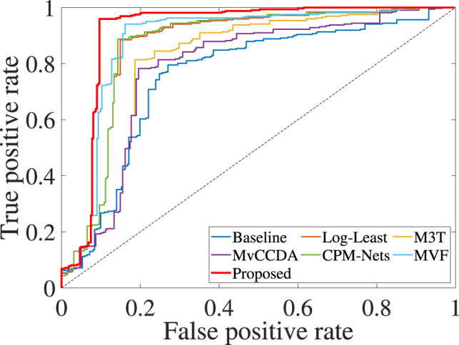
The ROC curves of all methods on the COVID-19 data set.

First, the proposed framework obtained the best classification and regression performance on the COVID-19 data set, followed by Log-Least, MVF, M3T, CPM-Nets, MvCCDA, and Baseline. For example, our framework improved by 9.35% and 17.33% on average, respectively, compared to the best comparison method (i.e., Log-Least) and the worse comparison method (i.e., Baseline), in terms of all classification evaluation metrics. Moreover, the proposed framework obtained the best correlation coefficient, i.e., with the improvement of 3.30%, 6.20%, 7.90%, 8.80%, 15.70%, and 16.70%, respectively, compared to MVF, CPM-Nets, Log-Least, M3T, MvCCDA, and Baseline. Furthermore, the proposed framework achieved the lowest RMSE (e.g., 3.56). The reason is that our proposed framework solved the issues, such as the class imbalance, the HDLSS data, and the slight difference between mild cases and severe cases on the chest CT images. On the contrary, the comparison methods only explored a part of the aforementioned issues.

Second, the dimensionality reduction methods (such as M3T, MvCCDA, Log-Least, CPM-Nets, and MVF) outperformed Baseline, which conducts joint classification and regression on the original data. For example, Log-Least improved by 7.98% on average, compared to Baseline, in terms of all three classification metrics. Hence, in the imbalanced data set, feature selection is still important for dealing with high-dimensional data.

2.6. Discussion

In the section, we evaluated the effectiveness of our proposed framework, i.e., the effectiveness of the data augmentation in Fig. 3, Fig. 4, the interpretability of the selected feature by our framework in Table 4, and the parameters’ sensitivity and the convergence analysis of our proposed framework in Fig. 5.

Fig. 3.

Classification accuracy of all comparison methods with the data augmentation step on the COVID-19 data set. It is noteworthy that the results of Proposed is exactly same as the results of Proposed in Table 3.

Fig. 4.

Classification accuracy of the proposed framework and the proposed framework without the data augmentation step (i.e., Proposed-w/o) on the COVID-19 data set.

Table 4.

The distribution of top ROIs selected by the proposed framework.

Hu ranges	Left lung (6)	Right lung (9)
[-$\infty$,-700]	1	1
[-700,-500]	2	2
[-500,-200]	2	4
[-200,50]	0	2
[50, $\infty$]	1	0

Fig. 5.

The variations of the classification accuracy (left) and the correlation coefficient (middle) of the proposed framework with different parameters’ setting, and the variations of the objective function values (right) of the proposed framework at different iteration times, on the COVID-19 data set.

2.6.1. Class imbalance effectiveness

First, among all methods, the proposed framework and Log-Least take into account the class imbalance problem. Based on Table 1, Table 2, Table 3 where two synthetic data sets are balanced data sets and the COVID-19 data set has the class imbalance problem. As a result, our proposed framework achieved the best performance, while Log-Least achieved the second-best on the COVID-19 data set, but ranked top 4 on two synthetic data sets. For example, Log-Least decreased by 8.85% on average on two synthetic data sets, but increased by around 0.27% on the COVID-19 data set, compared to MVF, in terms of all classification evaluation metrics. This shows the importance of the data augmentation technique for imbalanced data sets.

Second, we employed the SMOTE technique in our framework to all comparison methods, and then listed the classification performance in Fig. 3. As a consequence, all comparison methods improved the classification performance, compared to their classification performance reported in Table 3. For example, MVF achieved the maximal improvement, i.e., 7.15% and Log-Least obtained the minimal improvement, i.e., 2.57%. However, their classification performance is still worse than the performance of our proposed framework. In particular, although Log-Least used a sparse method to deal with the class imbalance problem and has been found to outperform other comparison methods on the imbalanced data set (i.e., the COVID-19 data set), it still improved the classification accuracy by 0.44% with the augmented minority samples. The possible reason is that Log-Least uses the sparse method to reduce the number of majority samples, thus it is difficult to construct effective classification models with limited samples. On the contrary, the SMOTE used in our framework augments the minority samples to have enough training samples which guarantee to produce effective classification models.

Third, we conducted the classification task with our proposed framework without the data augmentation step (i.e., Proposed-w/o) to evaluate the effectiveness of our proposed MM-SVM method in Fig. 4. Based on the results, the classification accuracy Proposed-w/o outperformed the performance of all comparison methods in Table 3, where all comparison methods did not take into account the class imbalance problem. For example, the proposed framework improved by around 6.29%, compared to Proposed-w/o, in terms of three classification evaluation metrics. Proposed-w/o improved by 3.33% on average, compared to the best comparison methods in Table 3, in terms of three classification evaluation metrics. This implied that (1) the data augmentation is necessary for dealing with the imbalanced data set and (2) the proposed framework is better than all comparison methods even though only considering the issues such as the slight appearance difference between mild cases and severe cases, the HDLSS data, and the interpretability.

2.6.2. Interpretability of top selected regions

We listed the top selected features (i.e., the chest ROIs) by our proposed framework in Table 4, which could benefit the clinicians for the practical applications, e.g., improving the efficiency and the effectiveness of the disease diagnosis and reducing the clinicians’ workloads. To this end, we first calculated the times of each feature selected by our proposed framework in all 100 experiments, i.e., repeating the 10-fold cross-validation scheme 10 times, and then selected 15 features (i.e., chest ROIs) whose frequency was larger than 95 out of 100.

Most of the top features (i.e., 9 of 15) were in the right lung and 10 of 15 top ROIs were in the HU range of $[-700,-200]$. This shows that (1) the COVID-19 has more influence in the right lung than the influence in the left lung and (2) the severity of the COVID-19 may be related to the regions of the ground glass opacity whose HU ranges are between −700 and -200, as shown in previous literature (Tang, et al., 2020, Zhu, et al., 2021).

2.6.3. Sensitivity of parameters

The previous study has demonstrated that the SVM framework is very sensitive to the selection of the parameters $C_1$ and $C_2$ (Cortes & Vapnik, 1995), so do they in this work. We did not report such results because it is not the main contribution of this work.

Based on the results in Fig. 5, the proposed framework is sensitive to the selection of the parameters (i.e., $\lambda$ and $\rho$). However, it is easy for our framework to obtain good performance. For example, the proposed framework obtained good performance in terms of classification accuracy and correlation coefficient, on the COVID-19 data set with $(\lambda =1,\rho =2)$ and $(\lambda =3,\rho =2)$, respectively.

2.6.4. Convergence analysis

In Section 1.3.4, we theoretically proved the convergence of our proposed Algorithm 1 to optimize the objective function in Eq. (8). In this section, we investigated the variations of the objective function values of Eq. (8) with different iteration times. To this end, we set the stop criteria of our proposed Algorithm 1 as $\frac{|obj(t+1)-obj\left(t\right)|}{obj\left(t\right)}\le 10^{-4}$, where $obj\left(t\right)$ denotes the objection function value in the $t$th iteration.

As a result, our proposed Algorithm 1 ran a few iteration times to reach the convergence. That is, our proposed optimization method can efficiently achieve convergence.

3. Conclusion

In this study, we proposed a novel framework to conduct joint disease diagnosis and conversion time prediction. To this end, we conducted hierarchical segmentation on the chest CT scans as well as used the common information across tasks and modalities to detect the slight appearance difference between mild cases and severe cases, employed the oversampling method to augment the minority samples for solving the class imbalance problem, and designed a novel multi-task multi-modality SVM method to deal with the issue of the HDLSS data and achieve the interpretability at the same time. Experimental results on both synthetic data sets and the real COVID-19 data set verified the effectiveness of the proposed framework, compared to the state-of-the-art methods.

In this study, we only focused on binary classification, i.e., severe cases vs. mild cases. In our future work, we plan to conduct a multi-class classification of the COVID-19 disease. Moreover, we also plan to design new registration techniques to align the longitudinal images of the same patients, and thus providing accurate measurement of the local infection changes.

CRediT authorship contribution statement

Rongyao Hu: Conceptualization, Methodology, Formal analysis, Supervision, Project administration, Funding acquisition, Writing – review & editing. Jiangzhang Gan: Data curation, Resources, Supervision, Project administration. Xiaofeng Zhu: Software, Formal analysis, Writing – review & editing. Tong Liu: Data curation, Investigation, Project administration. Xiaoshuang Shi: Formal analysis, Resources, Project administration.

Declaration of Competing Interest

The authors declare that they have no known competing financial interests or personal relationships that could have appeared to influence the work reported in this paper.

References

- Bai Xiang, Fang Cong, Zhou Yu, Bai Song, Liu Zaiyi, Xia Liming, et al. 2020. Predicting COVID-19 malignant progression with AI techniques. [DOI] [PMC free article] [PubMed] [Google Scholar]
- Bezdek James C., Hathaway Richard J. Convergence of alternating optimization. Neural, Parallel & Scientific Computations. 2003;11(4):351–368. [Google Scholar]
- Bottou Léon, Lin Chih-Jen. Support vector machine solvers. Large Scale Kernel Machines. 2007;3(1):301–320. [Google Scholar]
- Boyd, Vandenberghe, Faybusovich Convex optimization. IEEE Transactions on Automatic Control. 2006;51(11):1859. [Google Scholar]
- Chawla Nitesh V, Bowyer Kevin W, Hall Lawrence O, Kegelmeyer W Philip. Smote: synthetic minority over-sampling technique. Journal of Artificial Intelligence Research. 2002;16:321–357. [Google Scholar]
- Chimmula Vinay Kumar Reddy, Zhang Lei. Time series forecasting of COVID-19 transmission in Canada using lstm networks. Chaos, Solitons & Fractals. 2020 doi: 10.1016/j.chaos.2020.109864. [DOI] [PMC free article] [PubMed] [Google Scholar]
- Cortes Corinna, Vapnik Vladimir. Support-vector networks. Machine Learning. 1995;20(3):273–297. [Google Scholar]
- Fan Deng-Ping, Zhou Tao, Ji Ge-Peng, Zhou Yi, Chen Geng, Fu Huazhu, et al. Inf-net: Automatic COVID-19 lung infection segmentation from ct images. IEEE Transactions on Medical Imaging. 2020 doi: 10.1109/TMI.2020.2996645. [DOI] [PubMed] [Google Scholar]
- Fang Mengjie, He Bingxi, Li Li, Dong Di, Yang Xin, Li Cong, et al. CT radiomics can help screen the coronavirus disease 2019 (COVID-19): A preliminary study. Science China. Information Sciences. 2020;63(7) [Google Scholar]
- Galar Mikel, Fernandez Alberto, Barrenechea Edurne, Bustince Humberto, Herrera Francisco. A review on ensembles for the class imbalance problem: bagging-, boosting-, and hybrid-based approaches. IEEE Transactions on Systems, Man, and Cybernetics, Part C (Applications and Reviews) 2011;42(4):463–484. [Google Scholar]
- Gan Jiangzhang, Peng Ziwen, Zhu Xiaofeng, Hu Rongyao, Ma Junbo, Wu Guorong. Brain functional connectivity analysis based on multi-graph fusion. Medical Image Analysis. 2021;71 doi: 10.1016/j.media.2021.102057. [DOI] [PMC free article] [PubMed] [Google Scholar]
- Gill Philip E., Robinson Daniel P. A primal-dual augmented Lagrangian. Computational Optimization and Applications. 2012;51(1):1–25. [Google Scholar]
- Guan Wei-jie, Ni Zheng-yi, Hu Yu, Liang Wen-hua, Ou Chun-quan, He Jian-xing, et al. Clinical characteristics of coronavirus disease 2019 in China. New England Journal of Medicine. 2020 doi: 10.1056/NEJMoa2002032. [DOI] [PMC free article] [PubMed] [Google Scholar]
- Hamzah FA Binti, Lau C, Nazri H, Ligot DV, Lee G, Tan CL, et al. Coronatracker: worldwide COVID-19 outbreak data analysis and prediction. Bull World Health Organ. 2020;1:32. [Google Scholar]
- Hao Shijie, Zhou Yuan, Guo Yanrong. A brief survey on semantic segmentation with deep learning. Neurocomputing. 2020 doi: 10.1016/j.neucom.2019.11.118. [DOI] [Google Scholar]
- He Haibo, Garcia Edwardo A. Learning from imbalanced data. IEEE Transactions on Knowledge and Data Engineering. 2009;21(9):1263–1284. [Google Scholar]
- Hsieh Cho-Jui, Chang Kai-Wei, Lin Chih-Jen, Keerthi S Sathiya, Sundararajan Sellamanickam. ICML. 2008. A dual coordinate descent method for large-scale linear SVM; pp. 408–415. [Google Scholar]
- Hu Zixin, Ge Qiyang, Jin Li, Xiong Momiao. 2020. Artificial intelligence forecasting of covid-19 in China. arXiv preprint arXiv:2002.07112. [DOI] [PMC free article] [PubMed] [Google Scholar]
- Hu Rongyao, Peng Ziwen, Zhu Xiaofeng, Gan Jiangzhang, Zhu Yonghua, Ma Junbo, et al. Multi-band brain network analysis for functional neuroimaging biomarker identification. IEEE Transactions on Medical Imaging. 2021 doi: 10.1109/TMI.2021.3099641. [DOI] [PMC free article] [PubMed] [Google Scholar]
- Kang Hengyuan, Xia Liming, Yan Fuhua, Wan Zhibin, Shi Feng, Yuan Huan, et al. Diagnosis of coronavirus disease 2019 (covid-19) with structured latent multi-view representation learning. IEEE Transactions on Medical Imaging. 2020 doi: 10.1109/TMI.2020.2992546. [DOI] [PubMed] [Google Scholar]
- Li Xuelong, Chen Mulin, Nie Feiping, Wang Qi. AAAI, Vol. 31. 2017. A multiview-based parameter free framework for group detection; pp. 4147–4153. [Google Scholar]
- Liu Xu-Ying, Wu Jianxin, Zhou Zhi-Hua. Exploratory undersampling for class-imbalance learning. IEEE Transactions on Systems, Man and Cybernetics, Part B (Cybernetics) 2008;39(2):539–550. doi: 10.1109/TSMCB.2008.2007853. [DOI] [PubMed] [Google Scholar]
- Longadge Rushi, Dongre Snehalata. 2013. Class imbalance problem in data mining review. arXiv preprint arXiv:1305.1707. [Google Scholar]
- Ouyang Xi, Huo Jiayu, Xia Liming, Shan Fei, Liu Jun, Mo Zhanhao, et al. Dual-sampling attention network for diagnosis of COVID-19 from community acquired pneumonia. IEEE Transactions on Medical Imaging. 2020 doi: 10.1109/TMI.2020.2995508. [DOI] [PubMed] [Google Scholar]
- Pedregosa Fabian, Varoquaux Gaël, Gramfort Alexandre, Michel Vincent, Thirion Bertrand, Grisel Olivier, et al. Scikit-learn: Machine learning in python. Journal of Machine Learning Research. 2011;12:2825–2830. [Google Scholar]
- Peng Liang, Kong Fei, Liu Chongzhi, Kuang Ping. Robust and dynamic graph convolutional network for multi-view data classification. The computer Journal. 2021 [Google Scholar]
- Qi Xiaolong, Jiang Zicheng, Yu Qian, Shao Chuxiao, Zhang Hongguang, Yue Hongmei, et al. Machine learning-based CT radiomics model for predicting hospital stay in patients with pneumonia associated with SARS-CoV-2 infection: A multicenter study. MedRxiv. 2020 doi: 10.21037/atm-20-3026. [DOI] [PMC free article] [PubMed] [Google Scholar]
- Shan Fei, Gao Yaozong, Wang Jun, Shi Weiya, Shi Nannan, Han Miaofei, et al. 2020. Lung infection quantification of COVID-19 in CT images with deep learning. arXiv preprint arXiv:2003.04655. [Google Scholar]
- Shen Heng Tao, Zhu Yonghua, Zheng Wei, Zhu Xiaofeng. Half-quadratic minimization for unsupervised feature selection on incomplete data. IEEE Transactions on Neural Networks and Learning Systems. 2020 doi: 10.1109/TNNLS.2020.3009632. [DOI] [PubMed] [Google Scholar]
- Shi Feng, Wang Jun, Shi Jun, Wu Ziyan, Wang Qian, Tang Zhenyu, et al. Review of artificial intelligence techniques in imaging data acquisition, segmentation and diagnosis for covid-19. IEEE Reviews in Biomedical Engineering. 2020 doi: 10.1109/RBME.2020.2987975. [DOI] [PubMed] [Google Scholar]
- Shi Feng, Xia Liming, Shan Fei, Wu Dijia, Wei Ying, Yuan Huan, et al. 2020. Large-scale screening of covid-19 from community acquired pneumonia using infection size-aware classification. arXiv preprint arXiv:2003.09860. [DOI] [PubMed] [Google Scholar]
- Song Yong Sub, Park Chang Min, Park Sang Joon, Lee Sang Min, Jeon Yoon Kyung, Goo Jin Mo. Volume and mass doubling times of persistent pulmonary subsolid nodules detected in patients without known malignancy. Radiology. 2014;273(1):276–284. doi: 10.1148/radiol.14132324. [DOI] [PubMed] [Google Scholar]
- Tang Zhenyu, Zhao Wei, Xie Xingzhi, Zhong Zheng, Shi Feng, Liu Jun, et al. 2020. Severity assessment of coronavirus disease 2019 (COVID-19) using quantitative features from chest CT images. arXiv preprint arXiv:2003.11988. [Google Scholar]
- Vapnik Vladimir N. An overview of statistical learning theory. IEEE Transactions on Neural Networks. 1999;10(5):988–999. doi: 10.1109/72.788640. [DOI] [PubMed] [Google Scholar]
- Wang Shuai, Kang Bo, Ma Jinlu, Zeng Xianjun, Xiao Mingming, Guo Jia, et al. A deep learning algorithm using CT images to screen for corona virus disease (COVID-19) MedRxiv. 2020 doi: 10.1007/s00330-021-07715-1. [DOI] [PMC free article] [PubMed] [Google Scholar]
- Wang Rong, Nie Feiping, Wang Zhen, Hu Haojie, Li Xuelong. Parameter-free weighted multi-view projected clustering with structured graph learning. IEEE Transactions on Knowledge and Data Engineering. 2019;32(10):2014–2025. [Google Scholar]
- Wu Xiangjun, Hui Hui, Niu Meng, Li Liang, Wang Li, He Bingxi, et al. Deep learning-based multi-view fusion model for screening 2019 novel coronavirus pneumonia: A multicentre study. European Journal of Radiology. 2020 doi: 10.1016/j.ejrad.2020.109041. [DOI] [PMC free article] [PubMed] [Google Scholar]
- Xie Weiyi, Jacobs Colin, Charbonnier Jean-Paul, van Ginneken Bram. Relational modeling for robust and efficient pulmonary lobe segmentation in ct scans. IEEE Transactions on Medical Imaging. 2020 doi: 10.1109/TMI.2020.2995108. [DOI] [PMC free article] [PubMed] [Google Scholar]
- You Xinge, Xu Jiamiao, Yuan Wei, Jing Xiao-Yuan, Tao Dacheng, Zhang Taiping. Multi-view common component discriminant analysis for cross-view classification. Pattern Recognition. 2019;92:37–51. [Google Scholar]
- Yuan Changan, Zhong Zhi, Lei Cong, Zhu Xiaofeng, Hu Rongyao. Adaptive reverse graph learning for robust subspace learning. Information Processing & Management. 2021 doi: 10.1016/j.ipm.2021.102733. [DOI] [Google Scholar]
- Zhang Zheng, Lai Zhihui, Huang Zi, Wong Wai Keung, Xie Guo-Sen, Liu Li, et al. Scalable supervised asymmetric hashing with semantic and latent factor embedding. IEEE Transactions on Image Processing. 2019;28(10):4803–4818. doi: 10.1109/TIP.2019.2912290. [DOI] [PubMed] [Google Scholar]
- Zhang Zheng, Liu Li, Shen Fumin, Shen Heng Tao, Shao Ling. Binary multi-view clustering. IEEE Transactions on Pattern Analysis and Machine Intelligence. 2019;41(7):1774–1782. doi: 10.1109/TPAMI.2018.2847335. [DOI] [PubMed] [Google Scholar]
- Zhang Daoqiang, Shen Dinggang, Alzheimer’s Disease Neuroimaging Initiative, et al. Multi-modal multi-task learning for joint prediction of multiple regression and classification variables in Alzheimer’s disease. NeuroImage. 2012;59(2):895–907. doi: 10.1016/j.neuroimage.2011.09.069. [DOI] [PMC free article] [PubMed] [Google Scholar]
- Zhu Yonghua, Ma Junbo, Yuan Changan, Zhu Xiaofeng. Interpretable learning based dynamic graph convolutional networks for alzheimers disease analysis. Information Fusion. 2021 doi: 10.1016/j.inffus.2021.07.013. [DOI] [Google Scholar]
- Zhu Xiaofeng, Song Bin, Shi Feng, Chen Yanbo, Hu Rongyao, Gan Jiangzhang, et al. Joint prediction and time estimation of COVID-19 developing severe symptoms using chest CT scan. Medical Image Analysis. 2021;67 doi: 10.1016/j.media.2020.101824. [DOI] [PMC free article] [PubMed] [Google Scholar]
- Zhu Xiaofeng, Yang Jianye, Zhang Chengyuan, Zhang Shichao. Efficient utilization of missing data in cost-sensitive learning. IEEE Transactions on Knowledge and Data Engineering. 2019 doi: 10.1109/TKDE.2019.2956530. [DOI] [Google Scholar]
- Zhu Xiaofeng, Zhang Shichao, Zhu Yonghua, Zhu Pengfei, Gao Yue. Unsupervised spectral feature selection with dynamic hyper-graph learning. IEEE Transactions on Knowledge and Data Engineering. 2020 doi: 10.1109/TKDE.2020.3017250. [DOI] [Google Scholar]