Abstract
Arterial stiffness is an important biomarker for many cardiovascular diseases. Shear wave elastography is a recent technique aimed at estimating local arterial stiffness using guided wave inversion (GWI), i.e. matching the computed and measured wave dispersion. This paper develops and validates a new GWI approach by synthesizing various recent observations and algorithms: (a) refinements to signal processing to obtain more accurate experimental dispersion curves; (b) an efficient forward model to compute theoretical dispersion curves for immersed, incompressible cylindrical waveguides; (c) an optimization framework based on the recent observation that the measured dispersion curve is multimodal, i.e. it matches for not one but two different wave modes in two different frequency ranges. The resulting inversion approach is validated using extensive experimental data from rubber tube phantoms, not only for modulus estimation but also to simultaneously estimate modulus and wall thickness. The observations indicate that the modulus estimates are best performed with the information on wall thickness. The approach, which takes less than half a minute to run, is shown to be accurate, with the modulus estimated with less than 4% error for 70% of the experiments.
Introduction
Arterial stiffness is a well-known biomarker of early cardiovascular diseases (Palombo and Kozakova 2016, Chirinos et al 2019, Sun 2015). The pulse wave velocity (PWV) is a widely used biomarker for arterial stiffness (Vlachopoulos et al 2010, Laurent et al 2006, Chirinos et al 2019, McGarry et al 2016, Segers et al 2020). The PWV is currently measured by evaluating the time delay between the pressure waveforms measured using tonometry at the carotid and femoral arteries and using an estimated travel distance (Kullo and Malik 2007). However, given the approximate and average nature of the resulting PWV estimation, there is a concerted effort to estimate localized arterial stiffness, e.g. that of the carotid artery. This has been done using measurements of vessel distension with high frame rate ultrasound imaging (Luo et al 2009, Vappou et al 2010, Luo et al 2012, Parameswaran et al 2019, Marais et al 2019).
Shear wave elastography (SWE) of the arterial stiffness using acoustic radiation force (ARF) has shown to be a promising tool to estimate the stiffness of carotid artery (Couade et al 2010, Bernal et al 2011, Pruijssen et al 2020). The main idea of arterial SWE is to use ARF excitation to generate waves propagating within the arterial walls, and use the characteristics of the propagating waves to estimate the arterial stiffness.
The main approach to estimate arterial stiffness from the measured response is through inversion, i.e. iteratively changing the properties of a model to minimize the difference between simulated and measured dispersion curves that represent the variation of phase velocity as a function of frequency. These curves reflect how the time-domain waveform distorts as it propagates along the artery. The measured dispersion curve is obtained from processing the wall motion data acquired using high frame rate ultrasound imaging. The simulated dispersion curve is obtained through a forward model, i.e. analytical or computational model that can predict the wave dispersion given the arterial material and geometric properties.
Various forward models have been developed to compute wave dispersion in arteries. Early models were focused on the simplification of geometric complexities leading to analytical solutions, with later models focused on both analytical and computational techniques. Some of the existing analytical models include, plate (Couade et al 2010, Bernal et al 2011, Nguyen et al 2011, Widman et al 2015, Jang et al 2015, Widman et al 2016, Maksuti et al 2016, Li et al 2017a), hollow tube (Zhang et al 2005, Flamini et al 2015), and fluid-filled tube (Flamini et al 2015, Lin et al 2015). A more detailed three-dimensional finite element model is utilized in (Dutta et al 2015). In (Astaneh et al 2017) and (Roy and Guddati 2021), a waveguide model based on semi-analytical finite element (SAFE) methods was developed to capture the fully three-dimensional wave propagation in a fluid-filled immersed tube, but with a significantly reduced computational cost without sacrificing accuracy. Through a validation exercise in (Astaneh et al 2017), we found that the experimental dispersion curve matches not with a single simulated curve, but multiple curves depending on the frequency range. The goal of this paper is to build on this observation and develop and validate inversion approaches to estimate the arterial modulus.
Most of the existing work focused on estimating the shear modulus to characterize the arterial stiffness (Couade et al 2010, Bernal et al 2011, Nguyen et al 2011, Widman et al 2015, 2016, Maksuti et al 2016, Li et al 2017a). However, it is known that thickness also significantly contributes towards artery stiffness estimation (Maksuti et al 2017, Astaneh et al 2017, Dutta et al 2015). Because it is small, the thickness, which is often measured using ultrasound B-mode images, may not always be accurate. Thus, if possible, it would be desirable to estimate the thickness in addition to modulus, from the wave dispersion properties. Exploring this possibility is a secondary goal of the current study.
The outline of the paper is as follows. After summarizing the basic idea of shear wave elastography for arteries, we describe the data acquisition and processing to obtain the experimental dispersion curve, which includes a summary of recent signal processing refinements. We then focus on the forward model to compute the simulated dispersion curves. In the following section, we discuss the necessary details related to inversion, i.e. parametrization, objective function, and optimization algorithms. The validation study is then presented followed by concluding remarks.
Shear Wave Elastography of Arteries
Given that arterial wall modulus is much higher than the surrounding tissue, a high-frequency pulse from the acoustic radiation force generates waves that are guided along the arterial wall. The dispersion characteristics of the guided waves are used to estimate the arterial modulus and thus the stiffness (Couade et al 2010, Bernal et al 2011). The schematic of the methodology for phantom experiments is shown in Figure 1. The procedure involves two major steps:
Data Acquisition and Signal Processing: The shear waves are generated inside the tube and the resulting wave propagation response is measured on the top surface along the axis of the tube as shown in Fig. 1(a). The recorded spatiotemporal response (Fig. 1(b)) is transformed into the frequency-wavenumber (f-k) domain through a two-dimensional Fast Fourier Transformation (2D FFT), as shown in Fig. 1(c). The peaks in the f-k data are identified and plotted as a dispersion curve, i.e. plot of phase velocity (cp = 2πf/k)vs. f (Fig. 1(d)).
Inversion through Optimization: The last major step is to back-calculate the properties of the tube through matching the measured dispersion curve with the simulated dispersion curve by iteratively changing the properties of the tube (Fig. 1(e)). The simulated dispersion curves are calculated using an analytical or computational forward model (Fig. 1(f)). The back-calculation (inversion) is performed through optimization, i.e. minimizing the difference between the measured and simulated dispersion curves.
Figure 1.
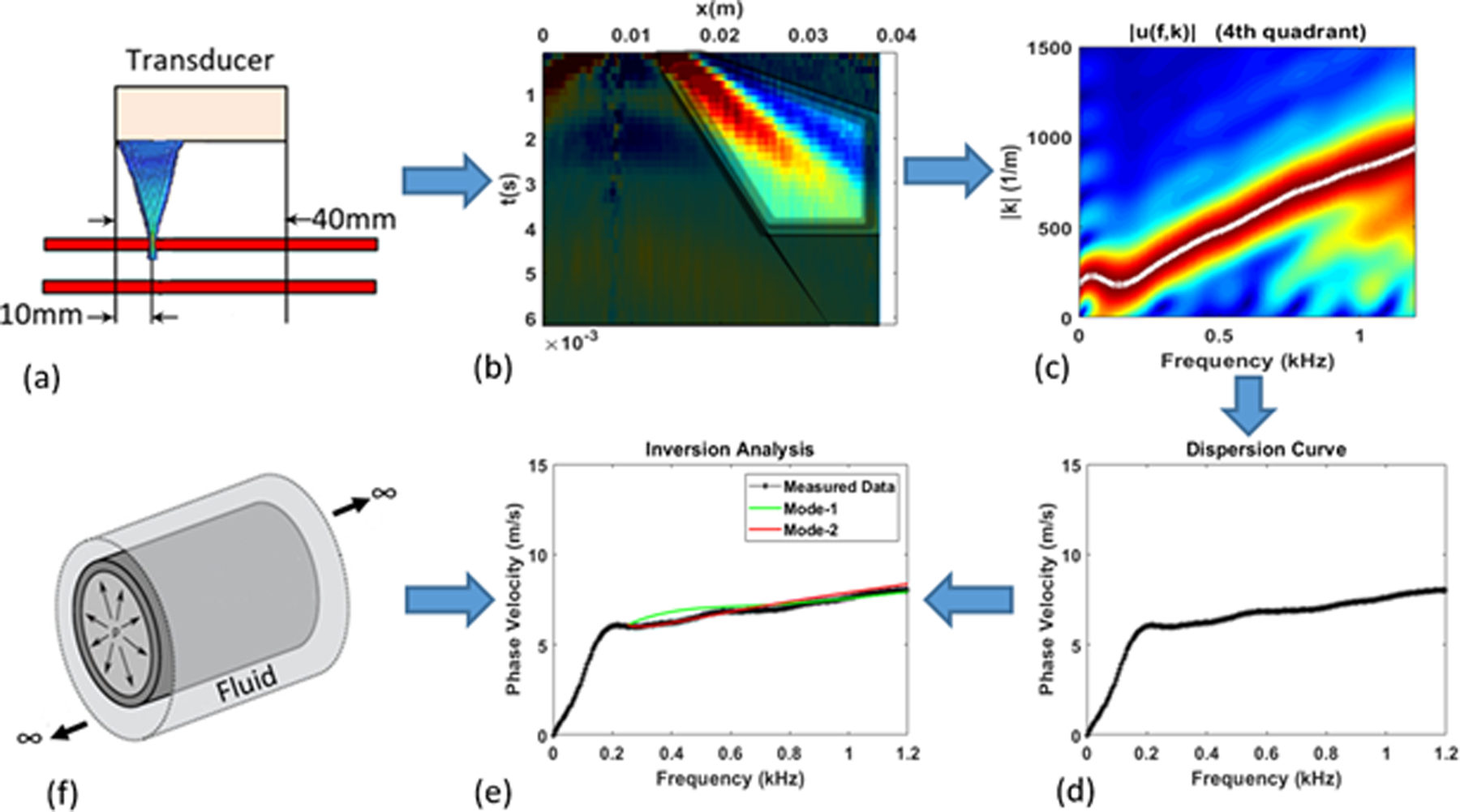
(a) Data Acquisition, (b) Data processing, (c) Frequency-wavenumber plot, (d) Measured dispersion curve, (e) Matching of measured and simulated dispersion curves to back-calculate material and geometric properties, (f) Forward model.
Data Acquisition and Signal Processing
Experimental set-up
Shear wave elastography experiments using Acoustic Radiation Force (ARF) were performed on ten artery mimicking urethane rubber tubes (VytaFlex 10, Smooth-On, Inc., Macungie, PA). The tubes were made in a custom-made mold that could accommodate 3 tubes for a given batch of the rubber. To obtain 10 tubes, four different batches were made as two tubes were damaged in removal from the mold. The tubes are filled with and submerged in water, to simulate blood and surrounding tissue respectively. The inner radius of the tubes is 3 mm and the wall thickness is 1 mm. The schematic of the ARF experimental setup is shown in Figure 2. In these experiments a Verasonics V1 system (Verasonics, Inc., Kirkland, WA) was used equipped with a linear array transducer (L7-4, Philips Healthcare, Andover, MA). The 128 element transducer has elements with 0.283 mm width, 0.025 mm kerf, 7 mm height, and an elevation focus near 25 mm. An ARF push is applied at the x = 10 mm location in Fig. 2(a), and the vertical motion of the wall is measured at the top of the tube along the axis, from x = 10–40 mm. A 400 μs toneburst at 4.09 MHz was used. The push beam used 64 elements of an ultrasound transducer and was focused at 20 mm (F-number = 1, where F-number is the ratio of the focal depth to the aperture width). Plane wave imaging with 5 MHz pulses was used at a pulse repetition period of 80 μs for a pulse repetition frequency of 12.5 kHz. The particle velocity of the wall was estimated from the acquired in-phase/quadrature (IQ) data using an autocorrelation method (Kasai et al 1985). To average the inhomogeneity associated with fabrication, a total of 6 configurations are tested (by performing 60° rotations around the axis). The response is obtained for 10 separate ARF excitations for each of the 6 configurations, leading to 60 data sets for each tube.
Figure 2.
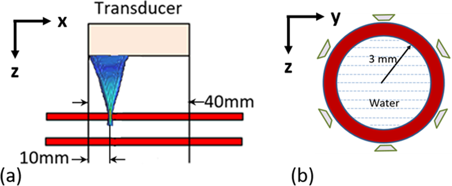
Schematic of experimental setup for measuring wall motion. (a) shows the longitudinal view of the tube and ARF transducer, while (b) shows the cross-section of the tube and the six angles used for ARF excitation and acquisition.
To facilitate the validation of the proposed inversion procedure, the material for each tube was tested mechanically, with of Hyper-Frequency Viscoelastic Spectroscopy (Hadj Henni et al 2011) (Rheospectris C500+, Rheolution, Inc., Montreal, Quebec, Canada), resulting in the storage, Gs(ω), and loss, Gl(ω), moduli for each of the tubes. The moduli were measured from 10–2000 Hz in 10 Hz increments. For each batch of rubber, three cylindrical samples for testing were created when making the tubes. The mean of 3 or 4 acquisitions for each sample were calculated for validation. These results are shown in Figure 3, which will be utilized later in the validation section.
Figure 3.
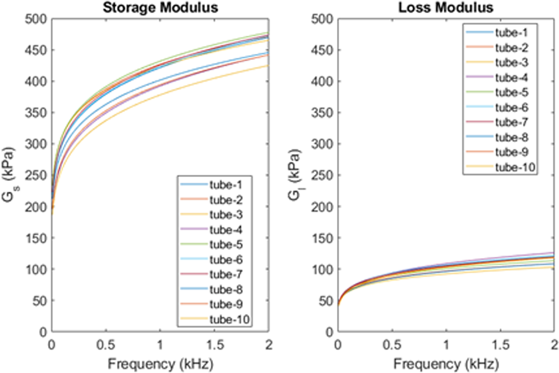
Material properties from Rheospectris experiments.
Data processing
Data processing is performed on the wall motion data first in the spatial-temporal domain. The standard approach is to isolate the right propagating wave as shown in Figure 4. In the proposed approach, we consider only the dominating part of the right propagating region as shown in Figure 5. Specifically, we added a few windowing boundaries to obtain the dispersion curves that are important for inversion. The first windowing boundary, which we call the lower-cut, sets the lower limit on the phase velocity. The second boundary is called the upper cut, as it sets the upper limit on the phase velocity. These lower and upper cuts partially remove the high frequency noise, especially farther from the load at early times, as well as addresses the low signal-to-noise ratio at later times. Finally, the signal is truncated after a maximum time (T-max) to avoid any reflections from the edges of the tube. We consider the resulting trapezoidal region after applying a gradual Gaussian windowing outside these boundaries. The smooth change in the signal amplitude to zero eliminates the spurious Gibbs ringing in the f-k domain. To this end, a Gaussian smoothing function of the following form is used.
| (1) |
Figure 4.
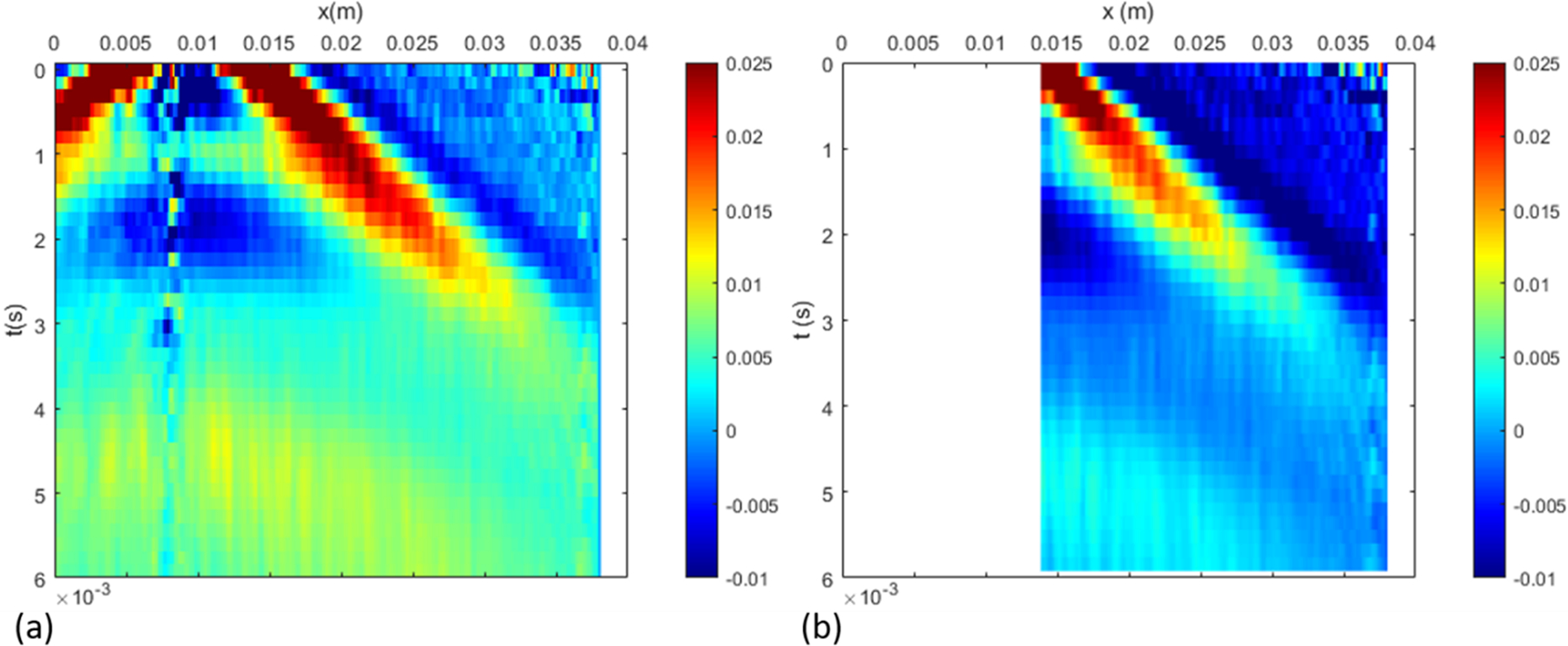
Standard approach for data processing: (a) is the actual measured data in space-time, which is curtailed on the left to focus on the right-propagating waves (b).
Figure 5.
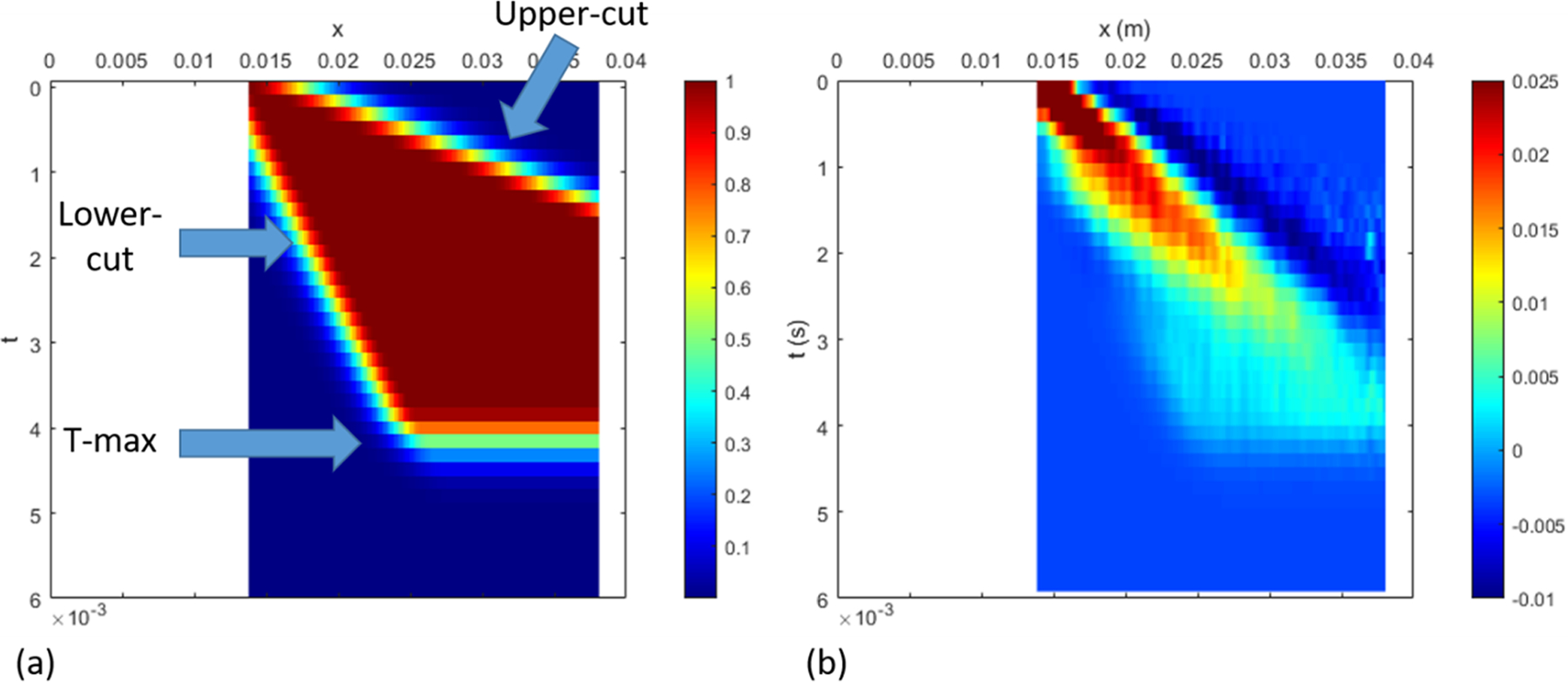
Proposed approach for data processing: In addition to the standard approach in the previous figure, additional windowing is applied to ensure that the dispersion curves are best captured within the range of expected phase velocity. The upper cut sets the upper limit to the phase velocity, the lower cut sets a lower limit, while curtailing in time ensures that the reflections from the boundary does not pollute the dispersion curves.
In the above, the parameter α controls the smoothing rate. The parameters xmax and tmax are the maximum values of x and t in the data, and are utilized essentially as normalization constants. The values of and are determined based on the slopes of the upper and lower cuts and are given by,
| (2) |
where s is the slope of the cuts. The xshift is the shift value along the x direction as shown in Figure 4. The resulting filter is shown in Figure 5(a).
The data processing parameters that describe the windowing are chosen based on the observed phase velocity ranges from the phantom experiments. We observe the phase velocity ranges between 4 to 10 m/s, therefore we choose the lower-cut slope as 3 m/s and upper-cut slope as 15 m/s. Both lower and upper cuts are originated from the starting point in the space-time domain. For the truncation time (T-max), we examine the time when the response is sufficiently attenuated, and well before any boundary reflections are observed. We also confirmed that perturbation of the signal-processing parameters has minimal effect on the dispersion curves (results are not presented for brevity). The remaining steps for either the standard or modified approach are the following: (a) applying the 2D FFT to transfer the space-time data into the wavenumber-frequency domain and (b) picking the peak values to obtain the phase-velocity dispersion with phase-velocity cp = 2πf/k plotted against frequency f.
Figure 6 illustrates the effect of data processing on the dispersion curve, where the experimental dispersion curves are compared with the expected dispersion curves from the model that will be described below, using the material parameters from Rheospectris measurements (shown in Fig. 3). Figure 6 compares experimental dispersion curves from both regular and modified data processing approaches. Clearly, the data processing modifications bring the experimental dispersion curves much closer to the expected dispersion curves. This improvement in the dispersion curves leads to significant change in the inverted parameters, as discussed in the Validation section.
Figure 6.
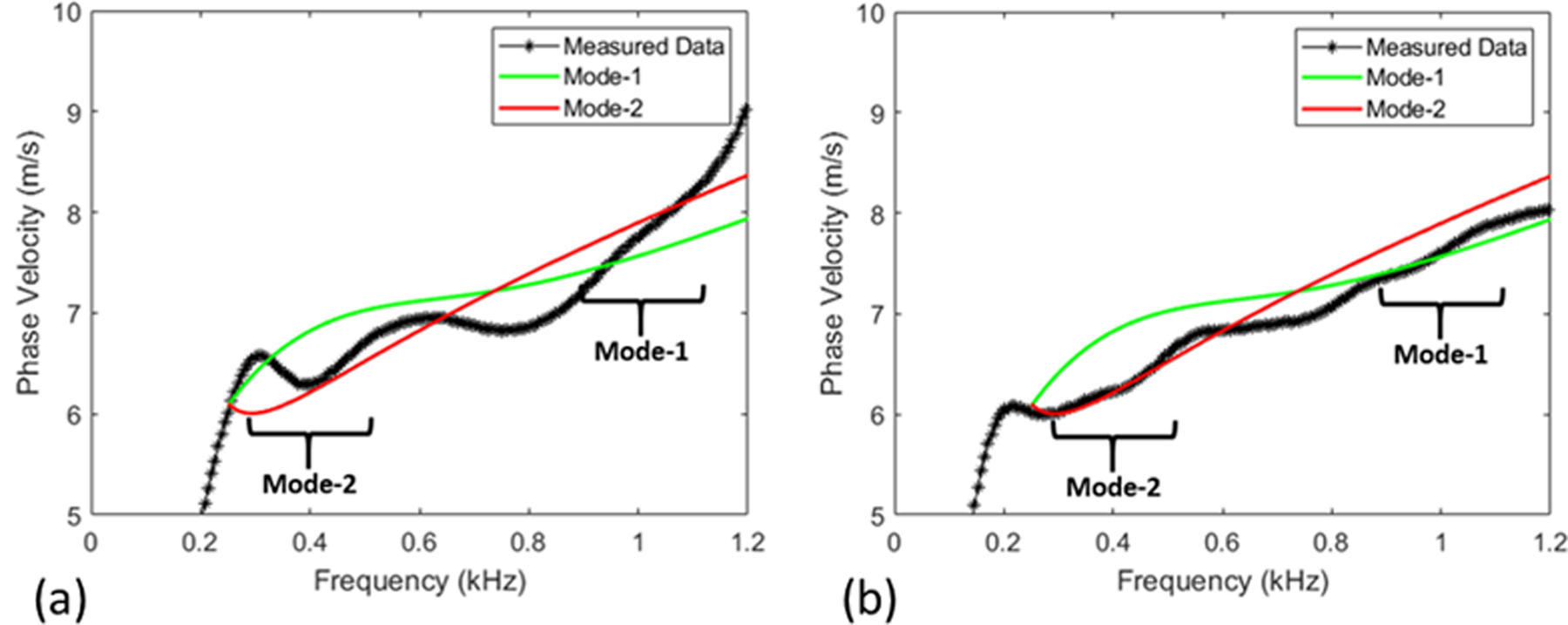
Comparison between simulated and measured dispersion curves with standard processing (a) and refined processing (b). In the two highlighted frequency ranges, the processing refinements result in a better match between measured and simulated dispersion curves.
While other, non-Fourier, methods may be more effective in separating multiple modes with higher fidelity (Tran et al 2014, Kijanka et al 2018, Kijanka and Urban 2021a, 2021b), we emphasize that the current objective is to obtain the most dominant mode in a particular frequency range. The proposed approach is sufficient to this end and alternative methods are not considered at this time; they may be explored in the future, e.g. if the inversion is performed to match multiple modes at the same frequency.
Estimation of Modulus and Thickness
Forward model
To obtain the simulated dispersion curves, the rubber tube is modeled as a cylindrical prism made up of an incompressible elastic material, submerged in an inviscid and incompressible fluid. The idealization of incompressibility is adopted for both the arterial wall and the surrounding fluid because the pressure wave velocity is two orders of magnitude larger than the shear wave velocity; explicit inclusion of compressibility does not change the results much and can lead to unnecessary numerical complications. Further, the tube is assumed to be infinite in length because the experimental data is truncated before any reflections from the tube ends are recorded. Such an assumption facilitates the use of a Semi-Analytical Finite Element (SAFE) formulation, where the discretization is performed in the radial direction, while the analytical expansion is utilized in the axial and azimuthal directions (the reader is referred to (Rose 2014) for detailed explanation and (Nelson et al 1971, Kausel and Peek 1982, Datta et al 1988) for some early work on this topic). The schematic of the geometry is shown in Figure 7 (a), and the summary of the formulation is presented in the remainder of the section.
Figure 7.
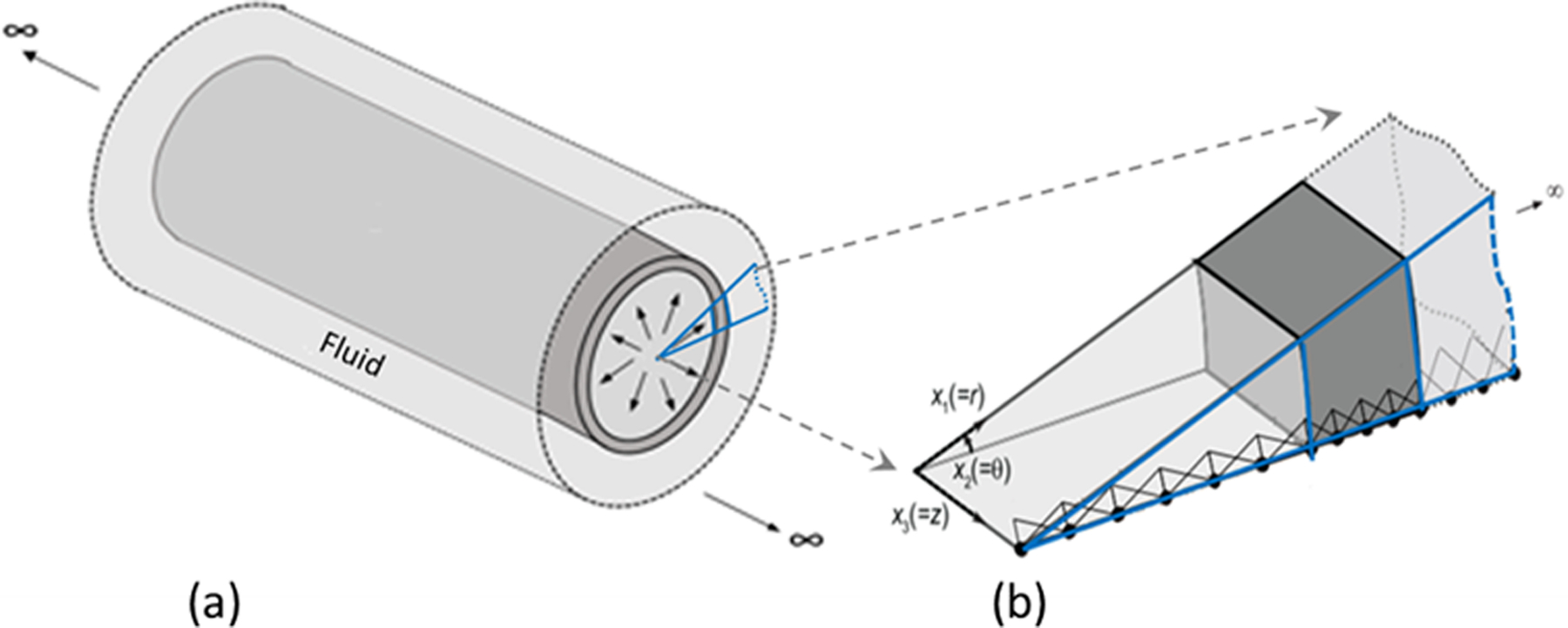
Geometry of the immersed tube (a), and finite element discretization in the radial direction (b). Fourier expansion is used in the axial (x3) and azimuthal (x2) directions.
The tube deformation is governed by the elastodynamic equation,
| (3) |
where, ΩS is the solid domain, σ is the stress, u is the displacement, and ρS is the density of the solid. The operator Lσ is a differential operator representing the symmetric gradient; the details can be found in (Astaneh et al 2017).
Given the incompressible and inviscid nature, the Laplace equation governs the response of the fluid
| (4) |
where ΩF is the fluid domain that encompasses the interior and exterior fluid, p is the fluid pressure, and ρF is the fluid density.
The interface conditions at the solid-fluid interface ΓFS that couples the solid surfaces with both inside and outside fluid regions are,
| (5) |
| (6) |
Here, ns and nF are the unit vectors in the solid and fluid domain respectively, which are in opposite directions. By following the formulation in (Astaneh et al 2017), noting that the geometry and material properties are invariant in the horizontal and azimuthal directions, we consider the SAFE formulation in which the radial direction is discretized with finite elements while analytical expansion is employed for the remaining directions. Specifically, we write the solution in terms of wave modes that are harmonic in time, axial direction, z, and azimuthal direction, θ. Linear finite element discretization is utilized in the radial direction as shown in Fig. 7 (b). Putting these ideas together, given the symmetry of the load and thus the response about the r-z plane, the solid displacement and fluid pressures can be written as,
| (7) |
| (8) |
where NS and NF are the finite element shape functions along the radial direction for the solid and fluid domain respectively, n is the index of the azimuthal harmonic, kz is the wavenumber along the axial direction, ω = 2πf is the temporal frequency, and . Substituting (7) and (8) in governing equations (3) and (4), and interface conditions (5) and (6), results in an eigenvalue problem,
| (9) |
where κ is the normalization factor to improve the conditioning of the system. The solid-domain contribution matrices, , , Ms the fluid-domain contribution matrices, , , and the fluid-structure interaction matrix, CSF are defined in (Astaneh et al 2017); they depend on the geometry (inner radius and thickness) and the material properties (densities and shear modulus). The quadratic eigenvalue problem is solved for each frequency ω, to result in the wavenumber kz, resulting in the dispersion relationship. The dispersion curves can either be plotted in kz −ω space, or a plot of phase velocity (cp = ω/kz) vs. cyclic frequency (f = ω/2π). Consistent with the convention followed in experimental data processing (Figure 5), we follow the latter approach.
The intricacies of the forward modeling include (a) treating incompressibility related linear finite element locking through selective reduced integration (Hughes 2000), (b) simulating the unbounded exterior with perfectly matched discrete layers (Savadatti and Guddati 2010), and (c) normalization to improve the conditioning in the limit of incompressibility (Roy and Guddati 2021). Further details can be found in (Roy and Guddati 2021), where the results from the forward model are compared with the reference solution obtained through convergence analysis (the reference solution is obtained using discretization with highly accurate 5-noded finite elements (Astaneh et al 2017).
Before moving on to inversion, we emphasize that the forward model captures fully three-dimensional wave propagation in the artery. The simulation is simplified mainly due to the simplicity of the tube geometry, allowing the use of SAFE formulation to reduce the computational effort significantly, thus enabling us to use the existing in-house code (Vaziri Astaneh and Guddati 2017) with the minor modifications for the incompressible waveguides and then the off-the-shelf iterative optimization algorithms to estimate the material properties, which is described in the next section.
Inversion through Optimization
Our main goal is to estimate the shear modulus of the artery given the radius and wall thickness. Looking ahead to in vivo application of methodology, we observe that the wall thickness, which is obtained from B-mode images, may not be accurately measured (because the thickness is just a few pixels wide). Given this, we add to our objective the case of simultaneous estimation of shear modulus and wall thickness for known radius of the tube. It is expected from wave physics that the phase velocity will be influenced by both the shear modulus and thickness, making this a plausible goal (we also confirmed that thickness is an influential parameter through sensitivity analysis presented later). Further, at this stage, we assume that the time/frequency dependence of viscoelasticity of the wall is known, and only the scalar measure of the shear modulus is not known. Specifically, we express viscoelastic (complex-valued) shear modulus G(ω) as,
| (10) |
where Gs and Gl are the (real-valued) storage and loss moduli, respectively. Complex-valued F(ω) captures the frequency-dependence of G(ω), while G0 captures the overall magnitude. Without loss of generality, we assume G0 = |G(ω = 20π)|, because ω = 20π is the first frequency point in Rheospectris data (note that this is arbitrary). In our inversion framework, we assume that G0 is the unknown to be determined, while F(ω) is assumed to be known (obtained from the Rheospectris measurements). Inverting for frequency dependency is indeed of interest, but beyond the scope of the current study. Thus, the parameters for our inversion is the wall thickness (h) and the single shear modulus parameter (G0).
The thickness and modulus are estimated by minimizing the difference between the experimentally measured dispersion curves and theoretical dispersion curves computed from the model. Note that there exists a single measured dispersion curve, which is obtained from a single peak in the f-k plot for each frequency (obtaining multiple peaks is not practical due to the low signal-to-noise ratio, especially for in vivo data). As highlighted in (Astaneh et al 2017), this measured dispersion curve does not coincide with a single mode of the simulated dispersion curve, but matches with different modes for different frequency ranges. Specifically, as discussed in (Astaneh et al 2017) and highlighted in Figure 6, the measured dispersion curve matches with flexural mode 2, F(2,1), for 300–500 Hz, while it matches with flexural mode 1, F(1,1), for 900–1200 Hz frequency range. Here, we follow the work of Gazis (Gazis 1959a, 1959b) for the mode numbers notation. In addition, we confirmed this match by comparing with the theoretical dispersion curves of other wave modes that lie in the vicinity (see Figure 8; note that modes with significant evanescence are filtered at low frequencies). As seen in the figure, the L(0,1) mode asymptotically merges with the F(1,1) in the higher frequency range; it is possible that this mode may contribute significantly to the measured dispersion curve for some geometries, material properties and frequency ranges. However, our focus is on frequencies below 1000 Hz, and given that the measured dispersion curve more closely matches with F(2,1) and F(1,1) in this range, we chose to invert by matching with F(2,1) and F(1,1).
Figure 8.
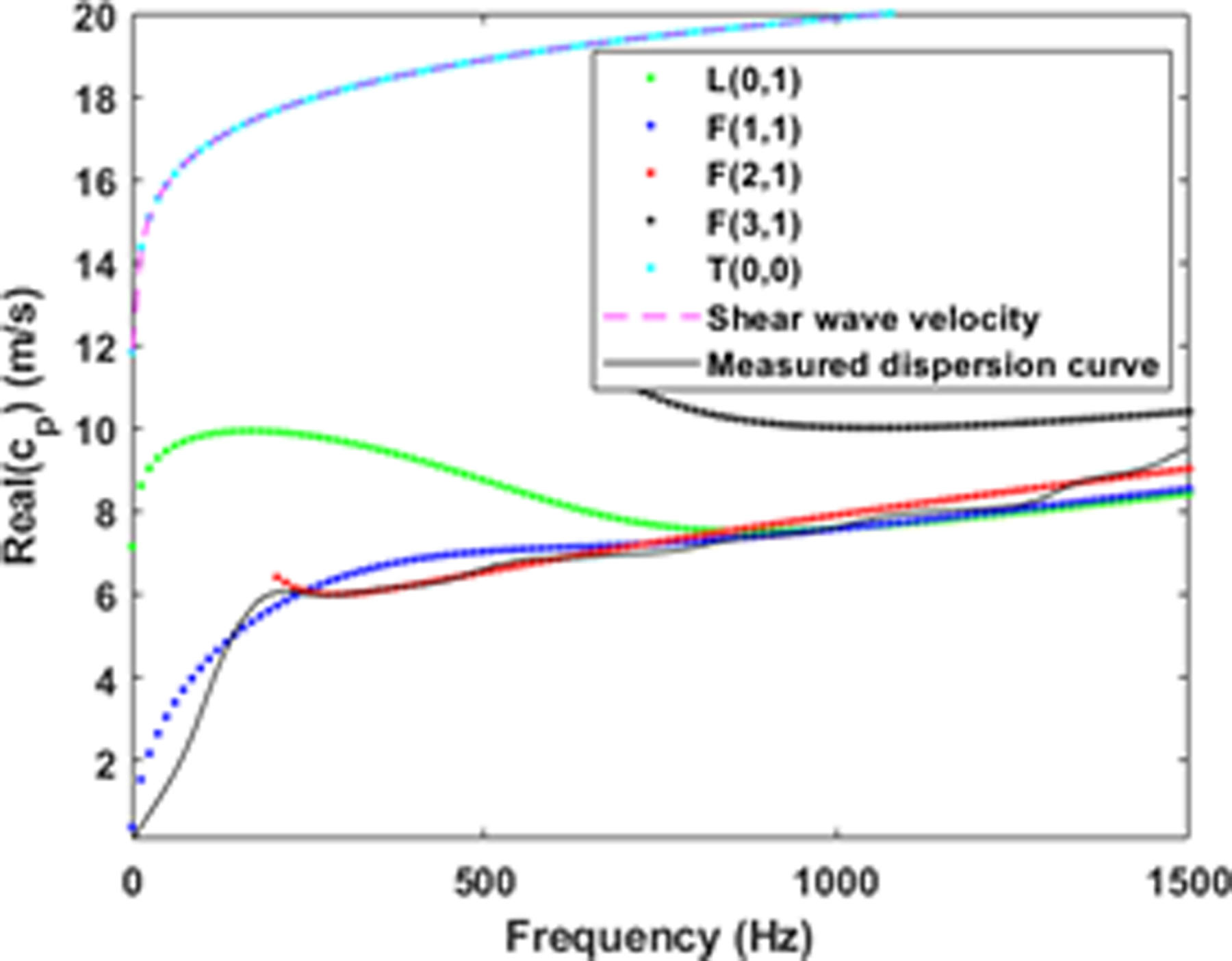
Comparison of the theoretical and measured dispersion curves for the viscoelastic tube
In the inversion analysis, we consider the 900–1000 Hz frequency band for the mode 1 due to the fact that we will not have necessary data beyond 1000 Hz for the in vivo case. Given this observation, we define the objective function as the relative least-squares difference between the dispersion curves:
| (11) |
where, and are the simulated phase velocities corresponding to the modes 1 and 2, respectively, and cm is the phase velocity from the measured data. Consistent with the discussion above, f1 = 300 Hz, f2 = 500 Hz, f3 = 900 Hz, and f4 = 1000 Hz. These frequency ranges may change depending on the geometry and may need to be revisited for in vivo experiments. Note that in the objective function, we consider the phase velocity dispersion instead of the k(ω) dispersion. The reason is that the phase velocity is fairly constant in the considered frequency range unlike the k(ω) dispersion case; matching k(ω) curves will give higher weights to higher-frequency data which is undesirable.
The inverse problem thus involves estimating the parameters G0 and h, given the measured dispersion curve, radius of the tube, and the viscoelastic time-dependency F(ω). This can be performed, e.g. by formulating in a robust PDE constrained optimization framework with explicit formulation of gradient and Hessian, potential with adjoint operators. Such an approach is beneficial for a large parameter space and expensive forward models. However, given that we are inverting for just two parameters and have an extremely efficient forward model, we resort to the black-box optimization algorithms implemented in MATLAB, some of them based on finite-difference gradients.
Inversion Models:
To minimize the objective function in Equation (11), we consider both local and global optimization approaches. While the local optimization gives a minimizer, global optimization removes the possibilities of obtaining a spurious local minimizer. In the local optimization framework, we consider (a) interior point method with the BFGS Hessian (Waltz et al 2006), (b) Nelder-Mead algorithm (Lagarias et al 1998), (c) Non-linear Optimization Mesh Adaptive Direct Search (NOMADS) algorithm (Currie and Wilson 2012). The global optimization algorithms that we consider include (d) Particle-Swarm (Kennedy and Eberhart 1995). Note that except the Nelder-Mead algorithm, all other considered models are constrained optimization and in these cases, we impose box constraints, limiting each parameter to be within ±30% of the mean value. For all the above-mentioned inversion models, we employ the MATLAB optimization toolbox except for the NOMADS algorithm for which we use the available function in (Anon n.d.).
Results and Discussion
Parameter sensitivity
Before embarking on the actual inversion process, we perform formal sensitivity analysis to ensure that the modulus and thickness are identifiable and influential. We perform the local sensitivity analysis by forming the Fisher matrix (Smith 2013). The Fisher matrix is computed using the finite difference method with a step size of 10−5. The parameters are scaled with respect to their mean values to avoid any potential numerical issues. The rank of the resulting Fisher matrix is 2 and the condition number approximately 187, indicating that both thickness h and modulus parameter G0 are identifiable parameters. The global sensitivity study is performed using the Saltelli Sobol analysis (Saltelli et al 2007) with 4500 randomly generated points within a ±45% rectangular range in the parameter space around the mean value of each parameter h, G0. The resulting first-order Sobol indices are [0.66, 0.27] and the total Sobol indices are [0.63, 0.50], indicating sensitivity to both parameters, with higher sensitivity to thickness.
Validation
We perform validation of the proposed inversion procedure using the experimental data in two different ways: (a) estimate the modulus with known (directly measured) thickness, and (b) simultaneous inversion of the thickness and modulus. The results are compared with the actual values to assess the effectiveness of the proposed technique. The results from one-parameter (modulus) inversion are shown in Figure 9(a), which indicates that the proposed inversion approach results in high accuracy, irrespective of the optimization technique used (the error is less than 4% for 70% of the cases). The computational cost is presented in Figure 9(b), which indicates that all the optimization algorithms converge fairly quickly. Because the interior point method with the BFGS Hessian is consistently more efficient, this method is advocated for inverting for the tube modulus. The number of function evaluations for the BFGS method is between 10 and 15. This, combined with the efficiency of the forward model, results in a highly efficient and practical inversion of the modulus, with a runtime of around 20 seconds, for the BFGS method, on a standard desktop computer (Intel® Core(TM) i7-6700 CPU, 3.40GHz with 32.0 GB RAM and 64-bit OS), as shown in Figure 9(b). Here, we highlight that the inversion analysis is carried out for all 60 measurements for each tube simultaneously, i.e. we minimize the total error by combining the difference between each of the 60 measured dispersion curves with a single theoretical dispersion curve. Thus, the result would be a single estimate of the modulus parameter.
Figure 9.

(a) Error in the inverted shear-modulus parameter, G0; (b) CPU time for modulus inversion
The results from two-parameter inversion for modulus and thickness are shown in Figure 10. As expected, the results are not as accurate as those from single-parameter inversion. For only 40% of the cases, both parameters have an error of less than 10%. Based on this, at this time, we advocate the use of single-parameter inversion by relying on the measured thickness, which may have some error for in vivo cases. The computational cost for two-parameter inversion is shown in Figure 11. Again, as expected, the convergence is not as fast as the single-parameter inversion, but the number of function evaluations is still fairly small. The interior-point method with the BFGS Hessian required 40–50 iterations with a total computational cost of around a minute on the same standard desktop computer.
Figure 10.
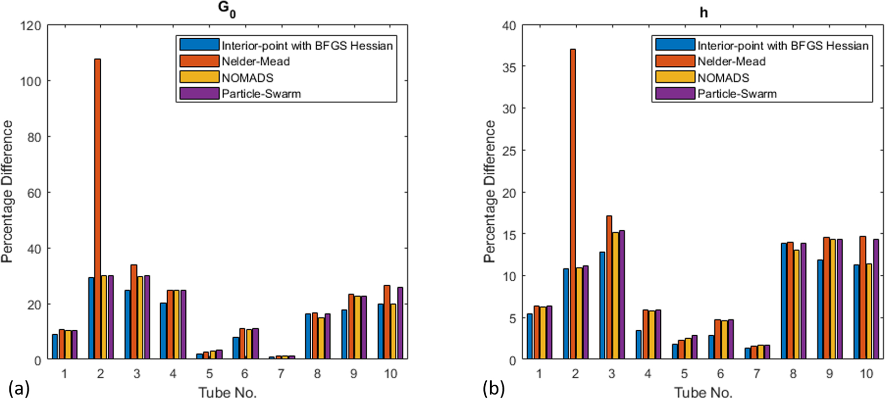
Error in the inverted shear-modulus parameter, G0 (a) and thicknesses, h (b).
Figure 11.
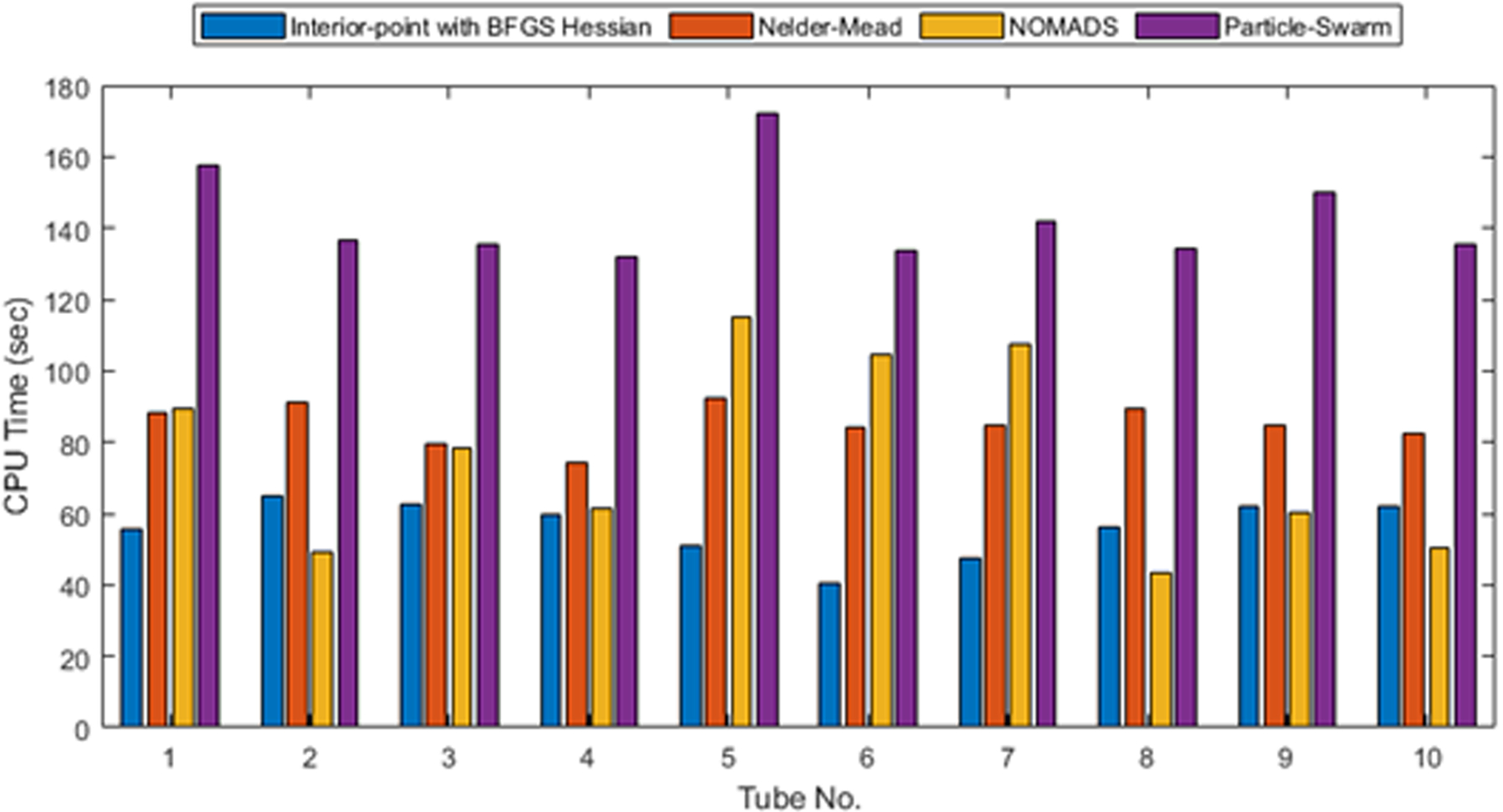
CPU time for combined inversion for modulus and thickness.
As we observe for tube 2, both inversion analyses (modulus as well as modulus-thickness inversion), the percent difference is quite high compared to the other tubes. This can be justified by looking at the measured dispersion curves for this tube as shown in Figure 12 (a). Recall that we apply the acoustic radiation force individually at six angular positions and repeat the acquisition ten times for each of the six angular positions. In the case of tube 2, we notice good correlation within each set of ten acquisitions, but low correlation across the six angular cases. This indicates the tube may not be homogeneous due to imperfect fabrication. On the other hand, tube 5, which has yielded lower error in the inversion analysis, has tight correlation across all acquisitions and angular cases as presented in Figure 12 (b). With respect to the significantly high error for tube 2 with the Nelder-Mead algorithm (inversion for both modulus and thickness), the solution seemed to have converged to a local minima far from the solution as the underlying optimization framework does not allow any constraints. This is a reason, in addition to computational cost, that we propose to use BFGS approach as the method of choice.
Figure 12.
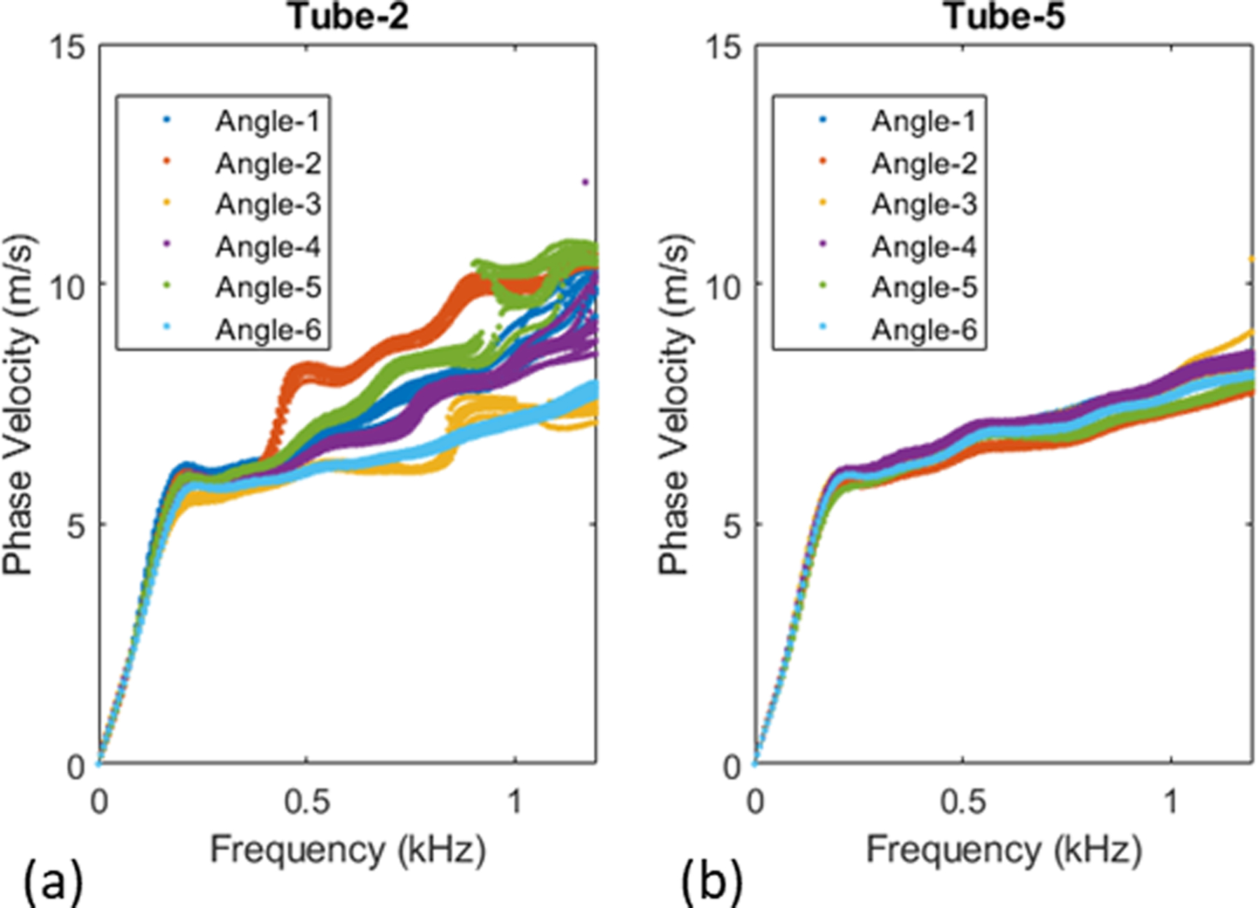
Measured dispersion curves for Tube-2 (a) and Tube-5 (b)
Effect of data processing:
Earlier in the paper, we illustrated that data processing details are critical to obtaining accurate dispersion curves. However, dispersion curves are only of intermediate interest, with the final objective being the modulus estimation. The natural question then is, what if the inversion is performed without the data processing refinements? We performed this exercise and observed that standard data processing resulted in an average modulus error of 22.4% compared to a significantly reduced error of 5% when the data processing refinements are employed.
Effect of multimodal inversion:
Another important question that may arise is: how important is it to match with different simulated curves for the two frequency ranges (multi-modal inversion)? What if the inversion is performed by matching with a single, fundamental dispersion curve for both frequency ranges (single-mode inversion)? For example, when applied to tube 1, it turns out that single-mode inversion (with the first mode, n = 1) results in higher errors in the estimated modulus (10.6%) compared to that from multi-modal inversion (0.6%), confirming the benefit of multimodal inversion.
The proposed study is only a step towards estimation of arterial stiffness using ARF excitation. The issues that require attention before applying it to in vivo data from human arteries include: (a) automatic determination of signal processing parameters (they are currently determined manually); (b) estimating the frequency dependence directly from ARF measurements instead of using the information from Rheospectris measurements; (c) validation studies for differing thicknesses (we validated the model with single thickness of 1 mm as dictated by the mold and it would be useful to validate for other thicknesses); (d) optimizing the experimental setup including the number of acquisitions (the number of acquisitions and orientations are chosen arbitrarily in this paper, erring on the conservative side), (e) validation using ex vivo data, e.g. using porcine aortas; and (f) examining the effect of surrounding tissues as well as physiological motion. Further research is underway in several of these directions and will be reported in the future.
Conclusions
This paper presents a new shear wave elastography (SWE) approach to estimate the arterial stiffness from acoustic radiation force measurements. The methodology is built on various refinements in different steps of SWE: (a) signal processing refinements through simple windowing informed by physical understanding, (b) efficient forward model for incompressible viscoelastic tubes, and (c) inversion by matching the measured dispersion curve with not one, but two separate dispersion curves (multimodal inversion). Through validation studies using extensive ARF experimental data, we observed that the proposed inversion approach results in high accuracy in estimating the shear modulus (less than 4% in 70% of the cases). We also observed that not using signal processing improvements or multimodal inversion degrades the accuracy of the modulus estimates. Finally, owing to the computational efficiency of the underlying forward model, the inversion procedure is highly efficient, taking less than 20 seconds on a regular computer.
In addition to inverting for just shear modulus, we also explored the possibility of simultaneous inversion of both shear modulus and wall thickness. The resulting accuracy is not as good as the accuracy of inverting for just shear modulus. Given this, at this time, we suggest measuring the wall thickness and then estimating the modulus from the proposed inversion framework. For in vivo settings, the thickness measured from ultrasound images may not be accurate, but will be close to the actual value, with some level of known error variance based on the transducer. Thus, the measured thickness can be used as prior information in a simultaneous probabilistic inversion for shear modulus and thickness. On the other hand, the radius, which is not as small as the thickness, can reliably be measured through ultrasound. Moreover, the dispersion curves are not as sensitive to radius perturbations as to thickness perturbations (Astaneh et al 2017). To address imperfect thickness measurements, fortunately, probabilistic inversion is feasible due to the efficiency of the forward model; this is the subject of ongoing research. In the current work, we fix the time/frequency dependency of the modulus and estimated the overall magnitude of the modulus. In reality, the complex viscoelastic modulus (both the amplitude and time dependency) needs to be estimated, which is also the subject of ongoing research. Finally, our study assumes isotropic elasticity, which is valid for phantom experiments. For real arteries, further beneficial enhancements would include: tissue anisotropy (Li et al 2017b, Shcherbakova et al 2017) and non-prismatic geometry (Karageorgos et al 2020, Wang and Lee 2020); these are subjects of future research.
Acknowledgements
The work is partially funded by National Science Foundation grant CMMI-1635291, and by National Institute of Health grant 5R01 HL145268. The content is solely the responsibility of authors and does not necessarily represent the official views of the National Science Foundation or the National Heart, Lung, and Blood Institute or the National Institutes of Health.
References
- Anon NOMAD - A blackbox optimization software Online: https://www.gerad.ca/nomad/
- Astaneh AV, Urban MW, Aquino W, Greenleaf JF and Guddati MN 2017. Arterial waveguide model for shear wave elastography: implementation and in vitro validation Phys. Med. Biol 62 5473–94 [DOI] [PubMed] [Google Scholar]
- Bernal M, Nenadic I, Urban MW and Greenleaf JF 2011. Material property estimation for tubes and arteries using ultrasound radiation force and analysis of propagating modes J. Acoust. Soc. Am 129 1344–54 [DOI] [PMC free article] [PubMed] [Google Scholar]
- Chirinos JA, Segers P, Hughes T and Townsend R 2019. Large-Artery Stiffness in Health and Disease: JACC State-of-the-Art Review J. Am. Coll. Cardiol 74 1237–63 [DOI] [PMC free article] [PubMed] [Google Scholar]
- Couade M, Pernot M, Prada C, Messas E, Emmerich J, Bruneval P, Criton A, Fink M and Tanter M 2010. Quantitative Assessment of Arterial Wall Biomechanical Properties Using Shear Wave Imaging Ultrasound Med. Biol 36 1662–76 [DOI] [PubMed] [Google Scholar]
- Currie J and Wilson DI 2012. Opti: Lowering the Barrier Between Open Source Optimizers and the Industrial MATLAB User ed Sahinidis N and Pinto J (Savannah, Georgia, USA: Foundations of Computer-Aided Process Operations; ) [Google Scholar]
- Datta S DK, Bratton RL, Chakraborty T and Shah AH 1988. Wave propagation in laminated composite plates J. Acoust. Soc. Am 83 2020–6 [Google Scholar]
- Dutta P, Urban MW, Le Maître OP, Greenleaf JF and Aquino W 2015. Simultaneous identification of elastic properties, thickness, and diameter of arteries excited with ultrasound radiation force Phys. Med. Biol 60 5279–96 [DOI] [PMC free article] [PubMed] [Google Scholar]
- Flamini V, Creane AP, Kerskens CM and Lally C 2015. Imaging and finite element analysis: A methodology for non-invasive characterization of aortic tissue Med. Eng. Phys 37 48–54 [DOI] [PubMed] [Google Scholar]
- Gazis DC 1959aThree-Dimensional Investigation of the Propagation of Waves in Hollow Circular Cylinders. I. Analytical Foundation J. Acoust. Soc. Am 31568–73 [Google Scholar]
- Gazis DC 1959bThree-dimensional investigation of the propagation of waves in hollow circular cylinders. ii. numerical results J. Acoust. Soc. Am 31573–8 [Google Scholar]
- Hadj Henni A, Schmitt C, Tremblay MÉ, Hamdine M, Heuzey MC, Carreau P and Cloutier G 2011. Hyper-frequency viscoelastic spectroscopy of biomaterials J. Mech. Behav. Biomed. Mater 4 1115–22 [DOI] [PubMed] [Google Scholar]
- Hughes TJR 2000The Finite Element Method: Linear Static and Dynamic Finite Element Analysis (Dover Civil and Mechanical Engineering) (Dover Publications; ) [Google Scholar]
- Jang JK, Kondo K, Namita T, Yamakawa M and Shiina T 2015. Comparison of techniques for estimating shear-wave velocity in arterial wall using shear-wave elastography - FEM and phantom study 2015 IEEE International Ultrasonics Symposium, IUS 2015 (Institute of Electrical and Electronics Engineers Inc.) [Google Scholar]
- Karageorgos GM, Apostolakis IZ, Nauleau P, Gatti V, Weber R, Connolly ES, Miller EC and Konofagou EE 2020. Arterial wall mechanical inhomogeneity detection and atherosclerotic plaque characterization using high frame rate pulse wave imaging in carotid artery disease patients in vivo Phys. Med. Biol 65 [DOI] [PMC free article] [PubMed] [Google Scholar]
- Kasai C, Namekawa K, Koyano A and Omoto R 1985. Real-Time Two-Dimensional Blood Flow Imaging Using an Autocorrelation Technique IEEE Trans. SONICS Ultrason 32 [Google Scholar]
- Kausel E and Peek R 1982. DYNAMIC LOADS IN THE INTERIOR OF A LAYERED STRATUM: AN EXPLICIT SOLUTION vol 72 [Google Scholar]
- Kennedy J and Eberhart R 1995. Particle swarm optimization Proceedings of ICNN’95 - International Conference on Neural Networks vol 4 (IEEE; ) pp 1942–8 [Google Scholar]
- Kijanka P, Qiang B, Song P, Amador Carrascal C, Chen S and Urban MW 2018. Robust Phase Velocity Dispersion Estimation of Viscoelastic Materials Used for Medical Applications Based on the Multiple Signal Classification Method IEEE Trans. Ultrason. Ferroelectr. Freq. Control 65 423–39 [DOI] [PMC free article] [PubMed] [Google Scholar]
- Kijanka P and Urban MW 2021a. Dispersion curve calculation in viscoelastic tissue-mimicking materials using non-parametric, parametric, and high-resolution methods Ultrasonics 109 106257. [DOI] [PMC free article] [PubMed] [Google Scholar]
- Kijanka P and Urban MW 2021b. Phase Velocity Estimation with Expanded Bandwidth in Viscoelastic Phantoms and Tissues IEEE Trans. Med. Imaging [DOI] [PMC free article] [PubMed] [Google Scholar]
- Kullo IJ and Malik AR 2007. Arterial Ultrasonography and Tonometry as Adjuncts to Cardiovascular Risk Stratification J. Am. Coll. Cardiol 49 1413–26 [DOI] [PubMed] [Google Scholar]
- Lagarias JC, Reeds JA, Wright MH, Wright PE and Optim SJ 1998. CONVERGENCE PROPERTIES OF THE NELDER-MEAD SIMPLEX METHOD IN LOW DIMENSIONS SIAM J. Optim 9 112–47 [Google Scholar]
- Laurent S, Cockcroft J, Van Bortel L, Boutouyrie P, Giannattasio C, Hayoz D, Pannier B, Vlachopoulos C, Wilkinson I and Struijker-Boudier H 2006. Expert consensus document on arterial stiffness: Methodological issues and clinical applications Eur. Heart J 27 2588–605 [DOI] [PubMed] [Google Scholar]
- Li GY, He Q, Jia L, He P, Luo J and Cao Y 2017a. An Inverse Method to Determine Arterial Stiffness with Guided Axial Waves Ultrasound Med. Biol 43 505–16 [DOI] [PubMed] [Google Scholar]
- Li GY, He Q, Mangan R, Xu G, Mo C, Luo J, Destrade M and Cao Y 2017b. Guided waves in pre-stressed hyperelastic plates and tubes: Application to the ultrasound elastography of thin-walled soft materials J. Mech. Phys. Solids 102 67–79 [Google Scholar]
- Lin SM, Wang WR, Lee SY, Chen CW, Hsiao YC and Teng MJ 2015. Wave modes of a pre-stressed thick tube conveying blood on the viscoelastic foundation Appl. Math. Model 39 466–82 [Google Scholar]
- Luo J, Fujikura K, Tyrie LS, Tilson MD and Konofagou EE 2009. Pulse wave imaging of normal and aneurysmal abdominal aortas in vivo IEEE Trans. Med. Imaging 28 477–86 [DOI] [PubMed] [Google Scholar]
- Luo J, Li RX and Konofagou EE 2012. Pulse wave imaging of the human carotid artery: An in vivo feasibility study IEEE Trans. Ultrason. Ferroelectr. Freq. Control 59 174–81 [DOI] [PMC free article] [PubMed] [Google Scholar]
- Maksuti E, Bini F, Fiorentini S, Blasi G, Urban MW, Marinozzi F and Larsson M 2017. Influence of wall thickness and diameter on arterial shear wave elastography: a phantom and finite element study Phys. Med. Biol 62 2694–718 [DOI] [PubMed] [Google Scholar]
- Maksuti E, Widman E, Larsson D, Urban MW, Larsson M and Bjällmark A 2016. Arterial Stiffness Estimation by Shear Wave Elastography: Validation in Phantoms with Mechanical Testing Ultrasound Med. Biol 42 308–21 [DOI] [PubMed] [Google Scholar]
- Marais L, Pernot M, Khettab H, Tanter M, Messas E, Zidi M, Laurent S and Boutouyrie P 2019. Arterial Stiffness Assessment by Shear Wave Elastography and Ultrafast Pulse Wave Imaging: Comparison with Reference Techniques in Normotensives and Hypertensives Ultrasound Med. Biol 45 758–72 [DOI] [PubMed] [Google Scholar]
- McGarry M, Li R, Apostolakis I, Nauleau P and Konofagou EE 2016. An inverse approach to determining spatially varying arterial compliance using ultrasound imaging Phys. Med. Biol 61 5486–507 [DOI] [PMC free article] [PubMed] [Google Scholar]
- Nelson RB, Dong SB and Kalra RD 1971. Vibrations and waves in laminated orthotropic circular cylinders J. Sound Vib 18 429–44 [Google Scholar]
- Nguyen TM, Couade M, Bercoff J and Tanter M 2011. Assessment of viscous and elastic properties of sub-wavelength layered soft tissues using shear wave spectroscopy: Theoretical framework and in vitro experimental validation IEEE Trans. Ultrason. Ferroelectr. Freq. Control 58 2305–15 [DOI] [PubMed] [Google Scholar]
- Palombo C and Kozakova M 2016. Arterial stiffness, atherosclerosis and cardiovascular risk: Pathophysiologic mechanisms and emerging clinical indications Vascul. Pharmacol 77 1–7 [DOI] [PubMed] [Google Scholar]
- Parameswaran PK, Dai D, Ding YH, Urban MW, Manlove L, Sathish V, Cebral JR, Kallmes DF and Kadirvel R 2019. Downstream vascular changes after flow-diverting device deployment in a rabbit model J. Neurointerv. Surg 11 523–7 [DOI] [PMC free article] [PubMed] [Google Scholar]
- Pruijssen JT, de Korte CL, Voss I and Hansen HHG 2020. Vascular Shear Wave Elastography in Atherosclerotic Arteries: A Systematic Review Ultrasound Med. Biol 46 2145–63 [DOI] [PubMed] [Google Scholar]
- Rose JL 2014Ultrasonic Guided Waves in Solid Media (Cambridge University Press; ) [Google Scholar]
- Roy T and Guddati MN 2021. Shear wave dispersion analysis of incompressible waveguides J. Acoust. Soc. Am 149 972–82 [DOI] [PMC free article] [PubMed] [Google Scholar]
- Saltelli A, Ratto M, Andres T, Campolongo F, Cariboni J, Gatelli D, Saisana M and Tarantola S 2007. Global Sensitivity Analysis. The Primer (Chichester, UK: John Wiley & Sons, Ltd; ) [Google Scholar]
- Savadatti S and Guddati MN 2010. A finite element alternative to infinite elements Comput. Methods Appl. Mech. Eng 199 2204–23 [Google Scholar]
- Segers P, Rietzschel ER and Chirinos JA 2020. How to Measure Arterial Stiffness in Humans Arterioscler. Thromb. Vasc. Biol 1034–43 [DOI] [PMC free article] [PubMed] [Google Scholar]
- Shcherbakova DA, Debusschere N, Caenen A, Iannaccone F, Pernot M, Swillens A and Segers P 2017. A finite element model to study the effect of tissue anisotropy on ex vivo arterial shear wave elastography measurements Phys. Med. Biol 62 5245–75 [DOI] [PubMed] [Google Scholar]
- Smith RC 2013Uncertainty quantification : theory, implementation, and applications (SIAM in the Computational Science and Engineering Series; ) [Google Scholar]
- Sun Z 2015Aging, arterial stiffness, and hypertension Hypertension 65252–6 [DOI] [PMC free article] [PubMed] [Google Scholar]
- Tran TNHT, Nguyen KCT, Sacchi MD and Le LH 2014. Imaging Ultrasonic Dispersive Guided Wave Energy in Long Bones Using Linear Radon Transform Ultrasound Med. Biol 40 2715–27 [DOI] [PubMed] [Google Scholar]
- Vappou J, Luo J and Konofagou EE 2010. Pulse Wave Imaging for Noninvasive and Quantitative Measurement of Arterial Stiffness In Vivo Am. J. Hypertens 23 393–8 [DOI] [PMC free article] [PubMed] [Google Scholar]
- Vaziri Astaneh A and Guddati M 2017. Dispersion analysis software for immersed and embedded waveguides Online: http://wavedisp.com
- Vlachopoulos C, Aznaouridis K and Stefanadis C 2010. Prediction of Cardiovascular Events and All-Cause Mortality With Arterial Stiffness. A Systematic Review and Meta-Analysis J. Am. Coll. Cardiol 55 1318–27 [DOI] [PubMed] [Google Scholar]
- Waltz RA, Morales JL, Nocedal J and Orban D 2006. An interior algorithm for nonlinear optimization that combines line search and trust region steps Math. Program., Ser. A 107 391–408 [Google Scholar]
- Wang Y and Lee W-N 2020. Non-invasive Estimation of Localized Dynamic Luminal Pressure Change by Ultrasound Elastography in Arteries with Normal and Abnormal Geometries IEEE Trans. Biomed. Eng 9294 1–1 [DOI] [PubMed] [Google Scholar]
- Widman E, Maksuti E, Amador C, Urban MW, Caidahl K and Larsson M 2016. Shear Wave Elastography Quantifies Stiffness in Ex Vivo Porcine Artery with Stiffened Arterial Region Ultrasound Med. Biol 42 2423–35 [DOI] [PubMed] [Google Scholar]
- Widman E, Maksuti E, Larsson D, Urban MW, Bjällmark A and Larsson M 2015. Shear wave elastography plaque characterization with mechanical testing validation: A phantom study Phys. Med. Biol 60 3151–74 [DOI] [PubMed] [Google Scholar]
- Zhang X, Kinnick RR, Fatemi M and Greenleaf JF 2005. Noninvasive method for estimation of complex elastic modulus of arterial vessels IEEE Trans. Ultrason. Ferroelectr. Freq. Control 52 642–51 [DOI] [PubMed] [Google Scholar]


