Variance and limiting distribution of coalescence times in a diploid model of a consanguineous population

Abstract

Recent modeling studies interested in runs of homozygosity (ROH) and identity by descent (IBD) have sought to connect these properties of genomic sharing to pairwise coalescence times. Here, we examine a variety of features of pairwise coalescence times in models that consider consanguinity. In particular, we extend a recent diploid analysis of mean coalescence times for lineage pairs within and between individuals in a consanguineous population to derive the variance of coalescence times, studying its dependence on the frequency of consanguinity and the kinship coefficient of consanguineous relationships. We also introduce a separation-of-time-scales approach that treats consanguinity models analogously to mathematically similar phenomena such as partial selfing, using this approach to obtain coalescence-time distributions. This approach shows that the consanguinity model behaves similarly to a standard coalescent, scaling population size by a factor 1 − 3c, where c represents the kinship coefficient of a randomly chosen mating pair. It provides the explanation for an earlier result describing mean coalescence time in the consanguinity model in terms of c. The results extend the potential to make predictions about ROH and IBD in relation to demographic parameters of diploid populations.

1. Introduction

Previously (Severson et al., 2019), we devised a coalescent model of a consanguineous diploid population in order to jointly study runs of homozygosity (ROH) and identity-by-descent (IBD) sharing. We used the fact that the time to the most recent common ancestor at a single-base-pair site for a pair of genomes is inversely related to the length of the shared segment around the site (PALAMARA et al., 2012; CARMI et al., 2014). To distinguish within-individual from between-individual coalescence times, which influence levels of within-individual ROH and between-individual IBD sharing, we modeled a diploid biparental population.

We developed our model by extending the diploid sib mating model of CAMPBELL (2015) to allow nth cousin mating and a superposition of multiple degrees of cousin mating. To derive mean pairwise coalescence times in our models, we performed a first-step analysis of a Markov chain to condition on the state of two alleles in prior generations. We found that owing to the possibility of extremely recent coalescence from consanguinity, the effect of consanguinity reduced mean pairwise coalescence times within an individual as well as between separate individuals. The reduction of the mean coalescence time was proportional to the kinship coefficient of a randomly chosen mating pair, with a greater reduction for two alleles within an individual versus between individuals.

Although mean coalescence times are useful for summarizing the effect of consanguinity under the model, and they reveal that both within- and between-individual coalescence times depend on population size and consanguinity, the mean describes only one aspect of the distribution. Distributions of pairwise coalescence times within and between individuals are needed to more fully understand the effect of consanguinity on the length of shared segments within and between individuals (PALAMARA et al., 2012; CARMI et al., 2014).

Coalescent-based population-genetic models typically approximate a two-sex diploid population of size N individuals with a haploid population of size 2N. In a diploid model, two alleles can be either within an individual or in separate individuals, whereas in a haploid model, all alleles are exchangeable. Despite this distinction, with a sufficiently large population size and equal numbers of males and females, the ancestral process of a diploid population converges to that of a haploid population of twice the size, supporting the approximation (WAKELEY, 2009, Chapter 6.1). Intuitively, the convergence occurs when the probability of rapid coalescence of the two alleles in a diploid individual is negligible.

A variety of techniques have been used to analyze coalescent models, in which, like in consanguinity models, rapid coalescence cannot be ignored. WAKELEY et al. (2012) examined the effect of a fixed diploid population pedigree on coalescence times, finding that the probability of recent coalescence events is slightly increased compared to a corresponding haploid model. Models of partial selfing (NORDBORG and DONNELLY, 1997; MÖHLE, 1998b) have examined the effect of a selfing rate that gives the probability of immediate coalescence of pairs of alleles in a diploid individual. This work has used the separation-of-time-scales approach (MÖHLE, 1998b), which describes the concurrent effect of a “fast” coalescent process (coalescence of two alleles from an individual due to selfing) and a “slow” process (coalescence of pairs of alleles in the population at large).

Here, we continue our earlier work to further investigate the distributions of coalescence times for pairs of alleles within and between individuals in a diploid coalescent model with consanguinity. First, we derive the variance of coalescence times under sib mating and extend the calculation to the superposition case. Next, we use a separation-of-time-scales approach to derive the distributions of pairwise coalescence times within and between individuals in the limit of large population size. We compare the mean and variance of these limiting distributions to the exact solutions. We also compare the full limiting distribution to numerical solutions in the sib mating case, and also to the results of simulations from the exact Markov chains. We find that the limiting distributions closely approximate the exact distributions.

2. Model

We extend the model of SEVERSON et al. (2019), which itself extended the model of CAMPBELL (2015). The model considers a constant-sized diploid population with discrete generations. Each generation has N ≥ 2 monogamous mating pairs, 2N diploid individuals, and 4N alleles at each locus. A constant fraction of the mating pairs are consanguineous unions, and the other pairs are non-consanguineous. The fraction of mating pairs each generation that are related as nth cousins is denoted c_n (Figure 1A).

Figure 1:

Diploid model of sib mating. (A) In each generation, a fraction c₀ = 0.4 of N = 5 mating pairs are sib mating pairs. (B) Sib mating pairs are each assigned a parental pair from the previous generation. (C) Non-consanguineous pairs are each assigned two distinct parental pairs, representing the two sets of parents for the two individuals in the non-consanguineous pair.

To illustrate the model, we consider a simple case, a population with sib mating, viewing sibs as 0th cousins. Backward in time, the $c_{0}N$ sib mating pairs—each of whose two individuals necessarily share a single set of parents—each randomly choose one parental mating pair from the previous generation (Figure 1B). Next, the (1−c₀)N random-mating pairs each randomly choose two distinct parental mating pairs (Figure 1C). Note that two individuals in a random-mating pair cannot share the same parental mating pair, so that chance sib mating is forbidden. Because parental mating pairs are chosen at random, two individuals in separate mating pairs will be siblings with probability $\frac{1}{N}$.

In this model, two alleles at a locus can be in three possible states, denoted 1, 2, and 3. State 1 corresponds to two alleles within an individual, state 2 is for two alleles in two distinct individuals in a mating pair, and state 3 is two alleles in two distinct individuals in separate mating pairs. We use the random variables T, U, and V to denote the coalescence times for two alleles in states 1, 2, and 3, respectively.

3. Variance of coalescence times

3.1. Sib mating

We begin with a sib mating population. In each generation, a constant fraction c₀ of the N mating pairs are siblings, and chance sib mating is forbidden. Previously, we derived the means for T, U, and V as (SEVERSON et al., 2019, eqs. 4–6)

$$\mathbb{E}[T]=4N\left(1-c_0\right)+6$$ (1)

$$\mathbb{E}[U]=4N\left(1-c_0\right)+5$$ (2)

$$\mathbb{E}[V]=4N\left(1-\frac{3}{4}{c}_0\right)+4.$$ (3)

Here we derive the variances for T, U, and V. First, two alleles that are within an individual (state 1) are always in two individuals in a mating pair in the previous generation (state 2), so $T=U+1$ and

$$\text{Var}[T]=\text{Var}[U].$$ (4)

Next we derive Var[U] using the law of total variance. For convenience, we define the random variable Z to be the state of two alleles in the previous generation. We add state 0 to represent coalescence, so Z takes values from {0,1,2,3}. Applying the law of total variance and conditioning on Z, $\text{Var}[U]={\mathbb{E}}_Z[\text{Var}[U\mid Z]]+{\text{Var}}_Z[\mathbb{E}[U\mid Z]]$.

Beginning with ${\mathbb{E}}_Z[\text{Var}[U\mid Z]]$, if two alleles are in a mating pair (state 2), then the previous generation has four possible states, encoded in values of Z. First, with probability c₀, the mating pair is a sib mating pair. In this case, with probability $\frac{1}{4}$, the alleles coalesce in the previous generation (Z = 0) and the alleles have coalescence time 1. Similarly, if the mating pair is consanguineous (i.e., sibs), then with probability $\frac{1}{4}$, the alleles were inherited from the same individual (Z = 1), and they have coalescence time T + 1. Lastly if the mating pair is a sib mating pair, then with probability $\frac{1}{2}$, the two alleles were inherited from separate parents in the previous generation (Z = 2), and the two alleles have coalescence time U + 1. With probability 1 − c₀, the two alleles are in a random-mating pair, in the previous generation they were in two individuals in separate mating pairs (Z = 3), and they have coalescence time V + 1. Combining these cases gives

$${\mathbb{E}}_Z[\text{Var}[U\mid Z]]=\frac{c_0}{4}\text{Var}[1]+\frac{c_0}{4}\text{Var}[T+1]+\frac{c_0}{2}\text{Var}[U+1]+\left(1-c_0\right)\text{Var}[V+1].$$ (5)

For the next term, ${\text{Var}}_Z[\mathbb{E}[U\mid Z]]$, we rewrite it using the definition of variance, ${\text{Var}}_Z[\mathbb{E}[U\mid Z]]={\mathbb{E}}_Z\left[\mathbb{E}{[U\mid Z]}^2\right]-{\left({\mathbb{E}}_Z[\mathbb{E}[U\mid Z]]\right)}^2={\mathbb{E}}_Z\left[\mathbb{E}{[U]}^2\right]-\mathbb{E}{[U]}^2$. Because $\mathbb{E}{[U]}^2$ is known (eq. 2), we only need ${\mathbb{E}}_Z\left[\mathbb{E}{[U\mid Z]}^2\right]$, which we derive by again conditioning on Z. With probability c₀/4, the alleles coalesce in 1 generation (Z = 0). With probability c₀/4, the alleles were inherited from the same individual (Z = 1), and $\mathbb{E}{[U\mid Z=1]}^2=\mathbb{E}{[T+1]}^2$. With probability c₀/2, the alleles were inherited from separate individuals in the same mating pair (Z = 2), and $\mathbb{E}{[U\mid Z=2]}^2=\mathbb{E}{[U+1]}^2$. Lastly, with probability 1 − c₀, the alleles are in a non-consanguineous mating pair and they were inherited from two individuals in separate mating pairs (Z = 3), giving $\mathbb{E}{[U\mid Z=3]}^2=\mathbb{E}{[V+1]}^2$. Combining these cases gives

$${\mathbb{E}}_Z\left[\mathbb{E}{[U\mid Z]}^2\right]=\frac{c_0}{4}{(1)}^2+\frac{c_0}{4}{(\mathbb{E}[T]+1)}^2+\frac{c_0}{2}{(\mathbb{E}[U]+1)}^2+\left(1-c_0\right){(\mathbb{E}[V]+1)}^2.$$

Subtracting $\mathbb{E}{[U]}^2$, we have

$${\text{Var}}_Z[\mathbb{E}[U\mid Z]]=\frac{c_0}{4}{(1)}^2+\frac{c_0}{4}{(\mathbb{E}[T]+1)}^2+\frac{c_0}{2}{(\mathbb{E}[U]+1)}^2+\left(1-c_0\right){(\mathbb{E}[V]+1)}^2-\mathbb{E}{[U]}^2.$$ (6)

Summing eqs. 5 and 6, applying eq. 4 and $\mathbb{E}[T]=\mathbb{E}[U]+1$, and simplifying gives

$$\text{Var}[U]=\left(\frac{4-4c_0}{4-3c_0}\right)\left[\text{Var}[V]+{(\mathbb{E}[V]+1)}^2\right]-\mathbb{E}{[U]}^2+\frac{8c_0}{4-3c_0}\mathbb{E}[U]+\frac{7c_0}{4-3c_0}.$$ (7)

Next, for Var[V], we again use the law of total variance and condition on Z. For the first term ${\mathbb{E}}_Z[\text{Var}[V\mid Z]]$, recall that if two alleles are in two separate mating pairs, then because parents are chosen randomly with replacement, the two individuals are siblings with probability $\frac{1}{N}$. Then the probability that the two alleles are in two individuals who are siblings and that those alleles coalesce in the previous generation (Z = 0) is $\frac{1}{4N}$. Similarly, the probability that the siblings inherit distinct alleles from the same parent (Z = 1) is $\frac{1}{4N}$, giving a coalescence time of T + 1. If the alleles are inherited from separate parents (Z = 2), an event with probability $\frac{1}{2N}$, then the coalescence time is U + 1. Lastly, with probability $1-\frac{1}{N}$, the individuals are not siblings, so the alleles were inherited from separate individuals in separate mating pairs (Z = 3), giving coalescence time V + 1. These four cases give

$${\mathbb{E}}_Z[\text{Var}[V\mid Z]]=\frac{1}{4N}\text{Var}[1]+\frac{1}{4N}\text{Var}[T+1]+\frac{1}{2N}\text{Var}[U+1]+\left(1-\frac{1}{N}\right)\text{Var}[V+1].$$ (8)

For ${\text{Var}}_Z[\mathbb{E}[V\mid Z]]={\mathbb{E}}_Z\left[\mathbb{E}{[V\mid Z]}^2\right]-{\left({\mathbb{E}}_Z[\mathbb{E}[V\mid Z]]\right)}^2$, we have ${\mathbb{E}}_Z[\mathbb{E}[V\mid Z]]=\mathbb{E}[V]$ as before. For ${\mathbb{E}}_Z\left[\mathbb{E}{[V\mid Z]}^2\right]$, if two alleles are in two individuals in separate mating pairs, then with probability $\frac{1}{N}$, the individuals are siblings. If Z = 0, then the alleles coalesce in the previous generation with probability $\frac{1}{4N}$. If Z = 1, then the two alleles were inherited from the same individual in the previous generation. This event occurs with probability $\frac{1}{4N}$, and $\mathbb{E}{[V\mid Z=1]}^2=\mathbb{E}{[T+1]}^2$. With probability $\frac{1}{2N}$, Z = 2, and the alleles were inherited from two individuals in a mating pair, giving $\mathbb{E}{[V\mid Z=2]}^2=\mathbb{E}{[U+1]}^2$. Lastly, with probability $1-\frac{1}{N}$, the two individuals are not siblings, so the alleles were inherited from two individuals in separate mating pairs (Z = 3), and $\mathbb{E}{[V\mid Z=3]}^2=\mathbb{E}{[V+1]}^2$. Combining cases and subtracting $\mathbb{E}$[V]² gives the second term

$${\text{Var}}_Z[\mathbb{E}[V\mid Z]]=\frac{1}{4N}{(1)}^2+\frac{1}{4N}{(\mathbb{E}[T]+1)}^2+\frac{1}{2N}{(\mathbb{E}[U]+1)}^2+\left(1-\frac{1}{N}\right){(\mathbb{E}[V]+1)}^2-\mathbb{E}{[V]}^2.$$ (9)

Summing eqs. 8 and 9, applying eq. 4 and $\mathbb{E}[T]=\mathbb{E}[U]+1$, and simplifying gives the form

$$\text{Var}[V]=\frac{3}{4}\left[\text{Var}[U]+\mathbb{E}{[U]}^2+1\right]+2\mathbb{E}[U]-\mathbb{E}{[V]}^2+2(N-1)\mathbb{E}[V]+N.$$ (10)

Eqs. 4, 7, and 10 form a linear system in Var[T], Var[U], and Var[V], which we solve, applying eqs. 1–3:

$$\text{Var}[T]=\text{Var}[U]=16N^2\left(1-c_0\right)\left(1-\frac{1}{2}{c}_0\right)+28N\left(1-c_0\right)+22$$ (11)

$$\text{Var}[V]=16N^2{\left(1-\frac{3}{4}{c}_0\right)}^2+28N\left(1-\frac{29}{28}{c}_0\right)+22.$$ (12)

Eqs. 11 and 12 give the desired variances. We can immediately make a number of observations.

First, considering all possible consanguinity levels c₀, both eqs. 11 and 12 are maximized when c₀ = 0, and they decrease with increasing c₀. Thus, consanguinity decreases variance for all three coalescence times.

Next, the difference Var[V] − Var[T] equals $N^2{c}_0^2-N{c}_0$, which is positive for $c_0>\frac{1}{N}$, so that $\text{Var}[V]>\text{Var}[T]$. Thus, with a nontrivial consanguinity level, the variance of the coalescence time for two alleles in separate mating pairs exceeds that for two alleles in the same individual.

Third, taking N → ∞, eqs. 11 and 12 give

$$\frac{\text{Var}[T]}{16N^2}=\frac{\text{Var}[U]}{16N^2}=\left(1-c_0\right)\left(1-\frac{1}{2}{c}_0\right)$$ (13)

$$\frac{\text{Var}[V]}{16N^2}={\left(1-\frac{3}{4}{c}_0\right)}^2.$$ (14)

Thus, for large N, the variances are dominated by the product of 16N², the variance of coalescence time for a haploid population of size 4N, and a reduction factor $\left(1-c_0\right)\left(1-\frac{1}{2}{c}_0\right)$ in eq. 11 and ${\left(1-\frac{3}{4}{c}_0\right)}^2$ in eq. 12.

In the standard coalescent model of a non-consanguineous diploid population of size 2N individuals, the mean pairwise coalescence time is exponentially distributed with mean 4N. We thus examine the extent to which the pairwise coalescence time in our diploid consanguinity model follows an exponential distribution. Using eqs. 3 and 12, note that in the limit of large N, $\text{Var}[V]/\mathbb{E}{[V]}^2\to 1$. Recall that an exponentially distributed random variable with mean λ has variance λ², so the variance is the square of the mean. Although this relationship is not unique to the exponential distribution, the fact that $\text{Var}[V]/\mathbb{E}{[V]}^2\to 1$ is consistent with V being exponentially distributed in the limit as N → ∞. On the other hand, $\text{Var}[T]/\mathbb{E}{[T]}^2\to \left(2-c_0\right)/\left(2-2c_0\right)$, so T is not exponentially distributed in the N → ∞ limit for c₀ > 0.

Eqs. 11 and 12 normalized by 16N² are plotted in Figure 2 as a function of the number of mating pairs N and fraction of sib mating pairs c₀. As population size increases, the normalized variances quickly approach the reduction factors, $\left(1-c_0\right)\left(1-\frac{1}{2}{c}_0\right)$ in eq. 11 and ${\left(1-\frac{3}{4}{c}_0\right)}^2$ in eq. 12.

Figure 2:

Normalized variance of pairwise coalescence times as a function of the number of mating pairs N and the fraction of sib mating pairs c₀. (A) Var[T]/(16N²), eq. 11. (B) Var[V]/(16N²), eq. 12. Dashed lines represent limiting reduction factors due to consanguinity as $N\to \infty ,\left(1-c_0\right)\left(1-\frac{1}{2}{c}_0\right)$ in (A) (eq. 13) and ${\left(1-\frac{3}{4}{c}_0\right)}^2$ in (B) (eq. 14).

3.2. Superposition of multiple mating levels

In this section, we generalize the variance under sib mating to a superposition of multiple levels of cousin mating. Under the superposition, ith cousin mating is permitted for all i from 0 to n, where n is the degree of the most distant permissible cousin relationship. The case of i = 0 corresponds to sib mating. For each i, let c_i be the fraction of ith cousin mating pairs in each generation. For each i ≤ n, chance ith cousin mating is prohibited. We assume individuals in a consanguineous mating pair share only one line of descent—that is, for example, they cannot be both first and third cousins. This assumption is designed for a large population and a small value of the sum of consanguinity rates, ${\sum }_{i=0}^n{c}_i\ll 1$.

Under this model, we derived the means for T, U, and V as (SEVERSON et al., 2019, eqs. 17–19)

$$\mathbb{E}[T]=4N(1-4c)+4n(1-4c)+16d+6$$ (15)

$$\mathbb{E}[U]=4N(1-4c)+4n(1-4c)+16d+5$$ (16)

$$\mathbb{E}[V]=4N(1-3c)+3n(1-4c)+12d+4,$$ (17)

where c, the kinship coefficient for two individuals in a mating pair, is defined as

$$c=\sum _{i=0}^n\frac{c_i}{4^{i+1}},$$ (18)

and for convenience, we define d as

$$d=\sum _{i=0}^n\frac{i{c}_i}{4^{i+1}}.$$ (19)

First for Var[T], as before, two alleles present within an individual are in two individuals in a mating pair in the previous generation, so T = U + 1 and eq. 4 continues to hold.

To derive Var[U], we again use the law of total variance and condition on Z. Before, if two individuals in a mating pair were siblings, then the alleles could transition to one of four states in the previous generation. Under the superposition, there are instead 3(n + 1) + 1 possible transitions. For each i, $0\le i\le n$, if the two individuals in the mating pair are ith cousins, then i + 1 generations in the past, the two alleles are inherited from the shared ancestral mating pair with probability 1/4ⁱ. If the alleles are inherited from the shared ancestral mating pair, then i + 1 generations ago they can transition to states 0, 1, or 2, giving 3(n + 1) possible transitions when considering all i from 0 to n. If the two individuals in the mating pair are not related, then because chance nth cousin mating is forbidden, n + 1 generations ago the alleles are in state 3, accounting for the last of the 3(n + 1) + 1 transitions.

For the first term in the law of total variance, ${\mathbb{E}}_Z[\text{Var}[U\mid Z]]$, we consider ith cousin mating for each i. With probability $c_i/4^i$, the individuals are ith cousins and the two alleles were inherited from the shared ancestral mating pair i + 1 generations ago. If the alleles are inherited from this mating pair, then with probability $\frac{1}{4}$, they coalesce in time i + 1; with probability $\frac{1}{4}$, the alleles are inherited from the same individual in the mating pair, with coalescence time T + i + 1; and with probability $\frac{1}{2}$, the alleles are inherited from separate individuals in the shared ancestral mating pair and have coalescence time U + i + 1. If for all i, 0 ≤ i ≤ n, the two individuals are not ith cousins, or if they are ith cousins for some i but the alleles are not inherited from the shared ancestral mating pair, then they are in two individuals in separate mating pairs n + 1 generations ago; this event has probability $1-{\sum }_{i=0}^n{c}_i/4^i$, and the alleles have coalescence time $V+i+1$. Summing the probabilities of the cases for $0\le i\le n$,

$${\mathbb{E}}_Z[\text{Var}[U\mid Z]]=\sum _{i=0}^n\frac{c_i}{4^i}\left[\frac{\text{Var}[i+1]}{4}+\frac{\text{Var}[T+i+1]}{4}+\frac{\text{Var}[U+i+1]}{2}\right]+\left(1-\sum _{i=0}^n\frac{c_i}{4^i}\right)\text{Var}[V+n+1].$$ (20)

For the second term ${\text{Var}}_Z[\mathbb{E}[U\mid Z]]$, we derive ${\mathbb{E}}_Z\left[\mathbb{E}{[U\mid Z]}^2\right]$. Again if the two individuals in the mating pair are ith cousins, then with probability $c_i/4^i$, the alleles were inherited from the shared ancestral mating pair i + 1 generations ago. If the alleles were inherited from the ancestral mating pair, then there are three possible transitions: with probability $\frac{1}{4}$, they coalesce with time i+1; with probability $\frac{1}{4}$, they were inherited from the same individual, giving mean $\mathbb{E}{[T+i+1]}^2$; with probability $\frac{1}{2}$, they were inherited from the two separate individuals, with mean $\mathbb{E}{[U+i+1]}^2$. With probability $1-{\sum }_{i=0}^n{c}_i/4^i$, the alleles were not inherited from the shared ancestral mating pair for any i, 0 ≤ i ≤ n, and the alleles are not in a consanguineous mating pair, and then n + 1 generations ago they are in separate mating pairs, giving mean $\mathbb{E}{[V+n+1]}^2$. Summing these cases over all i and subtracting $\mathbb{E}{[U]}^2$ (eq. 16) gives the second term

$${\text{Var}}_Z[\mathbb{E}[U\mid Z]]=\sum _{i=0}^n\frac{c_i}{4^i}\left[\frac{\mathbb{E}{[i+1]}^2}{4}+\frac{\mathbb{E}{[T+i+1]}^2}{4}+\frac{\mathbb{E}{[U+i+1]}^2}{2}\right]+\left(1-\sum _{i=0}^n\frac{c_i}{4^i}\right)\mathbb{E}{[V+n+1]}^2-\mathbb{E}{[U]}^2.$$ (21)

For Var[V], because parental mating pairs are chosen randomly with replacement, eq. 10 continues to hold. Hence, the sum of eqs. 20 and 21 gives Var[U], which together with eqs. 4 and 10 forms a linear system of equations. Applying eqs. 15–17, the solution is

$$\begin{gathered} \text{Var}[T]=\text{Var}[U]=16N^2(1-4c)(1-2c)+4N(1-4c)(6n-16cn+16d+7) \\ +4n(1-4c)(3n-8cn+16d+8)+\left(128d^2+128d+16b+22\right) \end{gathered}$$ (22)

$$\begin{gathered} \text{Var}[V]=16N^2{(1-3c)}^2+4N[(1-4c)(6n-18cn+18d+7)-c] \\ +4n(1-4c)(3n-9cn+18d+8)+\left(144d^2+128d+12b+22\right), \end{gathered}$$ (23)

where

$$b=\sum _{i=0}^n\frac{i^2{c}_i}{4^{i+1}}.$$

We can quickly observe that if $c=c_i/4^{i+1}$ for any i, then eqs. 22 and 23 reduce to the equations for $\text{Var}[T]=\text{Var}[U]$ and Var[V] for ith cousin mating. In particular, if $c=c_0/4$, then d = 0 and b = 0, and eqs. 22 and 23 reduce to eqs. 11 and 12, respectively.

Taking N → ∞, eqs. 22 and 23 give

$$\begin{array}{c}\frac{\text{Var}[T]}{16N^2}=\frac{\text{Var}[U]}{16N^2}=(1-4c)(1-2c)\\ \frac{\text{Var}[V]}{16N^2}={(1-3c)}^2.\end{array}$$

Note that because ${\sum }_{i=0}^n{c}_i\le 1$, the maximum of c over all possible vectors $\left(c_0,c_1,\dots ,c_n\right)$ is found by setting c₀ = 1. The maxima for d and b set c₁ = 1, because the i = 0 terms are 0 for d and b. Then, $c\le \frac{1}{4}$, $d\le \frac{1}{16}$, and $b\le \frac{1}{16}$. Assuming $n\ll N$, terms with constants c, d, b and n contribute little to eqs. 22 and 23, which, as N increases, are approximated by products of 16N² and reduction factors due to consanguinity. In particular, as population size increases, the variances are approximated by a product of 16N², the variance of coalescence time in a haploid population of size 4N, and reduction factors (1 − 4c)(1 − 2c) in eq. 22 and (1 − 3c)² in eq. 23. For large N, $\text{Var}[V]-\text{Var}[T]\approx 16N^2{c}^2$, a quantity that increases with consanguinity c.

Recall that an exponentially distributed random variable with mean λ has variance λ². Taking the ratio of eq. 23 and the square of eq. 17, as N → ∞, $\text{Var}[V]/\mathbb{E}{[V]}^2\to 1$. This relationship suggests V might be exponentially distributed in the N → ∞ limit. Considering eqs. 22 and 15, we find $\text{Var}[T]/\mathbb{E}{[T]}^2\to \frac{1-2c}{1-4c}$, so for c > 0, T is not exponentially distributed in the limit.

4. Limiting distribution of coalescence times

With the exact variance established, we now examine the full distribution of coalescence times under the model, in the limit of large N. As a model in which two alleles can either coalesce rapidly due to consanguinity or reenter the ancestral process, the model has two time scales on which coalescence can take place. It is therefore suited to use of the separation-of-time-scales approach of MÖHLE (1998b). We next review this approach as background to analysis of coalescence times in our consanguinity models.

4.1. Separation-of-time-scales approach

In the separation-of-time-scales approach, we can describe the ancestral process by a single-generation transition matrix ${\text{Π}}_N$, for transitions between states permissible for a pair of alleles. MÖHLE (1998b) derived the limiting distribution of coalescence times in cases where the transition matrix can be written as

$${\text{Π}}_N=\mathbf{A}+\frac{1}{N}\mathbf{B}.$$ (24)

This approach splits the matrix Π_N into “fast” transitions in A that occur with rate $\mathcal{O}(1)$ and “slow” transitions in $\frac{\text{B}}{N}$ that occur with rate $\mathcal{O}\left(\frac{1}{N}\right)$. In other words, matrix A describes the rapid coalescent events that occur due to the part of the process that occurs on a relatively fast time scale, and matrix B includes the slower events that occur on a time scale proportional to N.

Möhle showed that as N → ∞, in comparison to the slow time scale of B, the fast process of A appears instantaneous and is characterized by the equilibrium

$$\mathbf{P}=\underset{r\to \infty }{\lim }{\mathbf{A}}^r.$$

With time t scaled in units of N generations, Π_N converges weakly to a continuous-time process, such that

$$\text{Π}(t)=\underset{N\to \infty }{\lim }{\text{Π}}_N^{Nt}=\mathbf{P}{e}^{t\mathbf{G}},$$ (25)

where the rate matrix is G=PBP.

In the following sections, we apply Möhle’s results to our models. We write the transition matrix Π_N for our population with consanguinity and decompose Π_N into A and B. Next we find the equilibrium P, and we use P and B to compute rate matrix G. Finally, we derive the exponential (eq. 25) to find the limiting distribution of coalescence times.

4.2. Sib mating

Recall that our sib mating model has N mating pairs, a fraction c₀ of which are siblings. In this model, two alleles can be in four states: state 0, coalescence; state 1, within an individual; state 2, in two individuals in a mating pair; and state 3, in two individuals in separate mating pairs. If two alleles are in state 0, then they remain coalesced with probability 1. If two alleles are in an individual (state 1) then in the previous generation they are in two individuals in a mating pair with probability 1 (state 2). If the two alleles are in state 2, then with probability c₀, the mating pair is a sib mating pair, and in the previous generation, the alleles transition to states 0, 1, and 2 with probabilities c₀/4, c₀/4, and c₀/2, respectively. If the two alleles are not in a sib mating pair, then they transition to state 3 in the previous generation. Similarly, if two alleles are in state 3, then with probability $\frac{1}{N}$ the individuals are siblings, and the alleles can transition to states 0, 1, and 2 with probabilities $\frac{1}{4N}$, $\frac{1}{4N}$, and $\frac{1}{2N}$, respectively. With probability $1-\frac{1}{N}$, the two individuals are not siblings, and the alleles remain in state 3. These cases give the transition matrix

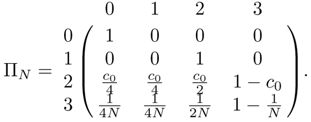(26)

Decomposing Π_N (eq. 26) into fast and slow transitions as in eq. 24, we can write matrices A and B as

$$\mathbf{A}=\left(\begin{array}{cccc}1& 0& 0& 0\\ 0& 0& 1& 0\\ \frac{c_0}{4}& \frac{c_0}{4}& \frac{c_0}{2}& 1-c_0\\ 0& 0& 0& 1\end{array}\right),\mathbf{B}=\left(\begin{array}{cccc}0& 0& 0& 0\\ 0& 0& 0& 0\\ 0& 0& 0& 0\\ \frac{1}{4}& \frac{1}{4}& \frac{1}{2}& -1\end{array}\right).$$ (27)

To find Π(t) we first derive the limit of matrix A. This computation, performed in Appendix A, gives

$$\mathbf{P}=\underset{r\to \infty }{\lim }{\mathbf{A}}^r=\left(\begin{array}{cccc}1& 0& 0& 0\\ \frac{c_0}{4-3c_0}& 0& 0& \frac{4-4c_0}{4-3c_0}\\ \frac{c_0}{4-3c_0}& 0& 0& \frac{4-4c_0}{4-3c_0}\\ 0& 0& 0& 1\end{array}\right).$$ (28)

Next, we compute the rate matrix G by taking the product

$$\mathbf{G}=\mathbf{PBP}=\left(\begin{array}{cccc}0& 0& 0& 0\\ \frac{4-4c_0}{{\left(4-3c_0\right)}^2}& 0& 0& -\frac{4-4c_0}{{\left(4-3c_0\right)}^2}\\ \frac{4-4c_0}{{\left(4-3c_0\right)}^2}& 0& 0& -\frac{4-4c_0}{{\left(4-3c_0\right)}^2}\\ \frac{1}{4-3c_0}& 0& 0& -\frac{1}{4-3c_0}\end{array}\right).$$

Finally, we apply eq. 25, computing the matrix exponential $\mathbf{\text{P}}{e}^{t\mathbf{G}}$. Converting t back to units of generations, we evaluate $\mathbf{P}{\sum }_{i=0}^{\infty }{(t/N)}^i{\mathbf{G}}^i/i!$,

$$\text{Π}(t)=\left(\begin{array}{cccc}1& 0& 0& 0\\ 1-\frac{4-4c_0}{4-3c_0}{e}^{\frac{-t}{N\left(4-3c_0\right)}}& 0& 0& \frac{4-4c_0}{4-3c_0}{e}^{\frac{-t}{N\left(4-3c_0\right)}}\\ 1-\frac{4-4c_0}{4-3c_0}{e}^{\frac{-t}{N\left(4-3c_0\right)}}& 0& 0& \frac{4-4c_0}{4-3c_0}{e}^{\frac{-t}{N\left(4-3c_0\right)}}\\ 1-e^{\frac{-t}{N\left(4-3c_0\right)}}& 0& 0& e^{\frac{-t}{N\left(4-3c_0\right)}}\end{array}\right).$$

From the bottom three rows of the first column of Π(t), corresponding to states 1, 2, and 3, respectively, we extract the limiting cumulative distribution functions for T, U, and V :

$$F_T(t)=F_U(t)=1-\frac{4-4c_0}{4-3c_0}{e}^{-\frac{t}{4N\left(1-\frac{3}{4}{c}_0\right)}}$$ (29)

$$F_V(t)=1-e^{-\frac{t}{4N\left(1-\frac{3}{4}{c}_0\right)}}.$$ (30)

We see in eq. 30 that V is exponentially distributed with mean $4N\left(1-\frac{3}{4}{c}_0\right)$, so that the coalescence time of two alleles in two individuals in separate mating pairs is distributed identically to that of two alleles in a standard haploid model with size $4N\left(1-\frac{3}{4}{c}_0\right)$. As $N\to \infty$ and $c_0\to 0$, $F_T(t)=F_V(t)$, and T, U, and V are all distributed identically to the coalescence time for two alleles in a haploid population of size 4N.

For c₀ > 0, T and U are not exponentially distributed. We have $F_T(t)-F_V(t)=\left[c_0/\left(4-3c_0\right)\right]e^{-t/\left[4N\left(1-\frac{3}{4}{c}_0\right)\right]}$, so $F_T(t)>F_V(t)$ and the probability that two alleles in an individual coalesce by t generations ago exceeds the corresponding probability for two alleles in separate mating pairs. As c₀ increases to 1 at fixed N and t, $F_T(t)-F_V(t)$ increases; for fixed N and c₀, the difference is largest at t = 0, decreasing to 0 as t increases.

From eqs. 29 and 30, noting that for a random variable X ≥ 0 with cumulative distribution function $F_X(x),\mathbb{E}[X]={\int }_{x=0}^{\infty }\left[1-F_X(x)\right]dx$ and $\mathbb{E}\left[X^2\right]={\int }_{x=0}^{\infty }2x\left[1-F_X(x)\right]dx$, we can compute the mean and variance of the limiting distributions of T and V as

$$\mathbb{E}\left[T_{\text{lim}}\right]=4N\left(1-c_0\right)$$ (31)

$$\mathbb{E}\left[V_{\text{lim}}\right]=4N\left(1-\frac{3}{4}{c}_0\right)$$ (32)

$$\text{Var}\left[T_{\text{lim}}\right]=16N^2\left(1-c_0\right)\left(1-\frac{1}{2}{c}_0\right)$$ (33)

$$\text{Var}\left[V_{\text{lim}}\right]=16N^2{\left(1-\frac{3}{4}{c}_0\right)}^2.$$ (34)

The differences between the large-N limiting values and the exact solutions in eqs. 1, 3, 11, and 12 are

$$\mathbb{E}[T]-\mathbb{E}\left[T_{\text{lim}}\right]=6$$ (35)

$$\mathbb{E}[V]-\mathbb{E}\left[V_{\text{lim}}\right]=4$$ (36)

$$\text{Var}[T]-\text{Var}\left[T_{\lim }\right]=28N\left(1-c_0\right)+22$$ (37)

$$\text{Var}[V]-\text{Var}\left[V_{\lim }\right]=28N\left(1-\frac{29}{28}{c}_0\right)+22.$$ (38)

For large N, the differences in eqs. 35–38 are negligible in comparison to the exact means and variances.

Eqs. 29 and 30 are plotted in Figure 3. In Figure 3A, we observe that as c₀ increases, the probability of instantaneous coalescence increases. This probability is maximized for c₀ = 1, where F_T(t) = 1, implying that all pairs of alleles coalesce quickly due to consanguinity. For V, we observe in Figure 3B that increased consanguinity decreases mean coalescence time $4N\left(1-\frac{3}{4}{c}_0\right)$, and the distribution behaves like a random-mating population with a reduced size. Compared to a haploid population of size 4N, for both T and V, as consanguinity increases, probability density is shifted towards zero, away from ancient coalescence times to more recent coalescence times.

Figure 3:

The cumulative distributions of coalescence times within (T) and between (V) individuals as functions of generations t and the fraction c₀ of sib mating pairs. (A) $\mathrm{\mathbb{P}}(T\le t)$, eq. 29. (B) $\mathrm{\mathbb{P}}(V\le t)$, eq. 30.

4.3. Superposition of multiple mating levels

We now generalize the separation-of-time-scales approach to allow a superposition of mating levels. Recall that under the superposition, ith-cousin mating is permitted for each i from 0 to n, where n is the degree of the most distant permissible cousin relationship. For each i, let c_i be the fraction of ith-cousin mating pairs each generation, with ${\sum }_{i=0}^n{c}_i\le 1$. As before, we assume that ith-cousin mating pairs are distinct sets for distinct i, such that two individuals in a mating pair cannot, for example, be both first and third cousins; this choice is suited to large populations with relatively low rates of consanguinity, so that ${\sum }_{i=0}^n{c}_i\ll 1$.

We derive the single-generation transition matrix Π_N. We have states 0, 1, and 3 as before, and transitions from these states are the same as under sib mating. For state 2, if two alleles are in two individuals in a mating pair in the current generation, then for each i, 0 ≤ i ≤ n, with probability c_i/4ⁱ, the two individuals are ith cousins and the alleles were inherited from the shared ancestral mating pair i + 1 generations in the past. For each i, 0 ≤ i ≤ n, there exists a state, which we call 2_i, that is visited i generations back in time from the current generation. For example, the state that we termed state 2 under sib mating we now call 2₀, because with probability c₀, the two individuals in the mating pair are 0th cousins (sibs) who share an ancestral mating pair 1 generation in the past. If two alleles have reached state 2_i, then they have not yet coalesced, and the two individuals in the current generation are not more closely related than ith cousins. If c_i > 0, then the individuals might be ith cousins and two alleles in state 2_i can be inherited from the shared ancestral mating pair in the next generation back in time from state 2_i (Figure 4).

Figure 4:

New states in the superposition model. Two alleles in two individuals who are in an ith cousin mating pair and have no closer relationship, i generations ago, are in separate mating pairs. We term their state i generations ago 2_i. In the next generation back, the alleles might be in the shared ancestral mating pair, as shown. Here, i = 2.

For convenience, for each i, 0 ≤ i ≤ n, we define k_i as the probability that two alleles in two individuals in a mating pair coalesce due to consanguinity in at most i + 1 generations, so that the individuals are ith cousins or more closely related,

$$k_i=\sum _{j=0}^i\frac{c_j}{4^{j+1}}.$$ (39)

We denote k₋₁ = 0. The probability that the alleles in two individuals in a mating pair reach a shared ancestral pair in at most i + 1 generations is $4k_i$; the conditional probability that they coalesce in that pair given that they have reached it is $\frac{1}{4}$. Then $1-4k_i$ is the probability that two alleles in two individuals in a mating pair are in a pair with relationship more distant than ith cousins; it is the probability that the individuals have no shared ancestor up to and including i + 1 generations back from the present.

We next define x_i for 0 ≤ i ≤ n as the conditional probability that two alleles in a mating pair are in an ith-cousin mating pair and that they coalesce in the shared ancestral pair i + 1 generations back, given that they have no shared ancestor i generations back or more recent. The probability that two alleles in a mating pair are in an ith-cousin pair is c_i, the probability that they coalesce in the shared ancestral pair is $1/4^{i+1}$, and the probability that they have no shared ancestor i generations back or more recent is $1-4k_{i-1}$. Hence,

$$x_i=\frac{c_i}{4^{i+1}\left(1-4k_{i-1}\right)}.$$ (40)

If two alleles are in state 2_i, then they are in lineages ancestral to two individuals who are not more closely related than ith cousins, and they have not coalesced. Two alleles in state 2_i have four possible transitions: with probability x_i, they coalesce (state 0); with probability x_i, they are inherited from the same individual in the ancestral mating pair but do not coalesce (state 1); with probability $2x_i$, they are inherited from two individuals in the ancestral mating pair (state 2₀). With probability $1-4x_i$, the two alleles were not inherited from a shared ancestor i + 1 generations ago, so the individuals in the current generation are not more closely related than (i + 1)th cousins, and the alleles transition to state 2_{i + 1}. If the alleles are in state 2_n, then they transition to states 0, 1, and 2₀, as seen for states 2_i, i < n, but the fourth transition is to two individuals in separate mating pairs (state 3), with probability $1-4x_n$.

Combining these cases gives the transition matrix ${\text{Π}}_N$ over states 0, 1, 3, and 2_i for $0\le i\le n$:

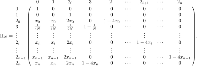(41)

Π_N decomposes into the $\mathcal{O}(1)$ transitions in matrix A,

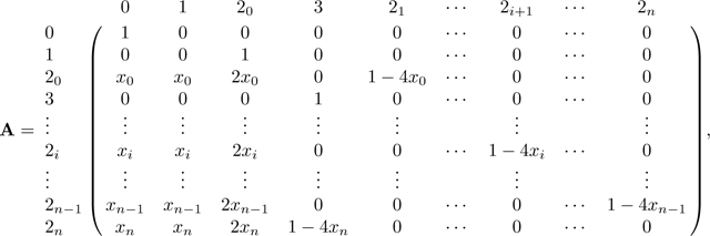(42)

and the $\mathcal{O}\left(\frac{1}{N}\right)$ transitions in matrix B,

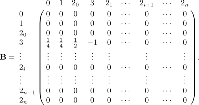(43)

We derive the equilibrium of A in Appendix B. We obtain

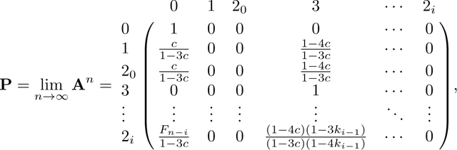(44)

where $F_{n-i}$ is described in Appendix B (P has the same dimension as A and B, but for convenience we do not expand down to rows 2_{n − 1} and 2_n in P, as they follow the form of row 2_i). Because A is an absorbing matrix with absorbing states 0 and 3, the only nonzero entries in P are in columns 0 and 3. Note that at equilibrium, ${\mathbf{P}}_{2_0,0}=\frac{c}{1-3c}=\frac{c}{c+1-4c}$. The numerator of this fraction is the probability that two alleles in a mating pair coalesce rapidly due to consanguinity, c, and the denominator is the sum of this quantity and the probability the two alleles are not inherited through the consanguineous pedigree, 1 − 4c. Note that for the sib mating case, c = c₀/4, and c/(1 − 3c) becomes c₀/(4 − 3c₀), as seen in eq. 28.

Next we take the product PBP (Appendix B) to find matrix G:

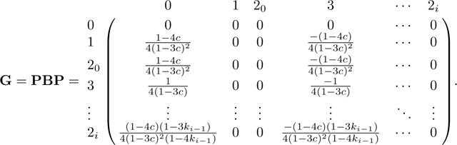(45)

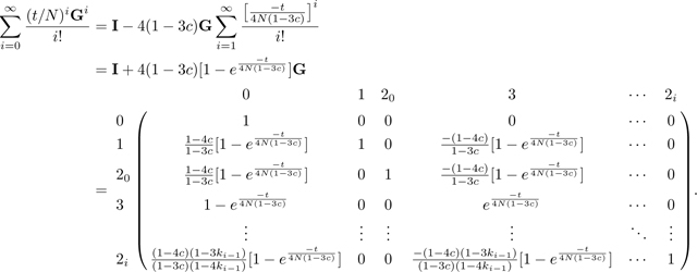
Lastly, to derive Π(t), we compute the exponential $e^{t\mathbf{G}}$ (Appendix B) and take the product $\mathbf{P}{e}^{t\mathbf{G}}$. With t measured in units of generations, we obtain

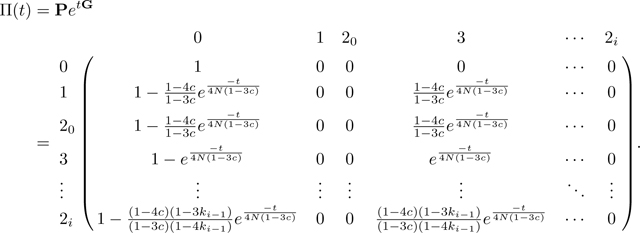(46)

As we observed for P, the only nonzero entries of Π(t) are in columns 0 and 3.

From column 0 of Π(t), examining the rows for states 1, 2₀, and 3, respectively, we have the limiting cumulative distributions for coalescence times T, U, and V :

$$F_T(t)=F_U(t)=1-\frac{1-4c}{1-3c}{e}^{-\frac{t}{4N(1-3c)}},$$ (47)

$$F_V(t)=1-e^{-\frac{t}{4N(1-3c)}}.$$ (48)

We immediately observe that for the sib mating case of c = c₀/4, eqs. 47 and 48 reduce to eqs. 29 and 30, respectively. In the limit, T and U are identically distributed but not exponential. The limiting V is exponentially distributed with mean 4N(1 − 3c); the coalescence time of two alleles in two individuals in separate mating pairs is therefore identically distributed with that of two alleles in a haploid population of size 4N(1 − 3c). Consanguinity reduces effective population size compared to random mating, with the reduction dependent on the kinship coefficient c of a randomly chosen mating pair.

The means and variances of the limiting distributions are

$$\mathbb{E}\left[T_{\text{lim}}\right]=4N(1-4c)$$ (49)

$$\mathbb{E}\left[V_{\text{lim}}\right]=4N(1-3c)$$ (50)

$$\text{Var}\left[T_{\text{lim}}\right]=16N^2(1-4c)(1-2c)$$ (51)

$$\text{Var}\left[V_{\lim }\right]=16N^2{(1-3c)}^2.$$ (52)

Considering eqs. 15 and 17, the differences between the exact and limiting means of T and V are

$$\mathbb{E}[T]-\mathbb{E}\left[T_{\text{lim}}\right]=4n(1-4c)+16d+6$$ (53)

$$\mathbb{E}[V]-\mathbb{E}\left[V_{\text{lim}}\right]=3n(1-4c)+12d+4.$$ (54)

The exact means exceed the limiting means for c > 0. Recall from Section 3.2 that $c\le \frac{1}{4}$, $d\le \frac{1}{16}$, and $b\le \frac{1}{16}$. Then for $n\ll N$, eqs. 53 and 54 contribute little to $\mathbb{E}[T]$ and $\mathbb{E}[V]$.

For the differences between the variances, we have

$$\begin{gathered} \text{Var}[T]-\text{Var}\left[T_{\text{lim}}\right]=4N(1-4c)(6n-16cn+16d+7) \\ +4n(1-4c)(3n-8cn+16d+8)+\left(128d^2+128d+16b+22\right) \end{gathered}$$ (55)

$$\begin{gathered} \text{Var}[V]-\text{Var}\left[V_{\lim }\right]=4N[(1-4c)(6n-18cn+18d+7)-c] \\ +4n(1-4c)(3n-9cn+18d+8)+\left(144d^2+128d+12b+22\right). \end{gathered}$$ (56)

For large N, because Var[T] and Var[V] are $\mathcal{O}\left(N^2\right)$, the differences contribute relatively little in relation to the magnitudes of the variances. Finally recall that if c = c₀/4, then d = 0, b = 0, and n = 0, and the quantities in eqs. 49–56 reduce to those for sib mating, eqs. 31–38.

For c = 0, there is no consanguinity, $F_T(t)=F_V(t)$, and T and V are both exponentially distributed. For c > 0, the difference $F_T(t)-F_V(t)=\frac{c}{1-3c}{e}^{-t/[4N(1-3c)]}$ is positive, and $F_T(t)>F_V(t)$. The probability that two alleles within an individual have coalesced by time t is greater than or equal to the probability for two alleles in separate individuals. As c increases to $\frac{1}{4}$, the difference increases; for fixed c, as t increases, the difference approaches zero, so that it is greatest for recent coalescence times.

5. Simulated distributions from the Markov chain

5.1. Simulation method

To examine the extent to which the limiting distributions of T and V accord with the exact distributions, we simulate pairwise coalescence times from the exact Markov chain (eq. 41). For both T and V, we consider a range of values of the number of mating pairs, N = 10,20,50,100,200,500,1000; the degree of cousin relationship, n = 0,1,2,3,4,5; and the consanguinity rate, c_n = 0,0.1,0.2,0.5,0.75. For simplicity, we consider only one type of cousin relationship at a time. For each of the two random variables, T and V, and each set of parameter values $\left\{N,n,c_n\right\}$, we simulated 10⁶ pairwise coalescence times.

To compare limiting distributions of coalescence times (eqs. 47 and 48) and simulated exact distributions, we compute a chi-square test statistic. We divide the limiting cumulative distribution functions into intervals and count occurrences of simulated coalescence times within those intervals. For V, we divide the limiting function into 50 intervals of equal probability 0.02. The limiting function for T is nonzero at t = 0; if the probability at 0 is 0.02 or greater, then the first interval is assigned size $f_T(0)$, and the remaining probability is divided into $q=\lfloor \left(1-f_T(0)\right)/0.02\rfloor$ intervals, each with size $\left(1-f_T(0)\right)/q\ge 0.02$.

5.2. Simulation results

The chi-square test statistics appear in Figure 5. Within each panel, we see that as N increases, the statistic generally decreases and then levels off, suggesting that increased population size improves the agreement between the exact and limiting distributions. This result accords with the fact that the limiting distribution is a large-N approximation, expected to more closely approximate the exact distribution as N increases.

Figure 5:

Values of the chi-square test statistic comparing the limiting distributions for T and V, eqs. 47 and 48, and the simulated exact distributions. The plots consider a range of values for the number of mating pairs (N), the consanguinity rate (c_n), and the degree of cousin relationship (n).

Considering the panels from left to right, as n increases past n = 1, the agreement is similar at different levels of consanguinity c_n. Thus, for relationships at the level of second or more distant cousins, the number of mating pairs N is the most important determinant of the agreement of the limiting and exact distributions. Examining the bottom row of Figure 5, for the random variable V, although for fixed N, the agreement is somewhat reduced at greater c_n, a key role for N is also observed for n = 0 and n = 1.

In the top row of Figure 5, for random variable T, we see that for n = 0 and n = 1, at high c_n, agreement between the limiting and exact distributions is relatively poor. In these cases, the probability of immediate coalescence in time 0 is larger in the limiting distribution. In the limiting distribution, with $c=c_n/4^{n+1}$, this probability is c/(1 − 3c) for f_T(0), and in the exact distribution, coalescence due to consanguinity has probability c. For large c, as occurs for large c₀ or c₁, $c/(1-3c)\not\approx c$.

In Figure 6, we more closely examine the effect of population size on the agreement between the limiting and simulated exact distributions. Over a range of population sizes, with n = 1 and a first-cousin relationship c₁ = 0.2, we plot the cumulative distribution functions of T and V for the first 4N generations. Considering plots from left to right, for both T and V, as N increases, the limiting distribution more closely matches the simulated exact distribution. In the small-N plots with N = 10, we can observe that the limiting distribution begins at t = 0 with a higher cumulative probability, and that this excess persists as t increases. Table 1 shows that the means and variances of T and V from the simulations accord closely with the exact theoretical means $\mathbb{E}[T]$ and $\mathbb{E}[V]$ (eqs. 15 and 17) and variances Var[T] and Var[V] (eqs. 22 and 23).

Figure 6:

Limiting cumulative distribution functions for T and V, eqs. 47 and 48, and simulated exact cumulative distributions, for 4N generations. The plots consider a range of values for the number of mating pairs (N), fixing the degree of cousin relationship at n = 1 and the consanguinity rate at c₁ = 0.2. (A) T, N = 10. (B) T, N = 100. (C) T, N = 1000. (D) T, N = 10000. (E) V, N = 10. (F) V, N = 100. (G) V, N = 1000. (H) V, N = 10000.

Table 1:

Agreement of the means and variances of T and V from the simulations in Figure 6 with the exact means for T and V (eqs. 15 and 17) and the exact variances (eqs. 22 and 23).

	N = 10		N = 100		N = 1000		N = 10000
	Exact	Simulated	Exact	Simulated	Exact	Simulated	Exact	Simulated
$\mathbb{E}[T]$	48	45	385	387	3760	3809	37510	37973
Var[T]	2.01 × 103	2.04 × 103	1.50 × 105	1.54 × 105	1.46 × 107	1.49 × 107	1.45 × 109	1.48 × 109
$\mathbb{E}[V]$	45	46	388	392	3820	3849	38132	38491
Var[V]	2.01 × 103	2.04 × 103	1.50 × 105	1.54 × 105	1.46 × 107	1.48 × 107	1.45 × 109	1.48 × 109

In WAKELEY et al. (2012), the disagreement between coalescence time distributions for two models, a pedigree model with N individuals and the Kingman coalescent, was greatest in the most recent log₂(N) generations. As our consanguinity models are similar to the pedigree model in that consanguinity influences the probability of rapid coalescence, we next examined the agreement of the limiting and simulated exact coalescent time distributions in the most recent generations. With the same parameter values as in Figure 6, Figure 7 focuses on the first 25 generations. For T, in Figure 7A-D, a difference occurs between the limiting and simulated exact distributions during the most recent generations, as the limiting distribution has a point mass at t = 0. For V, in Figure 7E-H, the limiting distribution does not have a point mass at t = 0, and the distributions differ by an amount that is approximately constant over the first 25 generations.

Figure 7:

Limiting cumulative distribution functions for T and V, eqs. 47 and 48, and simulated exact cumulative distributions, for 25 generations. The plots consider a range of values for the number of mating pairs (N), fixing the degree of cousin relationship at n = 1 and the consanguinity rate at c₁ = 0.2. (A) T, N = 10. (B) T, N = 100. (C) T, N = 1000. (D) T, N = 10000. (E) V, N = 10. (F) V, N = 100. (G) V, N = 1000. (H) V, N = 10000.

6. Discussion

Building on a study of mean coalescence times under consanguinity in a diploid model with N mating pairs, we have expanded the analysis to examine full coalescence time distributions. Under sib mating, we calculated the exact variance of coalescence times for two alleles within an individual and two alleles in separate individuals (eqs. 11 and 12), and we generalized the result to a superposition of multiple levels of cousin mating (eqs. 22 and 23). Using separation of time scales to examine “fast” coalescence by consanguinity and “slow” coalescence in the general population, we derived the large-N limiting distribution of pairwise coalescence times for two alleles within an individual and two alleles in separate individuals, in both the sib mating (eqs. 29 and 30) and superposition models (eqs. 47 and 48). As N increases, distributions simulated from the exact Markov chain approach the limiting distributions (Figures 5–7).

Previously (SEVERSON et al., 2019), we showed that increased consanguinity reduces mean pairwise coalescence times both within and between individuals, with a stronger effect for two alleles within an individual. In each of several models, we found that the reduction factor could be written in terms of the kinship coefficient c of a randomly chosen mating pair. Here, by deriving limiting distributions of coalescence times, we can further explain the earlier result. In particular, for two alleles in separate individuals, limiting coalescence times are distributed with pairwise coalescence times as in a haploid population of size 4N(1 − 3c). For two alleles within an individual, the distribution is a mixture of this effective size reduction and instantaneous coalescence with probability $\frac{c}{1-3c}$. Increasing consanguinity reduces the coalescent effective size (SJÖDIN et al., 2005) of the “slow” process; in the large-N limit, if rapid coalescence due to consanguinity does not occur, then coalescence follows the standard haploid model with the reduced population size.

The view of our model as having rapid coalescence due to consanguinity followed by coalescence mimicking a standard haploid population aligns with similar results for other phenomena that permit the separation-of-time-scales approach (WAKELEY, 2009, chapter 6). Related models consider partial selfing (NORDBORG and DONNELLY, 1997; MÖHLE, 1998b; NORDBORG and KRONE, 2002), two sexes (MÖHLE, 1998a; NORDBORG and KRONE, 2002), stage structure (NORDBORG and KRONE, 2002), many-demes migration (WAKELEY, 2001, 2004; ELDON and WAKELEY, 2009), and combinations of factors, as in an analysis of two sexes, sex chromosomes, and migration (RAMACHANDRAN et al., 2008).

The parallel is most natural for partial selfing. Following NORDBORG and KRONE (2002), consider a diploid population of 2N individuals, in which the probability that two alleles within an individual coalesce in the previous generation is $\frac{s}{2}$, where s is the selfing rate—the fraction of individuals for whom the same parent provides both of their genomic copies. In the selfing model, $\frac{s}{2}$ is the probability of immediate coalescence in one generation, and 1 − s is the probability that a pair of alleles “escapes” from the rapid time scale of coalescence by selfing. In the large-N limit, the probability of rapid coalescence is $\left(\frac{s}{2}\right)/\left(\frac{s}{2}+1-s\right)=\frac{s}{2-s}$. This result has a similar structure to our large-N result that the probability of rapid coalescence by consanguinity for two alleles in a mating pair is $\frac{c}{c+1-4c}=\frac{c}{1-3c}$, where c is the probability of coalescence by consanguinity during the first n generations and 1 − 4c is the probability of escape into the slow process. In both cases, a probability exists that the alleles return to the initial configuration—$\frac{s}{2}$ for the selfing model and 3c for the consanguinity model—with the chance to either coalesce in the fast process or escape to the slow one.

Chang (1999) modeled a biparental population of size N diploid individuals, finding that with high probability, all individuals in the population share a genealogical ancestor log₂ N generations ago. Extensions have sought to determine the effect of inbreeding on this result (LACHANCE, 2009), to estimate the timing of the most recent genealogical ancestor for all human individuals (ROHDE et al., 2004), and to further understand the relationship between genealogical and genetic ancestry in pedigrees (MATSEN and EVANS, 2008; GRAVEL and STEEL, 2015). WAKELEY et al. (2012, 2016) studied the distribution of coalescence times in models with pedigrees, finding that the effect of the pedigree dissipates farther back in time than the most recent log₂ N generations in a population of N diploid individuals. Recent extensions have considered population structure in coalescent models with pedigrees (KELLEHER et al., 2016; WILTON et al., 2017) and the effect of the population pedigree on coalescent-based parameter estimation (KING et al., 2018). Within this context, the current study and our earlier SEVERSON et al. (2019) contribute to a growing body of research integrating coalescent perspectives with genealogical studies of pedigrees.

We have described a superposition of multiple levels of cousin mating, where ith cousin mating can occur for each i, 0 ≤ i ≤ n, with c_i being the fraction of ith cousin mating pairs. We assumed that in a given generation, each mating pair can be in at most one category of ith cousins, so that $\sum c_i\le 1$. Thus, we track if alleles from a consanguineous mating pair representing ith cousins coalesce in the single shared mating pair that is modeled. This approach is suited to a large population with relatively low rates of consanguinity, where the probability is low that two individuals in a mating pair share multiple recent lines of descent.

In principle, however, the single shared ancestral mating pair of a consanguineous pair in the current generation can itself be a consanguineous pair. Depending on the level of relationship of these consanguineous pairs, the pair in the current generation could potentially share more than one line of descent in the most recent n generations. The Markov chain in eq. 41 only explicitly models the most recent of these lines of descent; it follows lineages backward in time, tracking if they have reached the single shared ancestral mating pair. Thus, in each generation, c_i is the fraction of mating pairs that are at least ith cousins, but that could also share additional, more distant lines of descent. If the c_i are low, then it is unlikely that consanguinity would compound in this manner in the most recent n generations. However, if the c_i become larger, then such cases are non-negligible. Our simulations focused on cases with a single form of consanguinity; to assess the possible lack of fit of the model owing to a compounding of consanguinity within the most recent n generations, it will be useful to simulate examples in which multiple forms of consanguinity occur at non-negligible levels.

Our interest in studying coalescence time in a consanguinity model has been motivated by the link between coalescence times and lengths of genomic segments shared identically by descent, with the random variable T connecting to ROH within individuals, and V connecting to IBD tracts between genomes in separate individuals chosen at random in a population (SEVERSON et al., 2019). For a pair of genomes, the random length of the segment shared identically by descent around a locus is inversely related to the random pairwise coalescence time at the focal locus, with recombination acting to shorten the shared fragment. In our previous work (SEVERSON et al., 2019), we used the inverse relationship between the mean coalescence time and shared fragment length to provide qualitative results on trends in ROH and IBD sharing in relation to consanguinity. Under a recombination model, the distribution of the shared fragment length can be obtained from the full distribution of pairwise coalescence times (PALAMARA et al., 2012; CARMI et al., 2013, 2014). As we have now obtained the limiting distributions of pairwise coalescence times, both within and between individuals, it will now be possible to deepen empirical analyses of the effect of consanguinity on patterns in shared genomic segments.

Appendix A. Sib mating

For sib mating, this appendix provides details of the computation of matrix P, the r → ∞ limit of A^r. The matrix A appears in eq. 27. To find the desired limit, note that A is an absorbing matrix with absorbing states 0 and 3. Recall that for an absorbing matrix D with form

$$\mathbf{D}=\left(\begin{array}{cc}\mathbf{I}& 0\\ \mathbf{R}& \mathbf{\text{Q}}\end{array}\right),$$

and with fundamental matrix $\mathbf{N}={(\mathbf{I}-\mathbf{Q})}^{-1}$, the limit of D^r is given by

$$\underset{r\to \infty }{\lim }{\mathbf{D}}^r=\left(\begin{array}{cc}\mathbf{I}& 0\\ \mathbf{NR}& 0\end{array}\right).$$ (57)

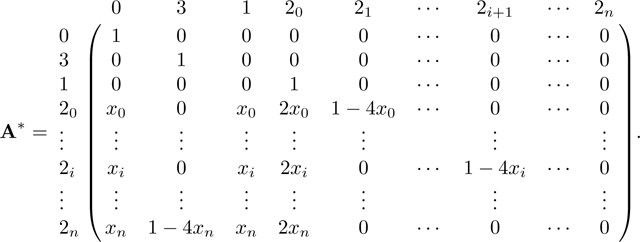
We rearrange A to match the form of D by permuting rows and columns to obtain permuted matrix A*:

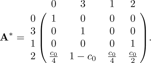Now we can read R and Q as

$$\mathbf{R}=\left(\begin{array}{cc}0& 0\\ \frac{c_0}{4}& 1-c_0\end{array}\right),\mathbf{Q}=\left(\begin{array}{cc}0& 1\\ \frac{c_0}{4}& \frac{c_0}{2}\end{array}\right).$$

Next we compute the fundamental matrix N:

$$\mathbf{N}={(\mathbf{I}-\mathbf{Q})}^{-1}=\left(\begin{array}{c}\frac{4-2c_0}{4-3c_0}\frac{4}{4-3c_0}\\ \frac{c_0}{4-3c_0}\frac{4}{4-3c_0}\end{array}\right).$$

We find the product NR:

$$\mathbf{NR}=\left(\begin{array}{cc}\frac{c_0}{4-3c_0}& \frac{4-4c_0}{4-3c_0}\\ \frac{c_0}{4-3c_0}& \frac{4-4c_0}{4-3c_0}\end{array}\right).$$

Following eq. 57, we have the desired limit,

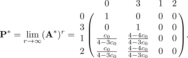Permuting the columns and rows again, we obtain eq. 28.

Appendix B. Superposition of multiple mating levels

This appendix provides details of the separation-of-time-scales computations in the case of a superposition of mating levels. We begin with some lemmas.

Two lemmas

We recall k_i and x_i from eqs. 39 and 40. First, we will need a recursion F, defined by $F_0=x_n$ and $F_m=x_{n-m}+\left(1-4x_{n-m}\right)F_{m-1}$ for m ≥ 1.

Lemma 1.

For m ≥ 1,

$$F_m=\frac{k_n-k_{n-m-1}}{1-4k_{n-m-1}}.$$

Proof:

First consider the base case m = 0,

$$F_0=x_n=\frac{c_n}{4^{n+1}\left(1-4k_{n-1}\right)}=\frac{k_n-k_{n-1}}{1-4k_{n-1}}.$$

Next, we assume for induction that $F_{m-1}=\left(k_n-k_{n-m}\right)/\left(1-4k_{n-m}\right)$. Then

$$\begin{array}{l}{F}_m=x_{n-m}+\left(1-4x_{n-m}\right)F_{m-1}\\ =\frac{c_{n-m}}{4^{n-m+1}\left(1-4k_{n-m-1}\right)}+\left[1-\frac{4c_{n-m}}{4^{n-m+1}\left(1-4k_{n-m-1}\right)}\right]\left(\frac{k_n-k_{n-m}}{1-4k_{n-m}}\right)\\ =\frac{k_{n-m}-k_{n-m-1}}{1-4k_{n-m-1}}+\left(\frac{1-4k_{n-m}}{1-4k_{n-m-1}}\right)\left(\frac{k_n-k_{n-m}}{1-4k_{n-m}}\right)\\ =\frac{k_n-k_{n-m-1}}{1-4k_{n-m-1}}.\end{array}$$

This completes the proof. □

Lemma 2.

For $\ell \ge j\ge 0$,

$$\prod _{i=j}^{\ell }\left(1-4x_i\right)=\frac{1-4k_{\ell }}{1-4k_{j-1}}.$$

Proof:

We use $c_i/4^{i+1}=k_i-k_{i-1}$ from eq. 39:

$$\prod _{i=j}^{\ell }\left(1-4x_i\right)=\prod _{i=j}^{\ell }\left[1-\frac{c_i}{4^i\left(1-4k_{i-1}\right)}\right]=\prod _{i=j}^{\ell }\left(\frac{1-4k_i}{1-4k_{i-1}}\right)=\frac{1-4k_{\ell }}{1-4k_{j-1}}.\square$$

The limiting matrix P

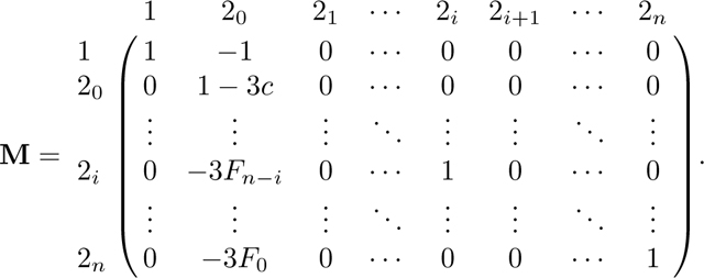
We follow the same method as in Appendix A. Again because A has two absorbing states, 0 and 3, we can derive the equilibrium matrix P with eq. 57. Permuting the columns and rows of A in eq. 42 from $\left(0,1,2_0,3,\dots ,2_i,\dots ,2_n\right)$ to $\left(0,3,1,2_0,\dots ,2_i,\dots ,2_n\right)$, A* has form

From A*, we find R and Q as

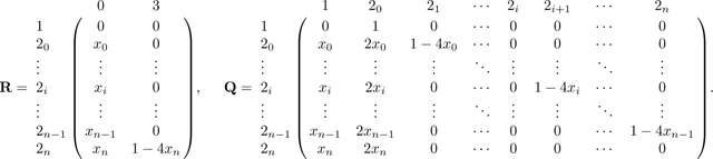(58)

First, we find the fundamental matrix N = (I − Q)⁻¹. We proceed by Gaussian elimination, beginning from the augmented matrix [(I − Q)| I] and proceeding to obtain (I|N). We write M = I − Q:

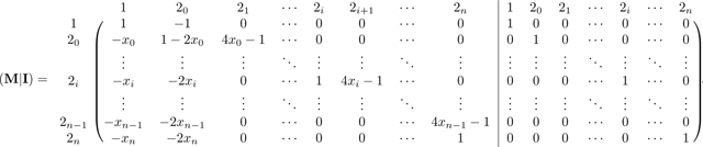For convenience, we refer to rows and columns of M and N by their associated states, and continue to refer to the left and right components of the augmented matrix by M and N.

To begin the elimination, for each row 2_i we eliminate $-x_i$ in the first column by adding x_i times row 1. As this step leaves a value of $4x_{n-1}-1$ in column $2_n$ of matrix M, we next add $1-4x_{n-1}$ times row 2_n to row $2_{n-1}$, obtaining

Notice that in M, for each row 2i for i from 0 to n − 2, the entry in column 2_{i + 1} satisfies ${\mathbf{M}}_{2_i,2_{i+1}}=4x_i-1$. Now that we have eliminated $4x_{n-1}-1$ in row $2_{n-1}$, we repeat the same operation and use row $2_{n-1}$ to eliminate $4x_{n-2}-1$ in the row above, $2_{n-2}$. Specifically, we add $\left(1-4x_{n-2}\right){\mathbf{M}}_{2_{n-1},•}$ to ${\mathbf{M}}_{2_{n-2},•}$ (where $•$ indicates that here we consider row vectors). Decrementing i from n − 2 to 0, for each i, we perform this operation of adding to row 2_i the quantity $\left(1-4x_i\right){\mathbf{M}}_{2_{i+1},•}$. Repeatedly performing this operation produces a recursion in column 2₀, and we have

The operation of successively adding $\left(1-4x_i\right){\mathbf{N}}_{2_{i+1},•}$ to ${\mathbf{N}}_{2_i,•}$ also produces the recursion F in column 1 of N. This operation creates increasing products of terms $1-4x_i$ in the upper right triangle of N. For an entry ${\mathbf{N}}_{2_j,2_{\ell }}$, with $\ell >j$, the entry is given by the product ${\prod }_{i=j}^{\ell }\left(1-4x_i\right)$. After completing this operation for all rows 2_i in N, $0\le i\le n-1$, the matrix is

We can now simplify matrices M and N using Lemmas 1 and 2. First, by Lemma 1, $F_n=\left(k_n-k_{-1}\right)/\left(1-4k_{-1}\right)=k_n=c$, where c, defined in eq. 18, is the kinship coefficient of two individuals in a randomly chosen mating pair. Then we can rewrite M as

Using Lemma 2, we can simplify N:

For the last elimination step in column 2₀ of M, we first divide row 2₀ of M and N by 1 − 3c and then add the resulting row 2₀ to row 1. We obtain:

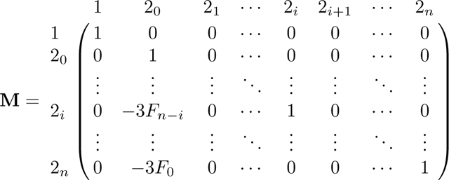
Next, for each remaining row $2_i,1\le i\le n$, in M, we add $3F_{n-i}$ times row 2₀, which for M gives

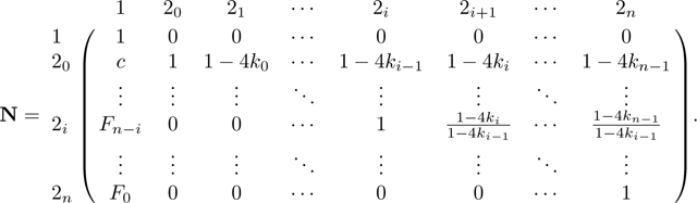
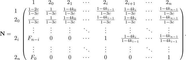
For N, this step produces the fundamental matrix N = (I − Q)⁻¹, with form

$${\mathbf{N}}_{1,•}=\left[\frac{1-2c}{1-3c},\frac{1}{1-3c},\frac{1-4k_0}{1-3c},\dots ,\frac{1-4k_{n-1}}{1-3c}\right]$$

$${\mathbf{N}}_{2_0,•}=\left[\frac{c}{1-3c},\frac{1}{1-3c},\frac{1-4k_0}{1-3c},\dots ,\frac{1-4k_{n-1}}{1-3c}\right]$$

$${\mathbf{N}}_{2_i,•}=3F_{n-i}{\mathbf{N}}_{2_0,•}+\left[F_{n-i},0,\dots ,1,\frac{1-4k_i}{1-4k_{i-1}},\dots ,\frac{1-4k_{n-1}}{1-4k_{i-1}}\right],1\le i\le n.$$

Now that we have derived the fundamental matrix N, we next find the product NR. From eq. 58,

$${\mathbf{R}}_{•,0}={\left[0,x_0,\dots ,x_n\right]}^T$$

$${\mathbf{R}}_{•,3}={\left[0,\dots ,0,1-4x_n\right]}^T.$$

Because ${\mathbf{R}}_{1,•}=[0,0]$ and rows ${\mathbf{N}}_{1,•}$ and ${\mathbf{N}}_{2_0,•}$ only differ at their first entry, we have dot products ${\mathbf{\text{N}}}_{1,•}\cdot {\mathbf{R}}_{•,0}={\mathbf{N}}_{2_0,•}\cdot {\mathbf{R}}_{•,0}$ and ${\mathbf{N}}_{1,•}\cdot {\mathbf{R}}_{•,3}={\mathbf{N}}_{20,•}\cdot {\mathbf{R}}_{•,3}$. Hence, to complete the derivation of NR, it suffices to compute the dot products of ${\mathbf{N}}_{1,•}$ and ${\mathbf{N}}_{2_i,•}$, 1 ≤ i ≤ n, with ${\mathbf{R}}_{•,0}$ and ${\mathbf{R}}_{•,3}$. Using eqs. 39 and 40 and Lemma 1, these products are

$$\begin{array}{l}{\mathbf{N}}_{1,•}\cdot {\mathbf{R}}_{•,0}=\frac{1}{1-3c}\sum _{i=0}^n{x}_i\left(1-4k_{i-1}\right)\\ =\frac{1}{1-3c}\sum _{i=0}^n\frac{c_i\left(1-4k_{i-1}\right)}{4^{i+1}\left(1-4k_{i-1}\right)}\\ =\frac{c}{1-3c}.\end{array}$$

$$\begin{gathered} {\mathbf{N}}_{2_i,•}\cdot {\mathbf{R}}_{•,0}=\frac{3c{F}_{n-i}}{1-3c}+\sum _{j=i}^n\frac{x_j\left(1-4k_{j-1}\right)}{1-4k_{i-1}} \\ =\frac{3c{F}_{n-i}}{1-3c}+\frac{1}{1-4k_{i-1}}\sum _{j=i}^n\frac{c_j\left(1-4k_{j-1}\right)}{4^{j+1}\left(1-4k_{j-1}\right)} \\ =\frac{3c{F}_{n-i}}{1-3c}+\frac{k_n-k_{i-1}}{1-4k_{i-1}} \\ =\frac{F_{n-i}}{1-3c}. \end{gathered}$$

$$\begin{gathered} {\mathbf{N}}_{1,•}\cdot {\mathbf{R}}_{•,3}=\frac{1-4k_{n-1}}{1-3c}\left(1-4x_n\right) \\ =\frac{1-4k_{n-1}}{1-3c}\frac{1-4k_n}{1-4k_{n-1}} \\ =\frac{1-4c}{1-3c}. \end{gathered}$$

$$\begin{array}{l}{\mathbf{N}}_{2^i,•}\cdot {\mathbf{R}}_{•,3}=\frac{3F_{n-i}(1-4c)}{1-3c}+\frac{\left(1-4k_{n-1}\right)\left(1-4x_n\right)}{1-4k_{i-1}}\\ =\frac{3\left(k_n-k_{i-1}\right)(1-4c)}{\left(1-4k_{i-1}\right)(1-3c)}+\frac{\left(1-4k_{n-1}\right)\left(1-4k_n\right)}{\left(1-4k_{i-1}\right)\left(1-4k_{n-1}\right)}\\ =\frac{(1-4c)\left(1-3k_{i-1}\right)}{(1-3c)\left(1-4k_{i-1}\right)}.\end{array}$$

Combining these cases, we find

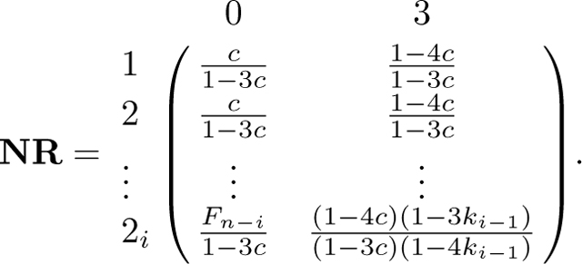We have

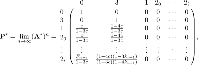from which we obtain P in eq. 44 by permuting rows and columns.

The generator matrix G

Here we derive the generator matrix G=PBP. Recall B from eq. 43. We first compute BP.

Because ${\mathbf{\text{B}}}_{3,•}$ is the only nonzero row of B, the only nonzero row of BP is ${(\mathbf{\text{BP}})}_{3,•}$. Similarly, because columns ${\mathbf{\text{P}}}_{•,0}$ and ${\mathbf{\text{P}}}_{•,3}$ are the only nonzero columns of P, the only nonzero columns of BP are ${(\mathbf{BP})}_{•,0}$ and ${(\mathbf{\text{BP}})}_{•,3}$. Therefore the only nonzero entries of BP are (BP)_3,0 and (BP)_3,3:

$${\mathbf{B}}_{3,•}\cdot {\mathbf{P}}_{•,0}=\frac{1}{4}+\frac{3c}{4(1-3c)}=\frac{1}{4(1-3c)}$$

$${\mathbf{B}}_{3,•}\cdot {\mathbf{P}}_{•,3}=\frac{3(1-4c)}{4(1-3c)}-1=\frac{-1}{4(1-3c)}.$$

Hence, we have

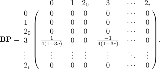Next, for the product PBP, we note again that because only columns ${(\mathbf{\text{BP}})}_{•,0}$ and ${(\mathbf{\text{BP}})}_{•,3}$ are nonzero, the only nonzero columns of PBP are 0 and 3. Because the only nonzero elements of columns ${(\mathbf{\text{BP}})}_{•,0}$ and ${(\mathbf{\text{BP}})}_{•,3}$ are in row ${(\mathbf{BP})}_{3,•}$, the entries in columns ${(\mathbf{\text{PBP}})}_{•,0}$ and ${(\mathbf{\text{PBP}})}_{•,3}$ are the products of entries in column ${\mathbf{\text{P}}}_{•,3}$ and ${(\mathbf{\text{BP}})}_{•,0}$ or ${(\mathbf{\text{BP}})}_{•,3}$. In other words, the nonzero columns of PBP are

$${(\mathbf{PBP})}_{•,0}=\frac{1}{4(1-3c)}{\mathbf{P}}_{•,3}$$

$${(\mathbf{PBP})}_{•,3}=\frac{-1}{4(1-3c)}{\mathbf{P}}_{•,3}$$

The generating matrix is given by G=PBP as in eq. 45.

The matrix exponential Π(t)

To compute the exponential $e^{t\mathbf{G}}$, we first note that ${\mathbf{G}}^2=-\mathbf{G}/[4(1-3c)]$. In general, for n > 0,

$${\mathbf{G}}^n={\left[\frac{-1}{4(1-3c)}\right]}^{n-1}\mathbf{\text{G}}.$$

We can then derive the matrix exponential $e^{t\mathbf{G}}$, converting t to units of generations:

We take the product $\mathbf{P}{e}^{t\mathbf{G}}$, using eq. 44 for P, to produce Π(t), eq. 46.

References

- CAMPBELL RB, 2015The effect of inbreeding constraints and offspring distribution on time to the most recent common ancestor. Journal of Theoretical Biology 382: 74–80. [DOI] [PubMed] [Google Scholar]
- CARMI S, PALAMARA PF, VACIC V, LENCZ T, DARVASI A, et al. , 2013The variance of identity-by-descent sharing in the Wright-Fisher model. Genetics 193: 911–928. [DOI] [PMC free article] [PubMed] [Google Scholar]
- CARMI S, WILTON PR, WAKELEY J, and PE’ER I, 2014A renewal theory approach to IBD sharing. Theoretical Population Biology 97: 35–48. [DOI] [PMC free article] [PubMed] [Google Scholar]
- CHANG JT, 1999Recent common ancestors of all present-day individuals. Advances in Applied Probability 31: 1002–1026. [Google Scholar]
- ELDON B, and WAKELEY J, 2009Coalescence times and FST under a skewed offspring distribution among individuals in a population. Genetics 181: 615–629. [DOI] [PMC free article] [PubMed] [Google Scholar]
- GRAVEL S, and STEEL M, 2015The existence and abundance of ghost ancestors in biparental populations. Theoretical Population Biology 101: 47–53. [DOI] [PubMed] [Google Scholar]
- KELLEHER J, ETHERIDGE AM, VÉBER A, and BARTON NH, 2016Spread of pedigree versus genetic ancestry in spatially distributed populations. Theoretical Population Biology 108: 1–12. [DOI] [PubMed] [Google Scholar]
- KING L, WAKELEY J, and CARMI S, 2018A non-zero variance of Tajima’s estimator for two sequences even for infinitely many unliked loci. Theoretical Population Biology 122: 22–29. [DOI] [PubMed] [Google Scholar]
- LACHANCE J, 2009Inbreeding, pedigree size, and the most recent common ancestor of humanity. Journal of Theoretical Biology 261: 238–247. [DOI] [PMC free article] [PubMed] [Google Scholar]
- MATSEN FA, and EVANS SN, 2008To what extent does genealogical ancestry imply genetic ancestry? Theoretical Population Biology 74: 182–190. [DOI] [PubMed] [Google Scholar]
- MÖHLE M, 1998aCoalescent results for two-sex population models. Advances in Applied Probability 30: 513–520. [Google Scholar]
- mÖHLE M, 1998bA convergence theorem for Markov chains arising in population genetics and the coalescent with selfing. Advances in Applied Probability 30: 493–512. [Google Scholar]
- NORDBORG M, and DONNELLY P, 1997The coalescent process with selfing. Genetics 146: 1185–1195. [DOI] [PMC free article] [PubMed] [Google Scholar]
- NORDBORG M, and KRONE SM, 2002Separation of time scales and convergence to the coalescent in structured populations. In Slatkin M. and Veuille M, editors, Modern Developments in Theoretical Population Genetics, chapter 12. Oxford University Press, Oxford, 194–232. [Google Scholar]
- PALAMARA PF, LENCZ T, DARVASI A, and PE’ER I, 2012Length distributions of identity by descent reveal fine-scale demographic history. American Journal of Human Genetics 91: 809–822. [DOI] [PMC free article] [PubMed] [Google Scholar]
- RAMACHANDRAN S, ROSENBERG NA, FELDMAN MW, and WAKELEY J, 2008Population differentiation and migration: coalescence times in a two-sex island model for autosomal and X-linked loci. Theoretical Population Biology 74: 291–301. [DOI] [PMC free article] [PubMed] [Google Scholar]
- ROHDE DL, OLSON S, and CHANG JT, 2004Modelling the recent common ancestry of all living humans. Nature 431: 562. [DOI] [PubMed] [Google Scholar]
- SEVERSON AL, CARMI S, and ROSENBERG NA, 2019The effect of consanguinity on between-individual identity-by-descent sharing. Genetics 212: 305–316. [DOI] [PMC free article] [PubMed] [Google Scholar]
- SJODIN P, KAJ I, KRONE S, LASCOUX M, and NORDBORG M, 2005On the meaning and existence of an effective population size. Genetics 169: 1061–1070. [DOI] [PMC free article] [PubMed] [Google Scholar]
- WAKELEY J, 2001The coalescent in an island model of population subdivision with variation among demes. Theoretical Population Biology 59: 133–144. [DOI] [PubMed] [Google Scholar]
- WAKELEY J, 2004Metapopulation models for historical inference. Molecular Ecology 13: 865–875. [DOI] [PubMed] [Google Scholar]
- WAKELEY J, 2009Coalescent Theory: An Introduction. Roberts & Company, Greenwood Village, CO. [Google Scholar]
- WAKELEY J, KING L, Low BS, and RAMAOHANDRAN S, 2012Gene genealogies within a fixed pedigree, and the robustness of Kingman’s coalescent. Genetics 190: 1433–1445. [DOI] [PMC free article] [PubMed] [Google Scholar]
- WAKELEY J, KING L, and WILTON PR, 2016Effects of the population pedigree on genetic signatures of historical demographic events. Proceedings of the National Academy of Sciences USA 113: 7994–8001. [DOI] [PMC free article] [PubMed] [Google Scholar]
- WILTON PR, BADUEL P, LANDON MM, and WAKELEY J, 2017Population structure and coalescence in pedigrees: Comparisons to the structured coalescent and a framework for inference. Theoretical Population Biology 115: 1–12. [DOI] [PubMed] [Google Scholar]