Evaluating a Convolutional Neural Network Noise Reduction Method When Applied to CT Images Reconstructed Differently Than Training Data

Abstract

Objective:

The aim of this study was to evaluate a narrowly trained convolutional neural network (CNN) denoising algorithm when applied to images reconstructed differently than training data set.

Methods:

A residual CNN was trained using 10 noise inserted examinations. Training images were reconstructed with 275 mm of field of view (FOV), medium smooth kernel (D30), and 3 mm of thickness. Six examinations were reserved for testing; these were reconstructed with 100 to 450 mm of FOV, smooth to sharp kernels, and 1 to 5 mm of thickness.

Results:

When test and training reconstruction settings were not matched, there was either reduced denoising efficiency or resolution degradation. Denoising efficiency was reduced when FOV was decreased or a smoother kernel was used. Resolution loss occurred when the network was applied to an increased FOV, sharper kernel, or decreased image thickness.

Conclusions:

The CNN denoising performance was degraded with variations in FOV, kernel, or decreased thickness. Denoising performance was not affected by increased thickness.

Clinical computed tomography (CT) uses x-ray radiation to generate image representations of internal anatomic structures. To reduce patient risk, it is best practice to lower radiation dose as much as possible without compromising image quality.^1,2

Decreased radiation exposure during CT typically leads to increased image noise, potentially resulting in decreased reader performance and increased reader fatigue.³ Multiple noise reduction techniques have been developed, including iterative reconstruction^4,5 and various projection-space and image-space denoising methods.^6–9 Recently, deep learning–based methods using convolutional neural networks (CNNs) have attracted interest because of their powerful denoising capabilities and computational efficiency. Such CNN models have been applied to denoising tasks on natural images^10–12 and proposed for medical image denoising.¹³

Although the use of CNN-based denoising techniques shows great promise for improving the interpretability of medical images, unique challenges are associated with this approach. Many of these challenges can be attributed to the absence of a priori analytic rules with CNN-based denoising. Instead, CNN denoising is achieved by minimizing a loss function evaluated on a particular set of training data. Training data typically consist of pairs of high-noise (input) images and corresponding low-noise (target) images. After the model is optimized, or “trained,” the abstract rules used by the CNN to separate signal from noise are generally not human interpretable, making it difficult to anticipate how the algorithm will perform in different scenarios. Furthermore, the rules used by the CNN depend strongly on the particular sample of training images, which may limit the extent to which the algorithm can be used in a broad clinical context. This broad clinical context includes natural difference of human anatomy, various acquisition parameters (tube potential and current, focal spot size, beam filtering, angular sampling, and detector specifications), and reconstruction settings (field of view [FOV], kernel, and image thickness). It is critical to evaluate CNN-based denoising algorithms in response to this parameter space.

This study explored the reconstruction generalizability of a narrowly trained CNN-based denoising algorithm to better understand the potential boundaries on the applicability of such techniques to CT images in a general clinical context. Specifically, we examined how well the denoising model generalized when applied to images reconstructed with conditions different from those used during training. This work characterized the degree to which performance was degraded for clinically relevant differences in the reconstruction conditions.

MATERIALS AND METHODS

Residual CNN Architecture

A deep residual CNN architecture (Fig. 1) was used as a model that maps input CT images to a predicted low-noise output image. This architecture was implemented similarly to ResNet and ResNeXt.^14,15

FIGURE 1.

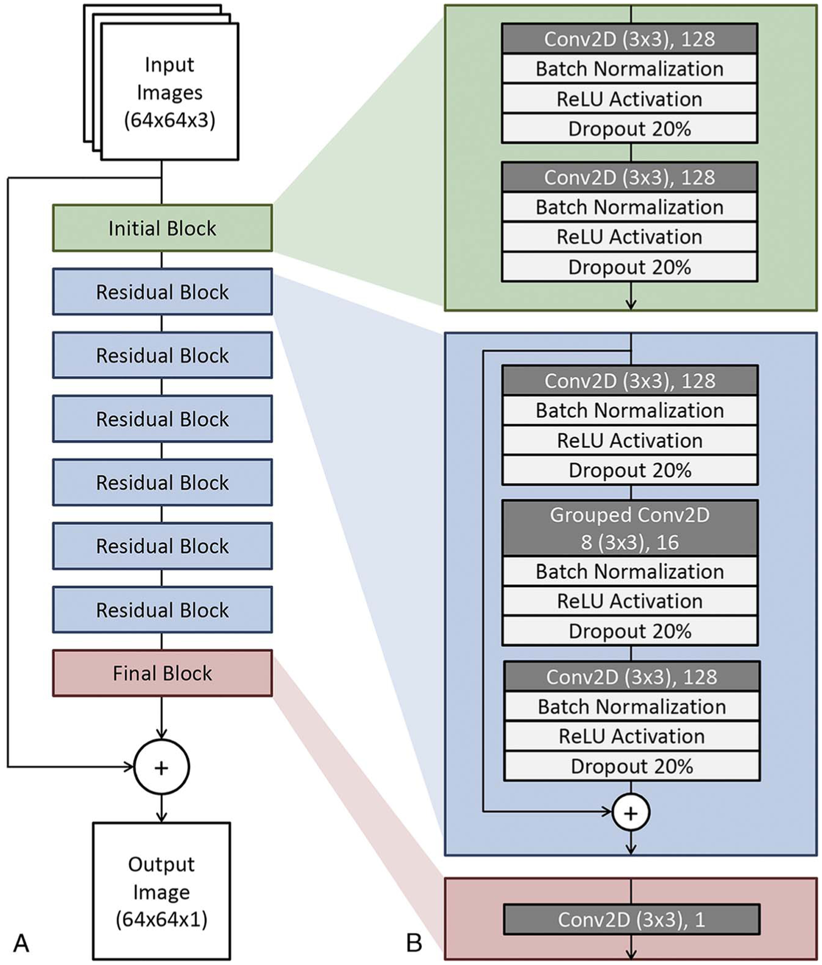
Residual CNN architecture for low-dose CT denoising. A, Block structure of the network containing an initial block, 6 residual blocks, and a final block. Note the additive path from input to just before output in order for the network to learn perturbative noise correction. B, Details regarding the convolutional layers and transformations used within each block. Conv2D indicates 2-dimensional convolutional layer; N, arbitrary image size; ReLU, rectified linear units.

The CNN inputs consisted of 3 adjacent images along the scan direction. The input images were first subjected to initial layers that rescaled the pixel values and generated 128 feature maps using convolutional layers. The feature maps were then operated on by a series of residual blocks. Each residual block consisted of repeated layers of convolutional, batch normalization, rectified linear unit activation, and 20% dropout operations.

A final convolutional layer with linear activation projected the feature maps back into the image domain. The output of the CNN was then subtracted from the central input images. The output could be interpreted as a perturbative correction consisting of the estimated noise textures present in the centermost input image (see Fig. 1). A key feature of this approach compared with others¹³ is the highly residual architecture, which aims to preserve the existing features found in the original input images.

Training and Validation Data Set

We used examinations from the Mayo Clinic/American Association of Physicists in Medicine Low-Dose CT Grand Challenge¹⁶ data set to train the CNN denoising algorithm. This data set consisted of multiple abdominal CT scans (Somatom Definition AS+ or Somatom Definition Flash) performed with routine dose level; we will refer to these examinations as full dose (FD). In addition, a simulated quarter dose (QD) examination was generated for each case using a realistic noise insertion method developed by Yu et al.¹⁷ For training, 250,000 matched QD and FD patches were randomly cropped from reconstructed images in 10 patient examinations. The patch size was 64 × 64 × 3 pixels, with the 3 channels storing 3 adjacent axial images. All training data were reconstructed with a 275-mm FOV, a medium smooth kernel (D30), and 3-mm image thickness.

During training, 3 adjacent QD CT image patches were used as inputs, and the corresponding central image from the FD image patches was used as the CNN target. Batch size was fixed at 20 patches during training. Gradient-based optimization was implemented using Adam optimizer¹⁸ with a descending learning rate from 0.001 to 0.00001. Pixelwise mean squared error between CNN output and FD image was used as the loss function during optimization.

Testing Data Set

Six patient examinations from the Grand Challenge data set were reserved for testing network performance. During testing, the CNN was applied to full reconstructed images with 2 adjacent images along the scan direction (512 × 512 × 3). When evaluating baseline performance, the test set consisted of images that were reconstructed with exactly the same conditions as the training data set. When evaluating the robustness to reconstruction variations, the test set consisted of images reconstructed differently than the training data set. Each variation was applied individually to evaluate the singular impact of the parameter. These variations included modifications to reconstruction FOV, reconstruction kernel, or image thickness. The D-kernel used in this study is a quantitative kernel that does not include edge enhancement.

1. Field of view was varied from 100 to 450 mm (100, 150, 200, 225, 250, 275, 300, 325, 350, 400, and 450 mm);

2. Kernel strength was varied from D10 (very smooth) to D50 (medium-sharp) in increments of 10; and

3. Image thickness was varied from 1 to 5 mm in increments of 1 mm.

Evaluating Network Performance

Network performance was evaluated on the basis of qualitative visual comparisons, spatial resolution, noise level, and similarity calculations between the CNN-denoised QD image and corresponding FD image. Spatial resolution was evaluated using visual assessment, difference images, and line profiles. Difference images were used to identify if anatomical features were subtracted during the process of CNN denoising. Line profiles of selected low-contrast lesions were used for gauging whether resolution was lost after the CNN was applied. Loss of spatial resolution relative to baseline as evidenced by visual assessment, difference image, or line profile was deemed a degradation of network performance. Noise level was measured using the standard deviation of CT numbers inside the aorta, which is a largely uniform region of interest. Noise level of CNN-denoised images relative to QD was plotted as a function of each reconstruction variable. Using the FD reference image, the root mean square error (RMSE), peak signal-to-noise ratio (PSNR), and structural similarity (SSIM) were calculated for the CNN-denoised QD image. The RMSE is a measure of error relative to a target image, PSNR is a decibel ratio of signal power to noise power in the image, and SSIM measures perceptual similarity based on luminance, contrast, and structure.^19,20 The normalized RMSE (RMSE_CNN/RMSE_QD) was also plotted as a function of each reconstruction variable. Percent noise reduction was calculated as the difference in noise level between the QD examination and CNN output, divided by the QD noise level. One-sided paired t tests were conducted to test for degradation in CNN performance on different reconstruction conditions relative to baseline. A statistically significant increase in noise level or normalized RMSE was deemed a degradation of denoising efficiency.

RESULTS

Baseline Performance Evaluation

For baseline performance evaluation, test cases were reconstructed with the exact same reconstruction parameters used in the training data set. Figure 2 contains axial images of the liver for 3 patients from the testing data set. Difference images from FD to CNN-denoised QD are provided. Within the difference image, there was no evidence of anatomical features being unintentionally removed during CNN denoising. For the 6 patients in the testing data set, CNN-based denoising reduced noise level relative to QD in the aorta by 73% ± 6%.

FIGURE 2.

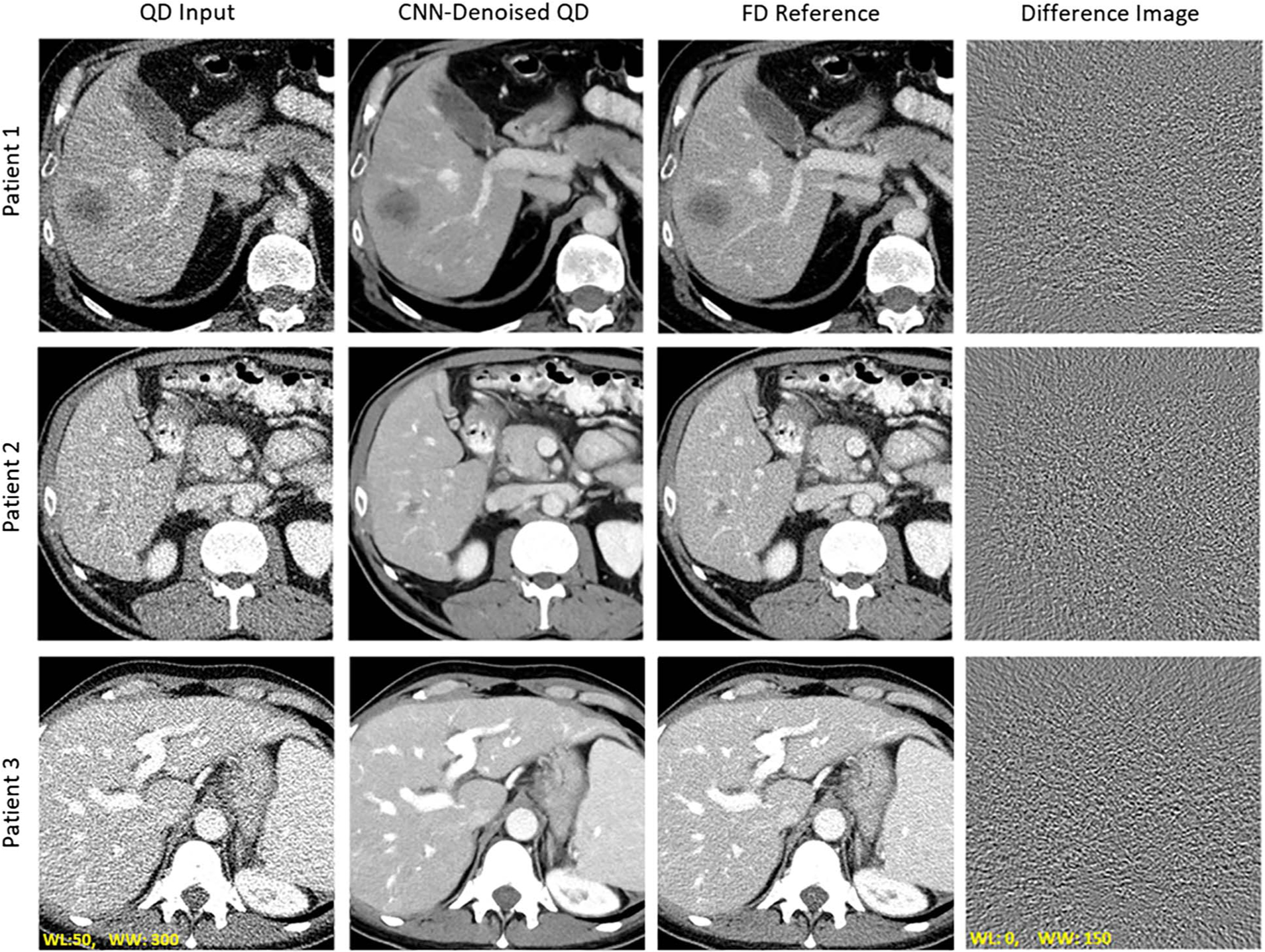
Evaluation of baseline network performance when test data reconstructions match the training data set. Visual examples of CNN denoising performance relative to QD and FD images. The difference image between FD and CNN output was calculated. Note the lack of anatomical details within the difference image.

Performance on Different Reconstruction Conditions

The CNN was trained with images generated from a single reconstruction condition (FOV, 275 mm; kernel, D30; and thickness, 3.0 mm) and applied to various reconstruction conditions. Table 1 provides summary metrics (RMSE, PSNR, and SSIM) for the QD input and CNN output relative to the FD reference.

TABLE 1.

Summary Metrics for a Narrowly Trained CNN Applied to Various Reconstruction Conditions

FOV, mm
	100		200		275		350		450
	QD	CNN	QD	CNN	QD	CNN	QD	CNN	QD	CNN
RMSE, HU	23.3	21.3	20.1	15.9	18.69	11.0	17.1	11.6	14.8	13.6
PSNR, dB	34.5	34.9	38.3	40.2	39.0	43.2	39.8	42.7	41.2	41.2
SSIM	0.89	0.90	0.91	0.95	0.93	0.97	0.94	0.97	0.95	0.97
Reconstruction Kernel
	D10		D20		D30		D40		D50
	QD	CNN	QD	CNN	QD	CNN	QD	CNN	QD	CNN
RMSE, HU	11.2	8.20	14.7	9.82	18.7	11.0	23.3	14.1	51.9	39.1
PSNR, dB	42.9	45.3	40.9	44.0	39.0	43.2	37.3	41.4	30.8	33.7
SSIM	0.97	0.99	0.95	0.98	0.93	0.97	0.90	0.96	0.71	0.83
Image Thickness, mm
	1.0		2.0		3.0		4.0		5.0
	QD	CNN	QD	CNN	QD	CNN	QD	CNN	QD	CNN
RMSE, HU	32.5	18.0	23.0	13.2	18.7	11.0	15.2	9.14	14.7	8.00
PSNR, dB	34.1	39.1	37.0	41.6	39.0	43.2	40.5	44.5	41.2	45.6
SSIM	0.83	0.94	0.90	0.96	0.93	0.97	0.94	0.98	0.94	0.98

Median value for 6 test patients reported. RMSE, PSNR, and SSIM were calculated for 25% dose (QD) and CNN relative to FD reference. The CNN was trained with reconstruction conditions of 275 mm FOV, D30 kernel, and 3 mm image thickness (green highlight).

FOV Varied From 100 to 450 mm

Evaluation with respect to changes in the FOV is shown in Figure 3A. Only 3 FOVs (200, 275, and 350 mm) are shown as examples. When the CNN was applied to the 200 mm FOV, visual impression indicates a decrease in CNN noise reduction efficiency relative to baseline. For the 350 mm FOV case, visual impression suggested a loss of resolution after CNN denoising, which was confirmed with line profiles of a contrast-enhanced vessel in Figure 3B.

FIGURE 3.

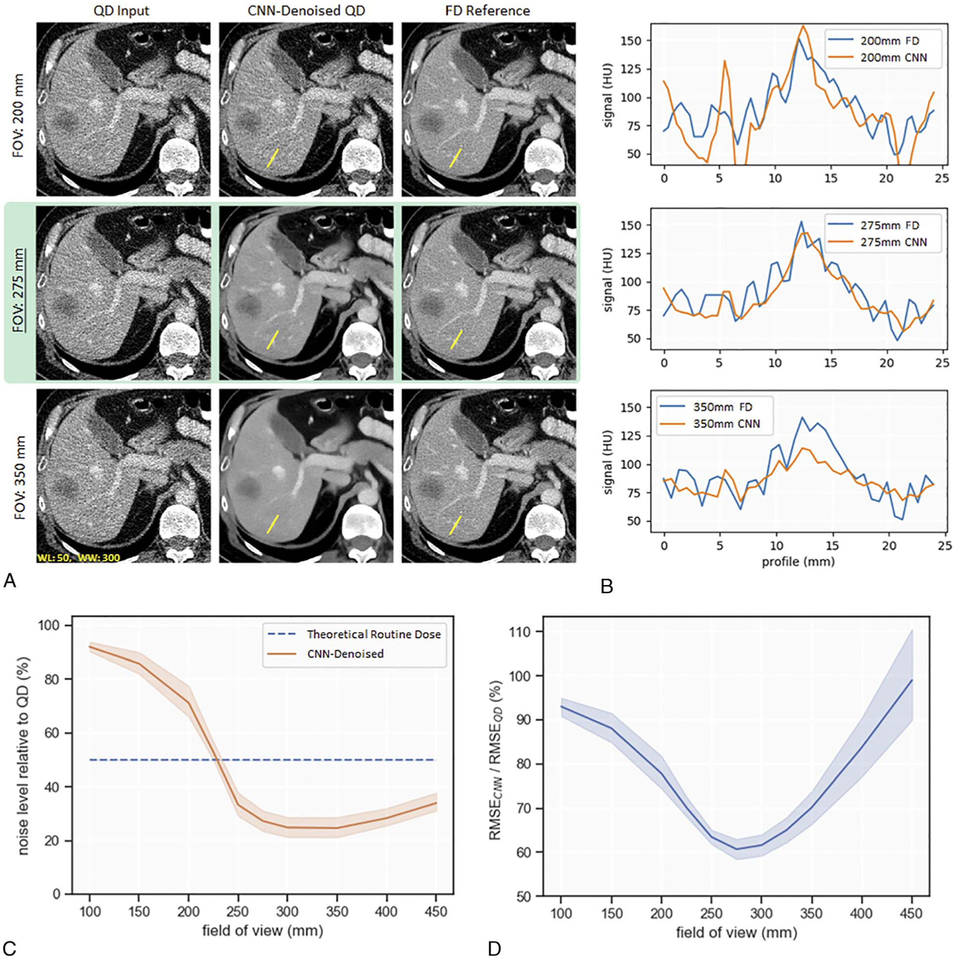
Evaluation of CNN denoising performance to variations in reconstruction FOV. A, Image examples at FOV of 200, 275, and 350 mm, with 275 mm as the baseline (highlighted in green). B, Line profiles of a hypoattenuation lesion within the liver. C, Plot of noise level at the aorta relative to QD. D, Normalized RMSE (RMSE_CNN/RMSE_QD) indicates the pixelwise similarity to the FD images.

Figure 3C depicts a plot of noise level relative to QD for finely sampled alterations in FOV. At baseline, the CNN reduced noise by 73%. There was a statistically significant decrease in amount of noise reduction when the CNN was applied to a decreased FOV, for example, 250 mm of FOV (mean noise reduction of 67%; t[5] = 7.89; P < 0.005). When the CNN was applied to an increased FOV, noise reduction relative to QD remained fairly stable, but visual inspection indicated resolution loss.

Figure 3D depicts a plot of normalized RMSE (RMSE_CNN/RMSE_QD); RMSE_CNN and RMSE_QD were calculated by comparing CNN output and QD to the corresponding FD image. At baseline, the normalized RMSE was 60%. There was a statistically significant increase in normalized RMSE when the CNN was applied to 250 mm of FOV (mean, 63%; t[5] = 4.41; P < 0.005) or 300 mm of FOV (mean, 62%; t[5] = 6.80; P < 0.005). These results suggest an alteration of only ±25 mm FOV from the training set resulted in degradation of this CNN’s denoising performance.

Reconstruction Kernel Varied From D10 to D50

Evaluation with respect to changes in reconstruction kernel is shown in Figure 4A. Only D20, D30, and D40 are shown as examples. Visual impression suggested a reduction in CNN denoising efficacy relative to baseline (D30) when the CNN was applied to D20 kernel images. After CNN denoising of D20 kernel images, artifacts mimicking hepatic lesions were observed within uniform liver regions (Fig. 4A). For the D40 kernel case, visual impression suggested a loss of resolution after CNN denoising. This loss of resolution was confirmed with line profiles of a contrast-enhanced vessel in Figure 4B.

FIGURE 4.

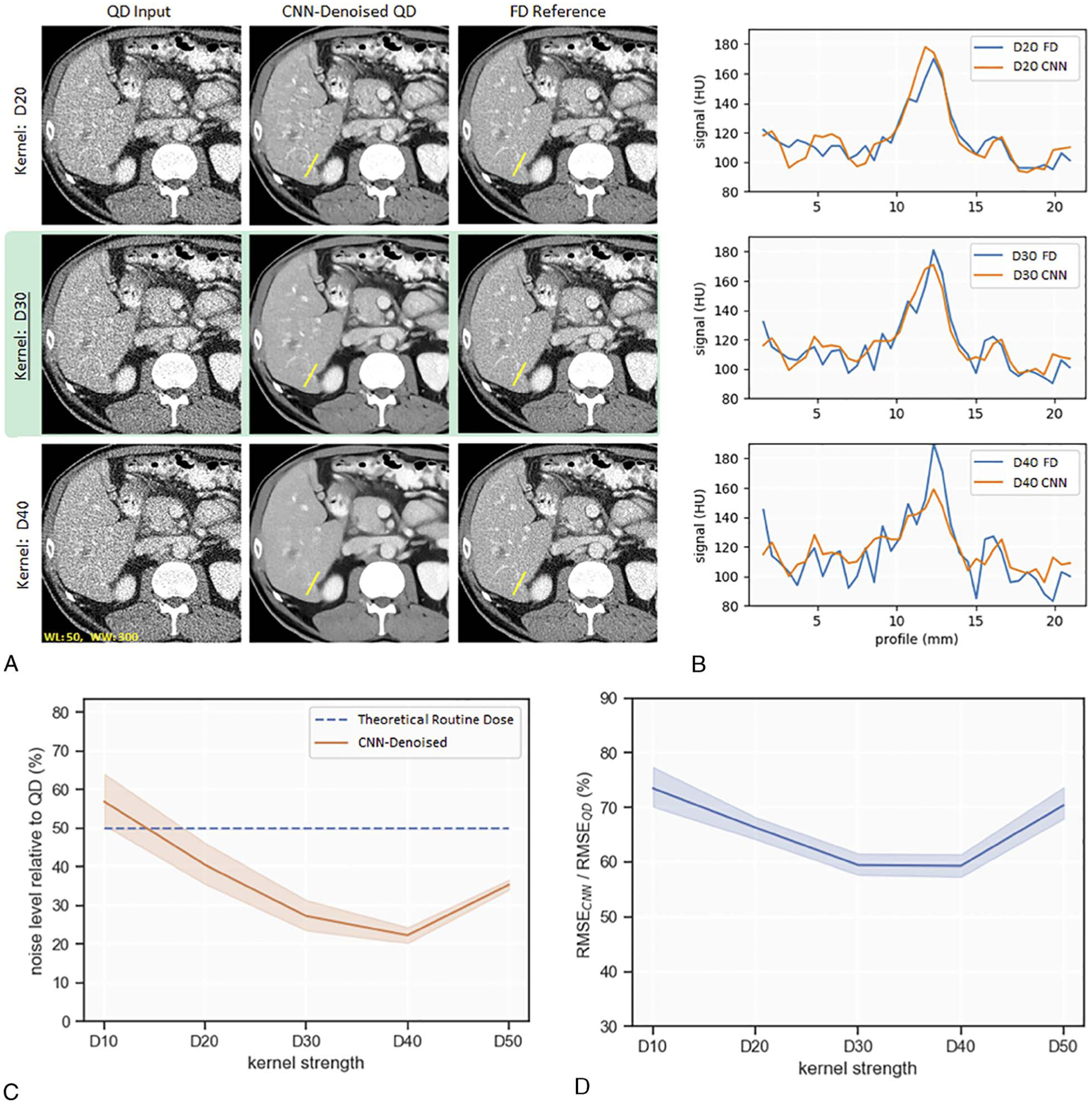
Evaluation of CNN denoising performance to variations in reconstruction kernel. Performance is indicated by visual examples (A), line profiles (B), noise level relative to QD (C), and normalized RMSE (RMSE_CNN/RMSE_QD) (D). D30 is the baseline for comparison (highlighted in green).

Figure 4C is a plot of noise level relative to QD for different kernel strengths. At baseline, the CNN reduced noise in the D30 kernel by 73%. There was a statistically significant decrease in amount of noise reduction when the CNN was applied to a smoother kernel, for example, D20 (mean noise reduction, 60%; t[5] = 7.89; P < 0.005). When the CNN was applied to D40 kernel, percent noise reduction remained constant but visual inspection indicated resolution loss.

At baseline D30 kernel, normalized RMSE (RMSE_CNN/RMSE_QD) was 60%. Figure 4D depicts a statistically significant increase in normalized RMSE for a smoother kernel of D20 (mean, 66%; t[5] = 6.39; P < 0.005) or a sharper kernel of D50 (mean, 70%; t[5] = 12.03; P < 0.005) relative to baseline D30 kernel. These results suggest this CNN’s denoising performance is susceptible to alterations of kernel strength.

Image Thickness Varied From 1 to 5 mm

Evaluation with respect to changes in image thickness is shown in Figure 5A. Visual impression suggested little to no alteration in CNN denoising efficacy relative to baseline when the CNN was applied to 1 mm or 5 mm image thicknesses. Similarly, visual impression suggested resolution after CNN denoising was largely maintained. In Figure 5B, line profile analysis confirmed resolution was maintained at 5 mm image thickness. However, line profiles for the 1 mm image thickness case suggested loss of spatial resolution.

FIGURE 5.

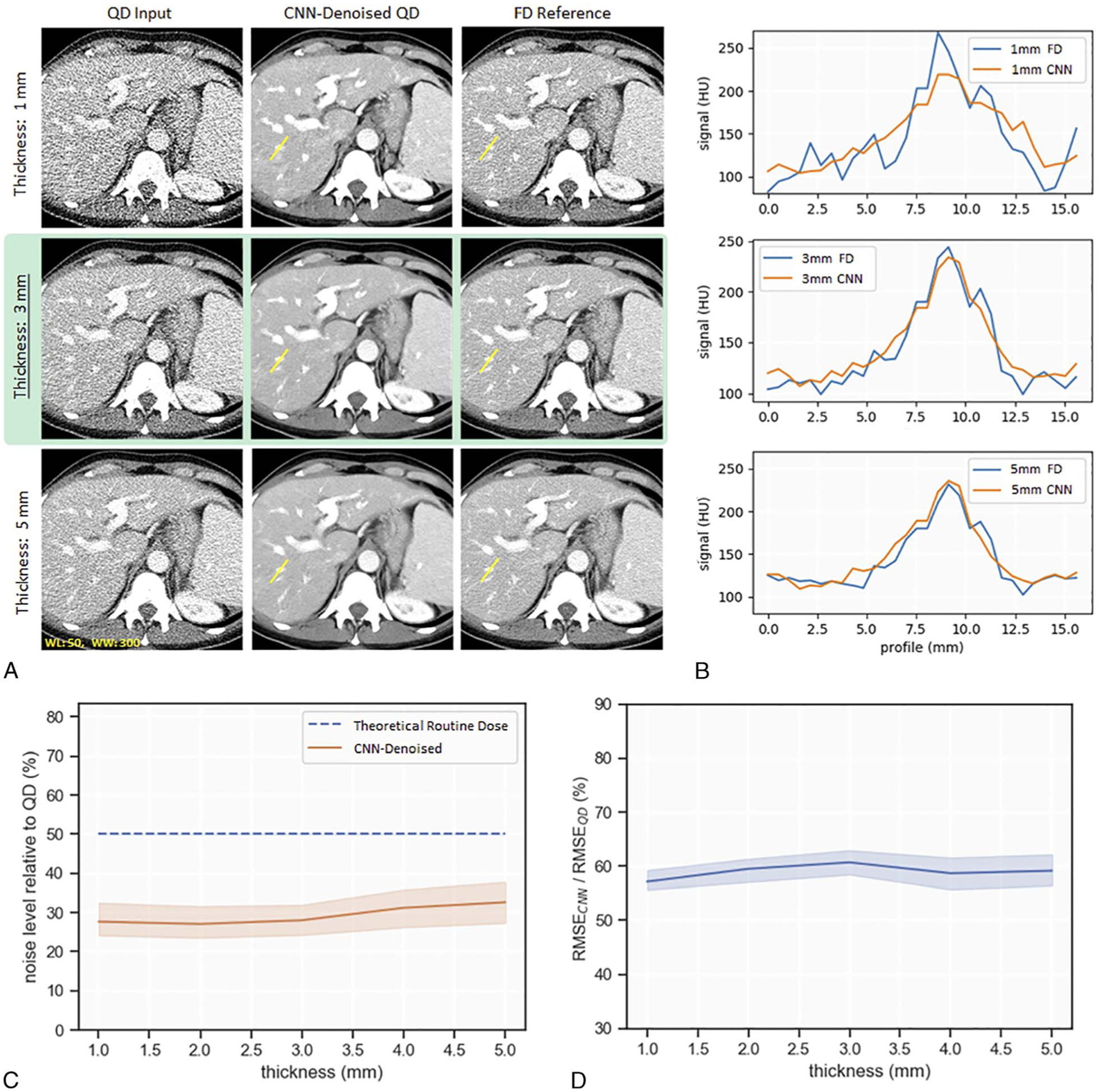
Evaluation of CNN denoising performance to variations in image thickness. Performance is indicated by visual examples (A), line profiles (B), noise level relative to QD (C), and normalized RMSE (RMSE_CNN/RMSE_QD) (D). Image thickness of 3 mm is the baseline for comparison (highlighted in green).

Figure 5C is a plot of noise level relative to QD as a function of input image thickness. There was no significant difference in denoising efficacy for any of the image thicknesses tested. Figure 5D depicts a plot of normalized RMSE (RMSE_CNN/RMSE_QD) for each of the tested slice thicknesses. There was no significant difference in normalized RMSE when slice thickness was altered. These results suggest the CNN’s denoising performance is not degraded by increases in image thickness; however, resolution loss was observed when the CNN was applied to a reduced image thickness of 1 mm.

DISCUSSION

In this study, we explored how the performance of a narrowly trained CNN noise reduction algorithm varies when applied to CT images reconstructed with parameters that differ from those used for the training images. Although some amount of degradation is expected when applying the denoising CNN to images outside of the training scope, the sensitivity to different reconstruction conditions is remarkable. Routine clinical variations in reconstruction FOVand kernel settings are sufficient to introduce measureable and visually obvious deficiencies in denoising performance.

Reconstruction conditions that alter the spatial scales of CT noise textures at the pixel level (eg, reconstruction kernel, FOV) have a larger impact than conditions that primarily alter the overall noise levels (eg, image thickness). Specifically, an observed trend was that when the pixel frequency of noise texture was decreased (eg, decreased FOV), less noise was subtracted by the CNN. On the other hand, if the pixel frequency of the noise texture was higher than that of the training data (eg, sharper kernel), more anatomic features were interpreted as noise by the CNN and subtracted from the input images, resulting in loss of detail and resolution for small anatomic features.

These results have important implications when considering translation of CNN denoising into clinical practice. Some of the reconstruction alterations from training data (smoother kernel and decreased FOV) led to reduced efficiency of the denoising algorithm. Perhaps more concerning, multiple reconstruction alterations (sharper kernel, increased FOV, decreased image thickness) led to a loss of resolution. In clinical tasks, loss of resolution could easily lead to missing critical structure and making incorrect diagnostic conclusions. These results highlight the potential fragility of CNN-based denoising methods when a mismatch exists between the training images and a particular-use case. To anticipate these potential mismatches, an understanding of the images used to optimize the CNN is critical. This work demonstrates the need for transparency when deploying CNN-based denoising algorithms into clinical practice.

In current clinical practice, there are many adjustments in FOV and kernel selection due to patient size differences and task-specific resolution requirements; limiting the clinical reconstruction parameter space to match the training conditions of a CNN denoising algorithm is not a practical option. Instead, many possibilities exist for improving the robustness of the CNN to these clinical variations, such as a more diverse training data set, data augmentation, and different optimized weights, which are used dynamically depending on the input conditions. This work highlights the need for future research along this direction.

There were limitations within this study that should be considered. First, we only explored the “worst-case” scenario where a CNN trained on only 1 specific reconstruction condition is applied to other conditions. The extent to which the robustness of the CNN denoising can be improved is warranted for future studies. Standard image quality metrics must be interpreted with caution when applied to nonlinear CNN denoising networks. Both resolution and noise level after CNN denoising can be dependent on feature contrast, size, and absolute signal level. Task-specific evaluation using either human observers or mathematical model observers for CNN-based denoising remains to be done.^21–24 Finally, CNN denoising robustness was only evaluated for our specific residual network architecture; other architectures may behave differently.

In conclusion, CNN denoising performance is sensitive to minute test set aberrations in FOV and reconstruction kernel relative to training data, with changes to the pixel scale of the noise texture being the most important. When applied to incorrect reconstruction conditions, the CNN output image quality was commonly degraded in terms of resolution loss, image artifacts, or alterations to noise texture.

REFERENCES

- 1.McCollough CH, Primak AN, Braun N, et al. Strategies for reducing radiation dose in CT. Radiol Clin North Am. 2009;47:27–40. [DOI] [PMC free article] [PubMed] [Google Scholar]
- 2.Newman B, Callahan MJ. ALARA (as low as reasonably achievable) CT 2011—executive summary. Pediatr Radiol. 2011;41:453–455. [DOI] [PubMed] [Google Scholar]
- 3.Fletcher JG, Fidler JL, Venkatesh SK, et al. Observer performance with varying radiation dose and reconstruction methods for detection of hepatic metastases. Radiology. 2018;289:455–464. [DOI] [PMC free article] [PubMed] [Google Scholar]
- 4.Hara AK, Paden RG, Silva AC, et al. Iterative reconstruction technique for reducing body radiation dose at CT: feasibility study. AJR Am J Roentgenol. 2009;193:764–771. [DOI] [PubMed] [Google Scholar]
- 5.Wang J, Li T, Lu H, et al. Penalized weighted least-squares approach to sinogram noise reduction and image reconstruction for low-dose x-ray computed tomography. IEEE Trans Med Imaging. 2006;25:1272–1283. [DOI] [PMC free article] [PubMed] [Google Scholar]
- 6.Borsdorf A, Raupach R, Flohr T, et al. Wavelet based noise reduction in CT-images using correlation analysis. IEEE Trans Med Imaging. 2008;27: 1685–1703. [DOI] [PubMed] [Google Scholar]
- 7.Chen Y, Yang Z, Hu Y, et al. Thoracic low-dose CT image processing using an artifact suppressed large-scale nonlocal means. Phys Med Biol. 2012;57: 2667–2688. [DOI] [PubMed] [Google Scholar]
- 8.Li Z, Yu L, Trzasko JD, et al. Adaptive nonlocal means filtering based on local noise level for CT denoising. Med Phys. 2014;41:011908. [DOI] [PubMed] [Google Scholar]
- 9.Rabbani H, Nezafat R, Gazor S. Wavelet-domain medical image denoising using bivariate laplacian mixture model. IEEE Trans Biomed Eng. 2009;56: 2826–2837. [DOI] [PubMed] [Google Scholar]
- 10.Jain V, Seung S. Natural image denoising with convolutional networks. In: Koller D, Schuurmans D, Bengio Y, et al. , eds. Advances in Neural Information Processing Systems 21 (NIPS 2008). Vancouver, Canada; 2008. Available at: https://papers.nips.cc/paper/3506-natural-image-denoising-with-convolutional-networks.pdf.AccessedApril 11, 2019. [Google Scholar]
- 11.Mao X, Shen C, Yang Y. Image restoration using very deep convolutional encoder-decoder networks with symmetric skip connections. In: Lee DD, Sugiyama M, Luxburg UV, et al. , eds. 30th Conference on Neural Information Processing Systems (NIPS). Barcelona, Spain: Cornell University; 2016. Available at: http://arxiv.org/abs/1606.08921.AccessedApril 11, 2019. [Google Scholar]
- 12.Xie J, Xu L, Chen E. Image denoising and inpainting with deep neural networks. In: Pereira F, Burges CJC, Bottou L, et al. , eds. Neural Information Processing Systems Conference. Lake Tahoe, NV; 2012: 350–352. Available at: https://papers.nips.cc/paper/4686-image-denoisingand-inpainting-with-deep-neural-networks.pdf.AccessedApril 11, 2019. [Google Scholar]
- 13.Chen H, Zhang Y, Kalra MK, et al. Low-dose CTwith a residual encoder-decoder convolutional neural network. IEEE Trans Med Imaging. 2017;36:2524–2535. [DOI] [PMC free article] [PubMed] [Google Scholar]
- 14.He K, Zhang X, Ren S, et al. Deep Residual Learning for Image Recognition. Cornell University; 2015. Available at: https://arxiv.org/abs/1512.03385.AccessedJuly 10, 2019. [Google Scholar]
- 15.Xie S, Girshick R, Dollar P, et al. Aggregated Residual Transformations for Deep Neural Networks. Cornell University; 2017. Available at: https://arxiv.org/abs/1611.05431.AccessedJuly 10, 2019. [Google Scholar]
- 16.McCollough CH, Bartley AC, Carter RE, et al. Low-dose CT for the detection and classification of metastatic liver lesions: results of the 2016 low dose CT grand challenge. Med Phys. 2017;44:e339–e352. [DOI] [PMC free article] [PubMed] [Google Scholar]
- 17.Yu L, Shiung M, Jondal D, et al. Development and validation of a practical lower-dose-simulation tool for optimizing computed tomography scan protocols. J Comput Assist Tomogr. 2012;36:477–487. [DOI] [PubMed] [Google Scholar]
- 18.Kingma DP, Ba J. Adam: A Method for Stochastic Optimization. Cornell Univrsity; 2017. Available at: https://arxiv.org/abs/1412.6980.AccessedMay 1, 2020. [Google Scholar]
- 19.Sara U, Akter M, Uddin MS. Image quality assessment through FSIM, SSIM, MSE and PSNR—a comparative study. J Comput Commun. 2019;7: 8–18. [Google Scholar]
- 20.Wang Z, Bovik AC, Sheikh HR, et al. Image quality assessment: from error visibility to structural similarity. IEEE Trans Image Process. 2004;13: 600–612. [DOI] [PubMed] [Google Scholar]
- 21.Fletcher JG, Yu L, Fidler JL, et al. Estimation of observer performance for reduced radiation dose levels in CT: eliminating reduced dose levels that are too low is the first step. Acad Radiol. 2017;24:876–890. [DOI] [PMC free article] [PubMed] [Google Scholar]
- 22.Gong H, Walther A, Hu Q, et al. Correlation between a deep-learning-based model observer and human observer for a realistic lung nodule localization task in chest CT. SPIE Medical Imaging: SPIE. 2019. Available at: 10.1117/12.2513451.AccessedMay 1, 2020. [DOI] [Google Scholar]
- 23.Leng S, Yu L, Zhang Y, et al. Correlation between model observer and human observer performance in CT imaging when lesion location is uncertain. Med Phys. 2013;40:081908. [DOI] [PMC free article] [PubMed] [Google Scholar]
- 24.Zhang Y, Leng S, Yu L, et al. Correlation between human and model observer performance for discrimination task in CT. Phys Med Biol. 2014; 59:3389–3404. [DOI] [PMC free article] [PubMed] [Google Scholar]