Clarifying causal mediation analysis for the applied researcher: Defining effects based on what we want to learn

Abstract

The incorporation of causal inference in mediation analysis has led to theoretical and methodological advancements – effect definitions with causal interpretation, clarification of assumptions required for effect identification, and an expanding array of options for effect estimation. However, the literature on these results is fast-growing and complex, which may be confusing to researchers unfamiliar with causal inference or unfamiliar with mediation. The goal of this paper is to help ease the understanding and adoption of causal mediation analysis. It starts by highlighting a key difference between the causal inference and traditional approaches to mediation analysis and making a case for the need for explicit causal thinking and the causal inference approach in mediation analysis. It then explains in as-plain-as-possible language existing effect types, paying special attention to motivating these effects with different types of research questions, and using concrete examples for illustration. This presentation differentiates two perspectives (or purposes of analysis): the explanatory perspective (aiming to explain the total effect) and the interventional perspective (asking questions about hypothetical interventions on the exposure and mediator, or hypothetically modified exposures). For the latter perspective, the paper proposes tapping into a general class of interventional effects that contains as special cases most of the usual effect types – interventional direct and indirect effects, controlled direct effects and also a generalized interventional direct effect type, as well as the total effect and overall effect. This general class allows flexible effect definitions which better match many research questions than the standard interventional direct and indirect effects.

Mediation analysis is becoming more popular. Fig. 1 shows that both the number of entries in Google Scholar and the number of peer-reviewed articles in PsycINFO that have “mediation analysis” in the title or text have been growing exponentially. While researchers may have long been interested in causal processes, mediation analysis has become more accessible after several decades of accumulation of theory, methods and computing tools. In addition, the investigation of mediators (mechanisms) of intervention effects is now encouraged, or even required, by some research funding agencies, e.g., the National Institute of Mental Health (NIH, 2016). With these push and pull forces, the increased interest in mediation analysis will likely continue, and mediation analyses may exert increasing influence on policy and practice.

Figure 1.

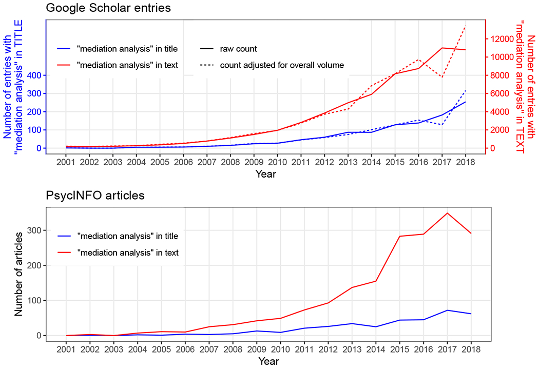
An increasing trend in the popularity of mediation analysis in scholarly research

The raw counts in the top panel are counts reported by Google Scholar on two searches for articles (excluding patents and citations) with “mediation analysis” in the title, and for those with the same phrase anywhere in the text; the adjusted counts are adjusted for the fact that the volume of all Google Scholar entries varies in size from year to year, using 2015 as the standard year. In the bottom panel, the counts are reported by PsycINFO on the same two searches. These searches were conducted on 20/12/2018.

Mediation analysis is not new – the idea dates back to at least as early as Wright (1934), and the seminal Baron and Kenny (1986) paper that popularized mediation analysis in the social sciences was published more than 30 years ago. Yet the methods of mediation analysis are still an active area of research. A major advancement in more recent years is the incorporation of the causal inference approach. This has led to (1) formulation of effect definitions that are more general than those from the prior mainstream (hereafter traditional) approach and that have causal interpretations, and (2) clarification of the assumptions required for such effects to be identified from data, allowing researchers to scrutinize these assumptions based on substantive knowledge; and has opened up (3) a range of relevant estimation methods. However, the methodological literature on causal mediation analysis is fast-growing and complex, which may be confusing to applied researchers and methodologists alike – both those unfamiliar with causal inference and those familiar with causal inference but not specifically with mediation.

Our goal with this paper is to help ease the understanding and adoption of causal mediation analysis. To start, the paper highlights a key distinction between the causal inference and traditional approaches to mediation analysis, and makes a case for explicit causal thinking and the causal inference approach. The bulk of the paper then focuses on the first order of business in causal mediation analysis, defining the target causal effect(s). This first step is important because the effect(s) targeted by an analysis should reflect the research question (what the researchers want to learn), and clarity about this helps the researchers appropriately communicate the results of the analysis (what they have learned). We explain, in one place and in as-plain-as-possible language, several existing effect types: controlled direct effects, natural direct and indirect effects (Robins & Greenland, 1992; Pearl, 2001), and interventional direct and indirect effects (Didelez, Dawid, & Geneletti, 2006; Lok, 2016; Vander-Weele, Vansteelandt, & Robins, 2014). Using concrete examples, we illustrate the types of research questions these effects are fit to answer. This discussion differentiates two general perspectives (or purposes of analysis): the explanatory perspective, aiming to explain the total causal effect; and the interventional perspective, asking questions about hypothetical interventions on the exposure and mediator, or hypothetically modified exposures. We also argue that, if adopting the latter perspective, in many cases we should tap into a more general class of interventional effects rather than restricting to the standard interventional direct and indirect effects.

The key difference between the causal inference and traditional approaches

A typical mediation analysis seeks to understand whether, and to what degree, the effect of an exposure A on an outcome Y involves changing an intermediate variable M. How should such an analysis be done? The answer depends on what is meant by the effect of A on Y through M (the indirect effect). This differs between the two approaches.

The traditional approach uses a model-based definition. It assumes two parametric models: (1) a model for the mediator M with A and covariates C as predictors; and (2) a model for the outcome Y with A, M, C as predictors.^1,2 The indirect effect is defined as the product of the coefficient of A in the mediator model and the coefficient of M in the outcome model. The idea is that these coefficients represent the effect of A on M and the effect of M on Y, so their combination should represent the effect of A on Y through M. The direct effect is defined to be the coefficient of A in the outcome model.³ A triangle diagram is often used to depict these effect definitions (Baron and Kenny, 1986, page 1176; MacKinnon, 2008, page 49; Hayes, 2018, page 83), which we show in Fig. 2 with a small modification to represent covariates. The key point is, the indirect and direct effects here are mathematical objects that do not exist without the model; there is no separation of the definition of an effect and its estimation method.

Figure 2.

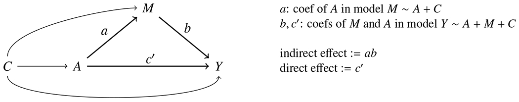
Traditional approach: effects defined as (functions of) regression coefficients

In contrast, the causal inference approach separates the definition of an effect that we researchers want to estimate from how we may estimate it.⁴ Effects are defined in a model-free manner, based on reasoning about what fits the notion of a causal effect. A helpful and popular framework for this purpose is the potential outcomes (aka counterfactual) framework (Splawa-Neyman, 1923; Rubin, 1974; Holland, 1986), in which a causal effect is defined as a contrast between potential outcomes under two different conditions, for the same individual, or the same group. The total effect for an individual (or for a group) is often defined as the difference between (i) the outcome the individual would have (or the average outcome the group would have) if exposed to an exposure of interest and (ii) the outcome the same individual would have (or the average outcome the same group would have) if unexposed. The total effect is thus a contrast of two conditions defined by values of the exposure. Robins and Greenland (1992) and Pearl (2001) extended this reasoning to define an indirect (or a direct) effect as a contrast of two conditions defined by values of the exposure-mediator combination. How these conditions are formulated determines the type of direct and indirect (hereafter “(in)direct”) effects; there are several types of these effects. The first task for a researcher is to determine which effects best match their research question.

After effect definition, the next step in the causal inference approach is effect identification, that is, determining whether the causal effect of interest can be learned from data (aka, is identified). Methodologists have worked out the assumptions required for identification of each effect type; the task of the substantive researcher is to judge whether such assumptions are plausible with their own data. Identification gives us the license to then estimate the causal effect, and it is only at this effect estimation step that modeling questions (e.g., whether to fit a linear model for the mediator and a logistic model for the outcome, or do something else) come into the picture. This separation of the three steps – effect definition, identification, and estimation – is different from the traditional approach.

The need for explicit causal thinking in mediation analysis

We argue that the practice of mediation analysis would benefit from adopting explicit causal thinking. First, mediation analysis is, unavoidably, about causal effects. This is not the case with regular regression analysis, where the target may be either causal effects or conditional associations. In mediation analysis, the arrows drawn from A to M and Y and from M to Y imply a conception that these variables affect one another in the directions depicted. The influence of A on Y through M and the influence of A on Y through other ways – referred to in the research question – are causal effects. Therefore, a mediation analysis, whether using a traditional or causal inference method, is an analysis of causal effects. In addition, results of mediation analysis are generally interpreted in causal terms – regardless of any caution the authors may put in the limitations section. Hence analysis should be done in a way that aims to justify such interpretation. Note that this point, that mediation is conceptually causal, has been made repeatedly by prominent scholars in mediation methodology (e.g., Baron & Kenny, 1986; MacKinnon, 2008; Preacher, 2015).

Second, while mediation analysis is about causal effects, such effects are not intuitively obvious in the mediation setting. In the non-mediation setting, intuition serves us researchers well in the pursuit of causal effects. For example, suppose we are interested in the effectiveness of a short-term college preparation program as an intervention to improve college readiness in high school students. If a trial randomizes high-schoolers to receive either this intervention or no intervention, and subsequently measures their readiness for college, it is rather obvious that the difference in college readiness between the students who received and those who did not receive the intervention represents the effect of the intervention. We may make this comparison and attribution intuitively, without consciously considering why. The implicit reasoning here, were we asked to explain ourselves, is that we observe the outcome in both of the conditions (intervention and no intervention) we wish to compare, and the two groups in the two conditions are similar (due to randomization) so it is reasonable to simply compare their outcomes. In the mediation setting, on the other hand, for a direct (or indirect) effect, we no longer have two observable conditions to compare. Suppose we wish to know the effect of this intervention that is mediated by an intermediate variable, self-awareness. Extending the reasoning above, we might wish, for example, to compare college readiness in two conditions: (a) the intervention condition and (b) a (hypothetically) modified intervention condition where the intervention is forced not to influence self-awareness (thus the intervention’s effect on college readiness through self-awareness is blocked); this difference would be a fine notion of an indirect effect.⁵ However, condition (b) does not exist, thus cannot be observed. The challenge of the mediation setting is that we do not have observable contrasts that correspond to lay perceptions of causal effects. Here, adopting explicit causal thinking allows us to be more clear about what exactly are the causal effects we want to learn (the focus of the later part of this paper), and to figure out whether, and how, we can learn it.

But there lingers the question: What is the problem with simply using the product of coefficients, which seems so intuitive? A brief answer: In the simplest case where linear models are used, for the product of coefficients to match a causal indirect effect (in the sense of the outcome contrast between conditions (a) and (b) in the example above), the following conditions are generally required: (1) all identification assumptions hold (roughly speaking, covariates C are pre-exposure and capture all A-M, A-Y and M-Y confounding); (2) the additive effect of M on Y does not depend on the value of A (aka no A-M interaction) or on the base value of M (aka Y is linear in M); (3) either the additive effect of A on M or the additive effect of M on Y is the same across all individuals, or these two effects are independent of each other (aka constant or independent additive effects); and (4) the correct forms of C are used in both models and do not interact with A and M. (Similar assumptions are discussed in MacKinnon, 2008, chapter 3.) These are strong assumptions. The fourth one may be relaxed to some extent, e.g., when evaluating conditional effects within levels of C, but not the other three. The no A-M interaction assumption is overly restrictive, as there are cases where such an interaction is expected (MacKinnon, Valente, & Gonzalez, 2019). If nonlinear models are used, the product of coefficients generally does not match, and may not be on the same scale as, the causal effect of interest.

Technical details aside, a general point is that as model assumptions are unlikely to hold, one may want to minimize them, or at least have flexibility in their selection; thus it makes sense to define effects in a model-free manner to have clarity about what we are trying to learn and avoid having a moving target. The causal inference approach fits this bill. To be clear, adopting the causal inference approach generally does not remove the need for some model assumptions at the estimation step. But instead of defaulting to a set of models, with model-free effect definitions we can consider what models to use based on the data at hand and based on what prior knowledge we have or do not have about the causal structure. Such consideration likely results in adopting more flexible models that make fewer assumptions,⁶ or assumptions that are more appropriate to the specific situation.

To mediation analysis, causal inference is a new approach, and it takes time for new approaches to take hold. A certain degree of interest in the causal inference perspective is seen in recent works by several methodologists known for substantial contribution in the traditional approach – these works include causal inference as a topic in mediation analysis methodological reviews (Mackinnon, Fairchild, & Fritz, 2007; MacKinnon, Kisbu-Sakarya, & Gottschall, 2013), emphasize confounding as a validity threat in mediation analysis (MacKinnon et al., 2013; MacKinnon & Pirlott, 2015), highlight the need to accommodate exposure-mediator interaction (MacKinnon et al., 2019), and explain how to implement causal mediation analysis (Miočević, Gonzalez, Valente, & MacKinnon, 2018; Muthén, 2011; Muthén & Asparouhov, 2015). In the applied research literature, however, the uptake of causal mediation analysis is still limited. In an ongoing review of articles published in top psychology and psychiatry journals in 2013-2018 that include a mediation analysis, we found that less than 4% used causal mediation analysis. In our experience working with researchers (students, postdocs and faculty) in a public health research institution, we observe that often the researcher’s less than ideal starting point (e.g., unfamiliarity with causal inference language, or loose understanding of confounding and confounding control) combined with the complexity of the methodology (e.g., multiple effect definitions and identification assumptions, different settings requiring different methods, and the explosion of the methodological literature) hinders adoption of causal mediation analysis. We aim to help address these barriers, starting with the current paper.

Orientation to the rest of the paper

Before delving into the causal effects, it is important to point out that this paper does not address analyses in the research literature which are unfortunately also referred to as mediation analyses, but do not reflect a setting where it is plausible for A to influence M and Y and/or for M to influence Y, for example due to lack of temporal ordering of these variables. These are analyses of associations (not causal effects), and in our opinion it is more appropriate to refer to them as “third variable analyses”. Third variable analyses require a separate discussion that is outside the scope of the current paper.

Another third variable setting not covered here is where there is temporal ordering but the intermediate variable of interest is defined based on only one exposure condition (e.g., adherence to the active treatment or attendance of intervention sessions). For this problem a principal stratification (Frangakis & Rubin, 2002) approach could be used – see Imai, Jo, and Stuart (2011); Jo and Stuart (2009, 2012); Jo, Stuart, Mackinnon, and Vinokur (2011); note that causal effects defined in this approach are different from those discussed in the current paper. In our current mediation analysis setting, the mediator is a variable that is defined and has the same meaning for both exposure conditions; the key idea is the exposure (relative to nonexposure) makes a difference in the mediator, and that results in an effect on the outcome.

Back to the task at hand, of the three steps in causal mediation analysis, the remainder of this paper focuses on the first step – effect definition. We start with the total effect, showing how it is defined based on potential outcomes at the individual and population levels, laying down basic causal inference concepts. We also introduce the causal directed acyclic graph (DAG), a helpful tool for visualizing effect definitions and assumptions. We then bring in the mediator, and define, and discuss the practical relevance of, several effect types, first the natural (in)direct effects, then the interventional (in)direct effects, then a broader class of interventional effects, and ending with controlled direct effects.

This somewhat unusual order of presenting these effect types – e.g., controlled direct effects not appearing first and not preceding natural (in)direct effects as in most papers that include both these effect types – results from our attention to having the effects motivated by questions of potential practical relevance. This ordering of the effects reflects a reasonable ordering of the sorts of questions they answer. While following this line of thinking, we stumbled upon the broad class of interventional effects. This class includes, in addition to the interventional (in)direct effects, several other effect variations that are more intuitive and fit certain research questions better than the interventional (in)direct effects.

As the focus is on effect definition, we mostly put aside questions about whether an effect is identified and how it may be estimated, except a couple of identification comments called for by the juxtaposition of interventional and natural (in)direct effect types. The closing remarks provide brief comments that aim to orient the reader to these two topics, and refer the reader to the relevant literature.

This paper does not assume that the reader is well versed in causal inference reasoning. We use as plain as possible language combined with examples to elucidate concepts and ideas. While some mathematical notation is needed, it is accompanied by explanations in English and is color-coded for easy recognition. Also, the paper includes extensive footnotes. We recommend that the reader skip the footnotes on the first read of the paper, and come back to them on a second read. The footnotes are not required for understanding the main content, but provide additional explanations to deepen understanding, and expose a broader range of terms and concepts encountered in the causal mediation literature, which may help the reader be an effective consumer of that literature.

For simple presentation, we use the situation with a binary exposure, one mediator and one outcome. The content here applies directly to a non-binary exposure (replacing the exposed and unexposed conditions with the contrast of A = a and A = a* where a is the exposure level of interest and a* is the comparison level), multiple outcomes (treated as one outcome vector), and multiple mediators considered enbloc (as one mediator vector). Solid understanding of this case will make it easier to deal with more complex situations.

Total effect

Again, consider our intervention for high school students (the exposure) and their college readiness (the outcome). Each student (indexed by i) has two potential outcomes, one is the college readiness level that the student would have if exposed to the intervention, the other is the college readiness level they would have if not exposed to the intervention. These are two different variables, labeled Y_i,(1) and Y_i(0), where 1 and 0 stand for the exposed and unexposed conditions. The individual total effect, denoted TE_i, is often defined on the additive scale as the difference between these two potential outcomes,

$$T{E}_i:=Y_i\left(1\right)-Y_i\left(0\right),$$

where the symbol := means “is defined as”. Averaging the individual total effects over the population⁷ of high school students, we have the average total effect, denoted TE,

$$\text{TE}:=\text{E}\left[Y\left(1\right)\right]-\text{E}\left[Y\left(0\right)\right],$$

where E[·] denotes expectation (population mean).⁸ If the outcome is binary (coded 0/1), this definition is equivalent to TE = P(Y(1)=1) – P(Y(0)=1), a risk difference.

To make things concrete, Table 1 shows a toy example where the population consists of eight individuals. For each individual, both potential outcomes (values on a 0-10 scale) and the total effect are shown. TE is an average increase in college readiness of 1.625 points (the average of all the T E_i values in the table). In reality, however, we are not privy to individual effects, for we never observe both potential outcomes for the same individual. What we observe is the realized outcome Y_i, which reveals one of the potential outcomes. Specifically, we observe Y_i = Y_i(1) if the student is exposed to the intervention (A₁ = 1), and Y_i = Y_i(0) if the student is not exposed to the intervention (A_i = 0).⁹ The puzzle for researchers is that given the data in the last two columns of the table, we want to learn about the average total effect, and more.

Table 1.

Individual total effects: a toy example

	Potential outcomes		Total effect	OBSERVED DATA
i	Yi(0)	Yi(1)	TEi = Yi(1) – Yi(0)	A i	Y i
Bo	4	9	5	1	9
Sam	7	8	1	1	8
Ian	5	7	2	1	7
Ben	8	7	−1	1	7
Suri	3	5	2	0	3
Bill	6	7	1	0	6
Kat	9	8	−1	0	9
Dre	4	8	4	0	4

Introducing the causal DAG.

A causal DAG (Pearl, 2009) consists of nodes that represent variables and arrows that represent causal effects; all common causes of any pair of variables are included; and there is no directed path from a variable (through other variables) to itself. Consider the DAG in Fig. 3a which shows the world without any (real or imagined) manipulation by the investigator. The variables of interest are A (college prep program participation) and Y (college readiness). C represents common causes of A and Y – variables that may make a high school student more or less likely to attend a college preparation program and that influence college readiness (e.g., academic achievement, socio-economic status, etc.). Another name for a common cause is confounder, so C consists of confounders of the A-Y relationship. This DAG also shows that A and Y have causes that are not shared, U_A and U_Y (where U stands for unique causes); these may also be left out of the DAG and their presence is implicitly understood.¹⁰

Figure 3.

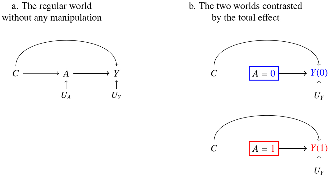
The total effect

The total effect is a contrast between two parallel worlds which we imagine for the same individual (or the same group of individuals). In these two worlds, everything is the same, except that in one world A is set to 1 (program participation, i.e., the exposed condition), and in the other world A is set to 0 (nonparticipation, i.e., the unexposed condition). These are shown in the two DAGs in Fig. 3b, where the box represents that a variable is set to a value. In these two DAGs, since A is set to a fixed value for everyone, this breaks the causal link between C and A.

Natural (in)direct effects

As mentioned earlier, there is more than one (in)direct effect type. To start, consider a common motivation of mediation analysis, the desire to explain the effect of the exposure on the outcome. The question often asked is: How much (if any) of this effect went through the mediator, and how much went through other ways? Natural (in)direct effects (Robins and Greenland, 1992; Pearl, 2001)¹¹ capture the essence of this question.

The definition of these effects starts at the individual level. The idea is to split the individual total effect TE_i – the contrast of Y_i(1) and Y_i(0) – into two contrasts using a third potential outcome that is in-between in some sense, so that one contrast represents a mediated effect, the other a direct effect, for the individual. What should be this third potential outcome? The outcome in a hypothetical world where the exposure is set to one condition, but the mediator is set to its potential value under the other exposure condition. (This world is a product of our imagination that cannot realize or be observed, but is conceptualized in order to help decompose the total effect into meaningful and somewhat interpretable pieces.)

To see how this works, we need to be a bit more formal. Let Y_i(a) denote the potential outcome of individual i if exposure is set to a (where a can be either 1 or 0, so any statement about Y_i(a) applies to both Y_i(1) and Y_i(0)). Similarly, let M_i(a) denote the potential mediator value for individual i if exposure is set to a. Also, consider a new type of potential outcome, Y_i(a, m), the potential outcome when exposure is set to a and mediator is set to m. Depending on the mediator distribution, there may be many such potential outcomes – two for each possible m value. Yet we are not interested in just any m value. For each individual, only two values are relevant: M_i(1) and M_i(0), the values that the mediator would naturally take under the two exposure conditions. This is because the mediated part of TE_i occurs only because the exposure has an effect on the mediator, and that effect is the difference between M_i(1) and M_i(0). Hence we replace m in Y_i(a, m) with one of these values, denoted M_i(a′) (where a′ can also be either 0 or 1), and obtain Y_i(a, M_i(a′)), the potential outcome in a world where the exposure is set to a and the mediator is set to the value it would take under exposure a′.

When a and a′ are the same, we have Y_i(a, M_i(a)), which is equal to Y_i(a). That is, the potential outcome in a world where exposure is set to a and mediator is set to M_i(a) is the same as the potential outcome in a world where exposure is set to a and mediator follows naturally.¹² TE_i is thus a shift from Y_i(0) = Y_i(0, M_i(0)) to Y_i(1) = Y_i(1, M_i(1)).

Our in-between world is one where a and a′ are not the same. One choice is the world where the exposure is set to 1, but the mediator is set, for each individual, to their M_i(0). With this as the in-between world, TE_i is split into two parts: Part 1 is a shift from Y_i(0, M_i(0)) to the in-between potential outcome Y_i(1, M_i(0)). This fits the notion of a direct effect (and is called a natural direct effect (NDE)), as it is the effect of changing the exposure from 0 to 1 but fixing the mediator (not letting the mediator change in response to the exposure change). Part 2 is a shift from Y_i(1, M_i(0)) to Y_i(1, M_i(1)). This fits the notion of an indirect effect (and is called a natural indirect effect (NIE)), as it is the effect of the mediator switching from M_i(0) to M_i(1) (as if in response to a change in exposure), while the exposure is actually fixed (so there is no direct effect element).

For concreteness, consider Bo, one of our high school students. Suppose we are omniscient and know what would happen in all the different worlds. If Bo participated in the college prep program, Bo would have high self-awareness and college readiness level 9 – these are M_Bo(1) and Y_Bo(1). If Bo did not participate in the program, Bo would have low self-awareness and college readiness level 4 – these are M_Bo(0) and Y_Bo(0). The total effect of the intervention for Bo is thus an increase in college readiness of 5 points. In the in-between world where Bo participated in the program but somehow Bo’s self-awareness was fixed at its level under nonparticipation, M_Bo(0) (i.e., low), Bo would attain college readiness level 7 – this is Y_Bo(1, M_Bo(0)). This means the NDE for Bo is an increase in college readiness of 3 points, from level 4 to 7, and the NIE is a further increase of 2 points, from level 7 to 9. Table 2 shows these effects for all the high-schoolers in our toy example.

Table 2.

Individual natural (in)direct effets of the direct-indirect decomposition: a toy example

i	Potential mediators		Potential outcomes			Direct-indirect decomposition		OBSERVED DATA
	Mi(0)	Mi(1)	Yi(0)	Yi(1, Mi(0))	Yi(1)	NDEi(·0)	NIEi(1·)	Ai	Mi	Yi
Bo	low	high	4	7	9	3	2	1	high	9
Sam	medium	high	7	7	8	0	1	1	high	8
Ian	low	low	5	7	7	2	0	1	low	7
Ben	low	medium	8	6	7	−2	1	1	medium	7
Suri	low	high	3	3	5	0	2	0	low	3
Bill	low	medium	6	5	7	−1	2	0	low	6
Kat	high	high	9	8	8	1	0	0	high	9
Dre	medium	high	4	7	8	3	1	0	medium	4

We refer to the above decomposition of the total effect the direct-indirect decomposition, based on the order of the component effects. Alternatively, we can use the other in-between world with Y_i(0, M_i(1)) to split the total effect into a NIE followed by a NDE – the indirect-direct decomposition.

The average natural (in)direct effects, which are population means of the individual effects, decompose the average total effect:

direct-indirect decomposition:

$$\text{TE}=\underset{\text{NIE}\left(1\cdot \right)}{\underbrace{\text{E}\left[Y\left(1,M\left(1\right)\right)\right]-\text{E}\left[Y\left(1,M\left(0\right)\right)\right]}}+\underset{\text{NDE}\left(\cdot 0\right)}{\underbrace{\text{E}\left[Y\left(1,M\left(0\right)\right)\right]-\text{E}\left[Y\left(0,M\left(0\right)\right)\right]}},$$

indirect-direct decomposition:

$$\text{TE}=\underset{\text{NDE}\left(\cdot 1\right)}{\underbrace{\text{E}\left[Y\left(1,M\left(1\right)\right)\right]-\text{E}\left[Y\left(0,M\left(1\right)\right)\right]}}+\underset{\text{NIE}\left(0\cdot \right)}{\underbrace{\text{E}\left[Y\left(0,M\left(1\right)\right)\right]-\text{E}\left[Y\left(0,M\left(0\right)\right)\right]}}.$$

To differentiate between the two NDEs and the two NIEs,¹³ here we index each of these effects with a combination of a dot representing the condition (either exposure or mediator) that varies in the contrast, and a number representing the condition that is fixed.¹⁴

Revisiting the causal DAG.

Fig. 4 shows the direct-indirect decomposition of the total effect. Fig. 4a is the unmanipulated DAG. In Fig. 4b, the top and bottom DAGs represent the two worlds contrasted by the total effect, where the mediator follows naturally after the exposure. The middle DAG in Fig. 4b represents the in-between world, where the mediator is set to its value under the opposite exposure condition.¹⁵

Figure 4.

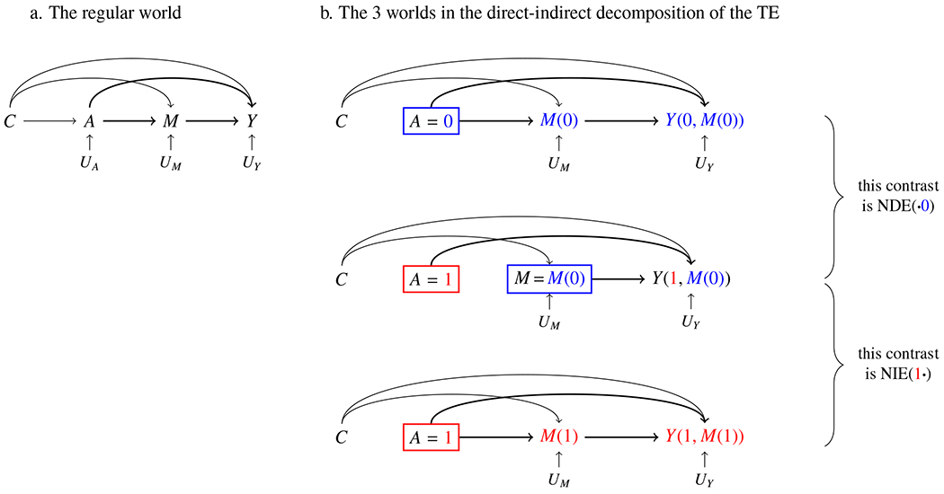
Natural (in)direct effects – depicted in the special case with no intermediate confounder

Note that C in Fig. 4 is different from C in Fig. 3. Here C collectively represents three sets of confounders, of the A-M, A-Y and M-Y relationships, which may overlap but may not be identical. Note also that this figure represents the special (and simple) case where no M-Y confounders are influenced by A. In the general case (see Fig. 5a), in addition to M-Y confounders not influenced by A (included in C), there are M-Y confounders influenced by A (termed intermediate confounders) represented by L.¹⁶

Figure 5.

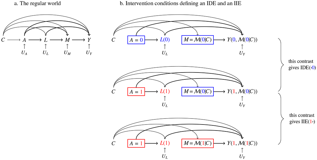
Interventional (in)direct effects – depicted in the general case with an intermediate confounder

Figure note: An equivalent representation of Y(a, $\mathcal{M}$(a′|C)) is Y(a, L(a), $\mathcal{M}$(a′|C)).

In our experience, when first introduced, the natural (in)direct effects may take some time to sink in. We offer two heuristics that might help build intuition for these effects.

Heuristic definition 1: information flows.

Consider a system with three variables, exposure, mediator and outcome; and two paths along which information can flow in the system: the exposure → outcome path, and the exposure → mediator → outcome path. In the default condition of the system, called the unexposed condition,

$$\begin{array}{ccc}\text{exposure}=0,& \text{mediator}=M\left(0\right),& \text{outcome}=Y\left(0,M\left(0\right)\right),\end{array}$$

and there is no information movement. If we switch the exposure from 0 to 1, this change is information. This information flows through both paths, and affects any variable it comes across. This results in a switch of both the mediator and the outcome, obtaining a new condition for the system, called the exposed condition, where

$$\begin{array}{ccc}\text{exposure}=1,& \text{mediator}=M\left(1\right),& \text{outcome}=Y\left(1,M\left(1\right)\right).\end{array}$$

The outcome switch from the unexposed to the exposed condition is the total effect.

Decomposition of the total effect is analogous to staggering the flow of information – by turning a path off and on. Suppose we turn off the exposure → mediator → outcome path. When the exposure is switched from 0 to 1, the generated information can flow only through the exposure → outcome path. It does not reach, therefore does not affect, the mediator. But it reaches the outcome and causes it to change. As a result, the system obtains a mid-way condition, where

$$\begin{array}{ccc}\text{exposure}=1,& \text{mediator}=M\left(0\right),& \text{outcome}=Y\left(1,M\left(0\right)\right).\end{array}$$

Now we turn the exposure → mediator → outcome path back on. Information now flows through this path. It reaches the mediator, causing it to change. This flow of information then reaches the outcome, causing the outcome to change. This takes the system to the exposed condition. The two outcome shifts, from the unexposed to the mid-way condition, and from the mid-way to the exposed condition, are the NDE(·0) and NIE(1·).

If instead of turning off and on the exposure → mediator → outcome path, we turn off and on the exposure → outcome path, then we have an alternative mid-way condition where mediator = M(1) and outcome = Y(0, M(1)). In this case, the two outcome shifts correspond to the NIE(0·) and NDE(·1).

Heuristic definition 2: double exposure.

Another way to think about natural (in)direct effects is to imagine that the exposure A is the combination of two exposures denoted A^M and A^R. A switch of A^M from 0 to 1 causes a switch of the mediator from M(0) to M(1), so A^M is responsible for any influence of A on the outcome through the mediator. A^R is responsible for all the remaining influence of A. We only observe situations where these two exposures go together, A^R = A^M = A = 1 or = 0. But imagine that they do not need to go together. With two exposures, we have potential outcomes of the form Y(a, a′), the outcome that would occur if A^R were set to a and A^M to a′. The total effect previously defined corresponds to the effect of both exposures combined,

$$\text{TE}=\text{E}\left[Y\left(1,1\right)\right]-\text{E}\left[Y\left(0,0\right)\right].$$

Its direct-indirect decomposition is given by adding and subtracting E[Y(1, 0)], i.e.,

$$\text{TE}=\underset{\text{NIE}\left(1\cdot \right)}{\underbrace{\text{E}\left[Y\left(1,1\right)\right]-\text{E}\left[Y\left(1,0\right)\right]}}+\underset{\text{NDE}\left(\cdot 0\right)}{\underbrace{\text{E}\left[Y\left(1,0\right)\right]-\text{E}\left[Y\left(0,0\right)\right]}},$$

and its indirect-direct decomposition is given by adding and subtracting E[Y(0, 1)]. In this representation, the two NDEs are the effects of A^R when A^M is set to 0 and to 1, and the two NIEs are the effects of A^M when A^R is set to 0 and to 1.

Why two decompositions and which one to choose?

As mentioned above, natural (in)direct effects match the purpose of explaining the causal effect, answering the question what part of the total effect went through the mediator and what part did not. These effects have thus been called “descriptive” (Pearl, 2001). A seemingly complicating matter is that with two decompositions of the total effect into natural (in)direct effects, there is not a single NDE or a single NIE. Generally, NIE(1·) and NIE(0·) are not the same, and neither are NDE(·0) and NDE(·1). This is not a weakness of these effects. On the contrary, it reveals an implicit assumption in our original question, that the total effect can be split into two effects that are separate and do not interact – which, in the language of the double exposure heuristic definition, means the effect of A^R must be constant for both levels of A^M and vice versa. This is an arbitrary assumption.

A practical question remains: For a specific analysis, which decomposition should be used? Or should both be used? Our view is that answering this question requires being more clear about the research question/objective. We propose three answers for three cases.

Case 1: Is there a mediated effect? Or, is the causal effect (partly) mediated by this putative mediator? (And if yes, what is the size of the effect?) With this research question, we propose using the direct-indirect decomposition. The rationale is that here we are not questioning the existence of a direct effect, but are considering the possibility of a mediated effect in addition to the direct effect; if there is no mediated effect (either because the mediator does not change in response to the exposure, or it does change but that change does not cause a change in the outcome), then the total effect is the same as NDE(·0), the direct effect in the direct-indirect decomposition.

Case 2: In addition to the mediated effect, is there a direct effect? Or, does the exposure influence the outcome in other ways, not through this mediator? (And if yes, what is the size of this effect?) This is a mirror image of the previous case, just flipping the relative order of direct and indirect effects. We propose using the indirect-direct decomposition. If there is no direct effect, then the total effect is the same as NIE(0·), the indirect effect in the indirect-direct decomposition.

Case 3: The objective is to describe the effect of exposure on outcome with direct and indirect effect elements, without any prior assumption or preferred question about either direct or indirect effects. In this case, we propose presenting both decompositions. After all, if the purpose is simply to describe all we can learn, there is no reason to prefer either decomposition over the other.

While all three cases may be encountered in research practice, we suspect that case 1 is more common than case 2. This may explain why methodological papers tend to either present both decompositions or present only the direct-indirect decomposition; we have not come across any that presents only the indirect-direct decomposition.

Interventional effects

The natural (in)direct effects are defined based on an explanatory perspective – motivated by a desire to explain the total effect. There are times when researchers may approach a mediation setting with an interventional perspective – asking what if we could modify the exposure, or intervene on the mediator, in a certain way.

A situation where one may ask questions of this type is where the goal of the research program is to develop, or to contribute to the development of, an effective intervention. This may take multiple rounds of development and modification. Consider our college prep program study as one step in the development process. In addition to testing the current form of the program, investigators might ask, what would be the effect of the program (i) if program components that only serve to improve self-awareness were eliminated, (ii) if only self-awareness-related components were kept, or (iii) if some other modification were made. If data from the current study shed some light on these questions, that informs decisions about whether to keep the program as is, or what modification should be made. A new version of the program, if created, is to be tested in a next study.

In other cases, one may ask the question what if we could intervene on an exposure or mediator separately from questions about whether such an intervention is possible or what form it might take. This counterfactual thinking is relevant to research on health/social disparities, as it helps us imagine alternative worlds where social and structural elements that contribute to disparities were mitigated or neutralized (Glymour & Glymour, 2014; Jackson & VanderWeele, 2018); we will discuss one specific example of this in this section.

With this interventional, what if, perspective, researchers should pay attention to a different class of effects, the interventional effects. Perhaps the most well-known interventional effects in the mediation setting are interventional (in)direct effects (Didelez et al., 2006; Lok, 2016; Vander-Weele et al., 2014; Vansteelandt & Daniel, 2017).¹⁷ There are also other interventional effect variations that are relevant to some research questions.

Interventional (in)direct effects

These effects inherit from the natural effects the same notions of direct (not involving the mediator) and indirect (involving a mediator shift that is related to a shift in exposure) effects. The label interventional, however, means that the conditions contrasted correspond to interventions on the treatment and/or mediator (Didelez et al., 2006) that are conceivable – for a hypothetical future study.¹⁸ Natural (in)direct effects do not belong in this class of effects because, absent time travel or magical knowledge of unobserved values, no intervention can bring into existence either of the in-between worlds described earlier. Even if we could intervene on the mediator and make it take on any value we choose, after setting exposure to 1, we cannot set the mediator to the individual-specific M(0) value because we do not get to know what value it is.

We describe the interventional (in)direct effects from both the individual and the population point of view, as different readers may find one or the other more meaningful.

Let’s start from the viewpoint of the individual, which highlights how these effects differ from their natural counterparts. Recall the potential outcomes that define the natural effects: Y(a, M(a′)) is the outcome in a world where the exposure is set to a and the mediator is set, for the individual, to their own potential mediator value under exposure a′. Now, imagine that the individual is not assigned this specific value. Instead, the individual is grouped with others in a subpopulation with the same value/pattern on covariates C, i.e., the confounders not influenced by A (we will comment on this shortly). Within this subpopulation, all the M(a′) values are put in a pool, and the individual is assigned a value randomly drawn from this pool.¹⁹ Such pools (one for each C value) constitute what is called the distribution of M(a′) conditional on C, which we abbreviate to d_M(a′)|C (d stands for distribution, and the symbol |C reads conditional on C or given C). The random draw from the subpopulation pool of M(a′) values is a draw from this distribution; we denote the draw by $\mathcal{M}\left(a^{\text{'}}|C\right)$, with a squiggly letter $\mathcal{M}$ for randomness.

The interventional (in)direct effects are obtained by replacing M(a′) in the average (not individual) natural effect formulas with $\mathcal{M}\left(a^{\text{'}}|C\right)$ (Didelez et al., 2006; VanderWeele et al., 2014). There are two interventional direct effects

$$\begin{array}{l}\text{IDE}\left(\cdot 0\right):=\text{E}\left[Y\left(1,\mathcal{M}\left(0|C\right)\right)\right]-\text{E}\left[Y\left(0,\mathcal{M}\left(0|C\right)\right)\right],\\ \text{IDE}\left(\cdot 1\right):=\text{E}\left[Y\left(1,\mathcal{M}\left(1|C\right)\right)\right]-\text{E}\left[Y\left(0,\mathcal{M}\left(1|C\right)\right)\right],\end{array}$$

and two interventional indirect effects

$$\begin{array}{l}\text{IIE}\left(0\cdot \right):=\text{E}\left[Y\left(0,\mathcal{M}\left(1|C\right)\right)\right]-\text{E}\left[Y\left(0,\mathcal{M}\left(0|C\right)\right)\right],\\ \text{IIE}\left(1\cdot \right):=\text{E}\left[Y\left(1,\mathcal{M}\left(1|C\right)\right)\right]-\text{E}\left[Y\left(1,\mathcal{M}\left(0|C\right)\right)\right].\end{array}$$

Because the individual’s $Y_i\left(a,\mathcal{M}\left(a^{\text{'}}|C\right)\right)$ depends on the random quantity $\mathcal{M}\left(a^{\text{'}}|C\right)$, it is not meaningful to talk about interventional (in)direct effects for the individual. Unlike natural effects which are defined starting at the individual level, interventional (in)direct effects are essentially defined starting at the level of subpopulations defined by C values.²⁰

Zooming all the way out to the viewpoint of the population, the effects just defined are contrasts of interventions that set the exposure and the mediator distribution. (Intuitively, setting the mediator distribution to a specific distribution is the same as assigning each individual a random value drawn from that specific distribution.) Thus IDE(·a) is the effect of an exposure shift from 0 to 1, while the mediator distribution is set to d_M(a)C, hence a direct effect. IIE(a·) is the effect of a mediator distribution shift from d_M(0)|C to d_M(1)|C (as if in response to an exposure shift), while exposure is set to a, hence an indirect effect.^21,22 In our current example, IIE(0·) might represent the effect on college readiness of a different intervention (possibly a modified version of the current program) if this intervention would shift the self-awareness distribution from d_M(0)|C to d_M(1)|C, and not change anything else that may affect college readiness.

We now briefly go over the relevant causal DAG and mention several properties of these effects before getting back to examples to make these effects more concrete.

The causal DAG and the interventional mediator distribution.

Fig. 5b shows the intervention conditions that define IDE(·0) and IIE(1·). The distribution of M (the mediator of interest) is set to d_M(0)|C in the top two conditions, and d_M(1)|C in the bottom condition. The intermediate confounder L (also a mediator), on the other hand, follows naturally after the exposure. This figure reflects the general case. In the special case with no intermediate confounders, the DAG simplifies, removing all L related elements.

Note that among variables in C, not all may have a direct influence on M (A-M, L-M and M-Y confounders do, but some A-L, A-Y and L-Y confounders may not). Therefore the distribution of M(a) given C is the same as the distribution of M(a) given C_M where C_M is the subset of C that has direct influence on M. Therefore the interventional (in)direct effects may be equivalently defined using C_M (as in Didelez et al., 2006).

Some properties that differ between interventional and natural (in)direct effects should be noted. First, unlike natural effects, interventional (in)direct effects do not decompose the total effect. This is not a limitation, as these effects were not created to explain the total effect.²³ The four interventional (in)direct effects form two pairs that share the same sum, IDE(·0) + IIE(1·) = IIE(0·) + IDE(·1). This sum, termed the overall effect (OE) by VanderWeele et al. (2014), is the effect of shifting the exposure from 0 to 1 and shifting the mediator distribution from d_M(0)|C to d_M(1)|C. The total effect, on the other hand, is the effect of shifting exposure from 0 to 1 without intervening on the mediator. Second, in the special case with no intermediate confounders (Fig. 4a), the interventional (in)direct effects are equal to their natural counterparts (and OE is equal to TE); in the general case (Fig. 5a), these effects are generally not the same.²⁴ Third, there is a difference in identification (which we comment on further in the last section of the paper): natural effects identification requires the no intermediate confounders (no L) assumption; interventional effects identification does not. Based on the last two points, a practical takeaway is: (i) in the special case with no L, it does not matter whether we are interested in natural or interventional (in)direct effects (or both) because they coincide; (ii) in the general case with L variables, these effects do not coincide, and natural effects are not identified while interventional effects may be (if their identification assumptions hold).

A side note: For an explanation of the difference in identification between the two effect types (which is tangential to our current focus on connecting effect definitions to research questions), see VanderWeele et al. (2014). A numerical example of these effects (which references identification) is provided in the Supplementary Material; a similar example concerning natural effects can be found in Pearl (2012).

Interventional (in)direct effects in the college prep program example.

Equipped with the interventional (in)direct effects, let us now revisit the questions asked by the investigators of the college prep program: what would be the effect of the program (i) if program components that only serve to improve self-awareness were eliminated, (ii) if only self-awareness-related components were kept, or (iii) if some other modification were made. Let it be clear upfront that the interventional (in)direct effects do not exactly answer these questions, or any other questions about realistic program modifications. Rather, they concern ideal interventions that intervene on the exposure and the mediator distribution without changing anything else in the causal structure – they do not have additional effects on any other variables, and do not affect how variables influence one another.²⁵ It is unlikely that any real world program modification qualifies as such an ideal intervention. Where there is an approximate correspondence, however, the ideal intervention effect provides a sense about what a realistic intervention effect might be; how good the approximation is depends on how close the realistic intervention is to the ideal intervention.

For the first of the three questions above, IDE(·0) is relevant. IDE(·0) contrasts two interventions: one setting exposure to 1, the other setting exposure to 0, both setting mediator distribution to d_M(0)|C. Let’s call these the active intervention condition and the comparison intervention condition. The active intervention condition corresponds approximately to the modified program without self-awareness promoting components. The modified program is desired to achieve the same mediator distribution as d_M(0)|_C, but not expected to result in each individual having their specific M(0) value. The comparison intervention condition can be thought of as corresponding to a modified control condition – which, similar to the modified program, might achieve the same mediator distribution but not the same individual specific values. This is relevant, for example, if our research uses the equal attention control strategy, so the control condition for the modified program might be shorter than the control condition for the original program in the current study. (We comment shortly on the case where the control condition is unchanged.) Similarly, IIE(0·) is relevant to the investigators’ second question. The active intervention condition in IIE(0·) sets exposure to 0 and mediator distribution to d_M(1)|C, which corresponds approximately to the modified program retaining only self-awareness related components. The comparison intervention condition is the same as that in IDE(·0), discussed above. As for the investigators’ third question, the interventional (in)direct effects are clearly not relevant, due to lack of correspondence with the program modification in question.

A couple of comments are warranted. First, an analysis targeting interventional effects (motivated by what if questions) looks different from an analysis targeting natural effects (motivated by the desire to decompose the total effect). A TE-decomposing analysis invariably involves identifying and estimating a pair (or two pairs) of direct and direct effects. A what if analysis is not concerned with pairs of effects; rather, it targets the specific effect (or effects) most relevant to the substantive research question. Defining effects based on the conditions we wish to contrast, in our opinion, is the gist of the interventional effects approach.

Second, depending on the specific study and the specific question, the interventional (in)direct effects may or may not provide the best approximation to the real world contrast of interest to the researcher. We had a glimpse of this above, where the comparison condition in IDE(·0) and IIE(0·) doesn’t quite fit if we imagine wanting to use the same control condition as in the current study (e.g., the same equal attention control condition, or the same no engagement condition) in evaluating the modified program. Also, all program modifications that fit in the investigators’ third question are completely off limits to our gaze through the lense of interventional (in)direct effects. Fortunately, there is some rectification of these limits using the general class of interventional effects.

Interventional effects more generally

Interventional (in)direct effects are one special type within the broader class of interventional effects; the special feature is that they are direct and indirect effects. The general class is much larger. OE, for example, is an interventional effect as it contrasts two intervention conditions. TE is also an interventional effect, contrasting an intervention that sets exposure to 1 and an intervention that sets exposure to 0. Any contrast of what happens between two different intervention conditions, or between an intervention condition and no intervention, belongs in the class of interventional effects.

Tapping into this general class of effects allows researchers to define effects that correspond better to their real world questions. In the college prep program example, if the control condition is unchanged, then the interventional effects $\text{E}\left[Y\left(1,\mathcal{M}\left(0|C\right)\right)\right]-\text{E}\left[Y\left(0\right)\right]$ and $\text{E}\left[Y\left(0,\mathcal{M}\left(1|C\right)\right)\right]-\text{E}\left[Y\left(0\right)\right]$ are relevant to the investigators’ first and second questions, respectively.²⁶ We now use a different example to illustrate that flexible application of interventional effects helps address a wide range of what if questions.

This example draws from disparities research. The population is adolescents. The exposure (or group) variable is sexual minority status, A = 1 if the individual identifies as lesbian, gay, bisexual or another sexual minority identity, A = 0 otherwise. The outcome, Y, is any measure of wellbeing or lack thereof (e.g., life satisfaction, depressive symptoms). The mediator of interest, M, is experience of bullying in school. Let C denote demographic/context variables that are unlikely to be influenced by sexual minority status (e.g., age, sex, anti-discrimination and same-sex legislation, geographical political leaning, economic climate, etc.) that may influence well-being or bullying experience. Relative to sexual majority (heterosexual) adolescents with similar C values, sexual minority adolescents tend to experience more bullying, E[M|A = 1, C] > E[M|A = 0, C]. Sexual minority adolescents also tend to be lower on well-being measures. Within levels of C, the well-being disparity associated with sexual minority status is

$$\text{disparity}\left(C\right)=\text{E}\left[Y|A=1,C\right]-\text{E}\left[Y|A=0,C\right],$$

which, averaged over the distribution of C in the sexual minority adolescent subpopulation gives the population disparity measure. To avoid unnecessarily complicating the argument, we simply consider the conditional measure disparity(C). This disparity measure is analogous to the total effect previously constructed, and it would turn into a total effect if we were willing to inject a few additional inputs in our construction.²⁷ Here we do not need to construct a total effect in the process of defining the interventional effects of interest.

In this example, the investigators ask two questions. The first question is completely hypothetical: How much of the disparity in well-being would be removed if we could reduce the level of bullying experienced by sexual minority adolescents down to the level experienced by sexual majority adolescents? In the language of interventional effects, this translates to swapping a sexual minority adolescent’s natural bullying experience value for a value randomly drawn from the distribution of bullying experience of sexual majority adolescents with the same C value. Denote this distribution by d_M|0,C and the random draw by M|_0,C. Using this intervention condition, we split this disparity into two parts

$$\text{disparity}\left(C\right)=\underset{\text{disparity-removed}\left(C\right)}{\underbrace{\text{E}\left[Y|A=1,C\right]-\text{E}\left[Y\left(1,M_{|0,C}\right)|A=1,C\right]}}+\underset{\text{remaining-disparity}\left(C\right)}{\underbrace{\text{E}\left[Y\left(1,{\mathcal{M}}_{|0,C}\right)|A=1,C\right]-\text{E}\left[Y|A=0,C\right]}}.$$

Here disparity removed is an interventional effect on the sexual minority subpopulation, contrasting their well-being (i) under the intervention condition that sets the mediator (bullying experience) distribution to d_M|0,C and (ii) under the no intervention condition. It represents the improvement in well-being for sexual minority adolescents as a result of this hypothetical intervention. It may be interesting to note that remaining disparity, like the original disparity measure, is an across-group contrast (i.e., a difference in well-being between sexual minority and sexual majority adolescents), and thus is not an interventional (or causal) effect. The key distinction is that causal effects are defined as contrasts of different potential outcomes for the same group or the same individual.

Up to this point, this example, although involving a different context (mixing disparities and interventional effects, and considering effects on the exposed subpopulation instead of the full population), is similar to the college prep program example in that the natural mediator distribution under one exposure condition is replaced by the mediator distribution from the other exposure condition. The next question breaks this pattern.

Suppose the investigators work with a school board that is considering adopting an anti-bullying intervention that is expected to reduce the bullying experienced by sexual minority adolescents but not to the level of equating it to that experienced by sexual majority students. They ask: What would be the improvement of well-being for sexual minority adolescents if this intervention could reduce their experience of bullying in school down to halfway between the current levels of the two groups? Now with this intervention, the bullying experience of a sexual minority adolescent would not come from d_M|1,C or d_M|0,C, but a mixture of these two distributions. Denoting this (assumed half-half) mixture by d_M|0.5,C, and a random draw from it by d_M|0.5,C, we have the intervention effect

$$\text{E}\left[Y|A=1,C\right]-\text{E}\left[Y\left(1,M_{|0.5,C}\right)|A=1,C\right],$$

which is the (approximate) improvement in the well-being of sexual minority adolescents to be expected as a result of the anti-bullying intervention. (This effect is not labeled disparity removed here, because the intervention may also benefit sexual majority adolescents.)

The two examples above give a glimpse of the flexible applicability of interventional effects, all based on the simple idea: what intervention conditions do we wish to contrast? The common thread is that these are (ideal) interventions that set variables to specific values, or set their distributions to specific distributions, that are priorly determined.²⁸ In the examples the mediator distribution is set to d_M(1)|C, d_M(0)|C or a mixture of these, but any other distribution that suits the research question can be used. The strategy of setting the distribution of a variable has also been applied to exposure variables (Díaz & Hejazi, 2019; Kennedy, 2018) in some other settings. Our recommendation, if the researcher is approaching a mediation setting with an interventional instead of an explanatory perspective, is to flexibly define interventional effects based on the specific what if questions, and not simply default to the IDEs and IIEs.

One more comment before we close this section: the broad class of interventional effects includes a special set of effects (defined by Didelez et al., 2006; Geneletti, 2007) that we refer to as generalized interventional direct effects (GIDE).²⁹ GIDEs are similar to IDEs, except rather than only two choices for the mediator distribution (which give the two effects IDE(·0) and IDE(·1)), we can use any reasonable distribution of choice for the mediator. For a chosen mediator distribution $\mathcal{D}$, we have

$$\text{GIDE}\left(\cdot \mathcal{D}\right)=\text{E}\left[Y\left(1,{\mathcal{M}}_{\mathcal{D}}\right)\right]-\text{E}\left[Y\left(0,{\mathcal{M}}_{\mathcal{D}}\right)\right],$$

where ${\mathcal{M}}_{\mathcal{D}}$ is a random draw from the distribution $\mathcal{D}.$. While IDEs are paired with IIEs, GIDEs (that are not IDEs) are not paired with indirect effects.³⁰ We will comment on the potential relevance of GIDEs after introducing the one last effect type in this paper.

Controlled direct effects

Controlled direct effects, the oldest among all the (in)direct effects in this paper, are effects of the exposure if the mediator were controlled, i.e., set to a specific level for everyone. For mediator control level m, the individual controlled direct effect is defined as

$$CD{E}_i\left(m\right)=Y_i\left(1,m\right)-Y_i\left(0,m\right),$$

i.e., the contrast between the potential outcomes for individual i if their exposure is respectively set to the exposed and unexposed conditions, and their mediator is set to m (see Fig. 6). Controlled direct effects may vary across individuals, and within an individual may vary depending on the mediator control value m. The average controlled direct effect for mediator control level m is the average of the corresponding individual effects,

$$\text{CDE}\left(m\right)=\text{E}\left[Y\left(1,m\right)\right]-\text{E}\left[Y\left(0,m\right)\right].$$

CDEs are not paired with indirect effects. A CDE is an effect of the exposure when controlling the mediator. One could imagine an effect of the mediator when controlling the exposure, but that is not in any sense an indirect effect of the exposure.

Figure 6.

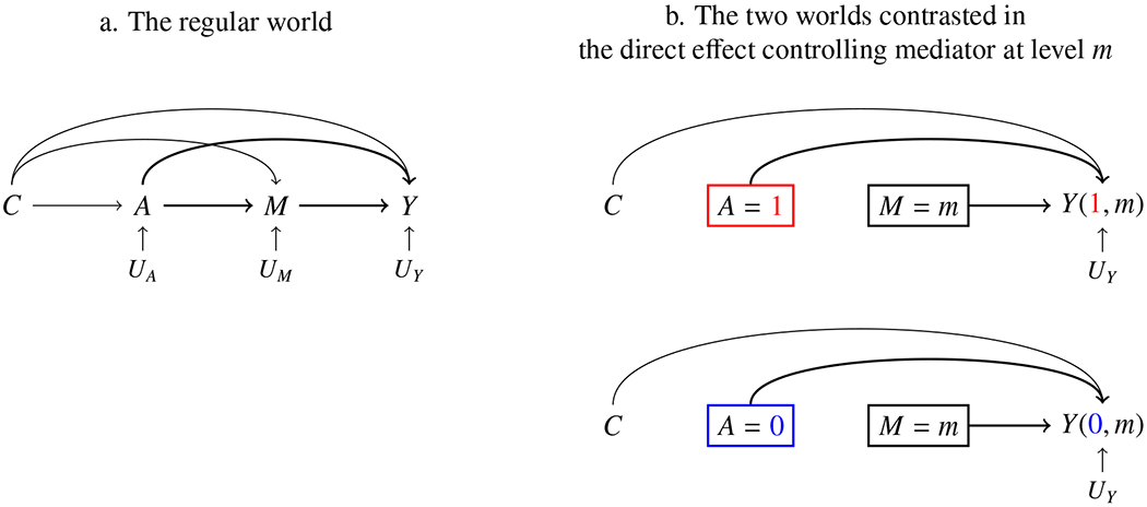
Controlled direct effect

When are CDEs of interest?

CDEs are a type of interventional effect. If a mediator level m is desirable for all and if a feasible and ethical way exists to set it for all, then CDE(m) is relevant. Interventions that shift and fix a variable for a whole population are generally structural, e.g., seatbelt laws, age limits for alcohol/cigarette sale, city-wide water treatment, etc. Consider one last simple example: A city has a successful childhood injury prevention program, and researchers have figured out that a mechanism of the program’s success is that it increased parents’ awareness of burn risks and knowledge of how to set the water heater in their homes to a safe temperature, which shifted the water temperature down on average in households that participated in the program, leading to fewer burns in small children. Recognizing this important effect, the city has passed a bill setting a legal home water heating temperature of maximum 120°F and is planning a blanket intervention sending technicians door-to-door to help set water heaters to under this temperature. The city wants to know whether their childhood injury prevention program would still be effective in the new reality where the burns-due-to-hot-water problem has been taken care of. They are interested in CDE(water temperature = 120).

CDEs (at the population average level) are a special type of GIDEs, where the distribution $\mathcal{D}$ is a single point m. This means that when we are interested in a CDE(m) where m is the desired control mediator level, but suspect that what is obtained would be a range of values that may be centered at m but with some variation, we can simply switch to GIDE(.$\mathcal{D}$) where the distribution [$\mathcal{D}$ is defined to reflect that variation.

This closes the effect definition topic. A summary of the different effect types presented is given in Table 3.

Table 3.

A summary of the effects

Natural (in)direct effects – explaining the total effect
Total effect decompositions	Relevant research questions
direct-indirect: TE = NDE(·0) + NIE(1·)	Does the effect of the college prep program include an indirect (mediated by self awareness) component?
indirect-direct: TE = NIE(0·) + NDE(1·)	Does the effect of the college prep program include a direct (not mediated by self awareness) component?
both	What can we learn about the effect of the college prep program, either through self awareness or through other mechanisms?
Interventional effects – effects of hypothetically modified exposures or hypothetical interventions
Several special effect types	Links to other special effect types
interventional direct effects (IDEs)	paired with IIEs; special case of GIDEs
interventional indirect effects (IIEs)	paired with IDEs
controlled direct effects (CDEs)	special case of GIDEs
generalized interventional direct effects (GIDEs)	contain IDEs and CDEs as special cases
overall interventional effect (OE)	sum of IDE(·0) and IIE(1·); sum of IIE(0·) and IDE(·1)
total effect (TE)	decomposed by natural (in)direct effects
More generally, variation in conditions contrasted
	Examples
set exposure distribution to $\mathcal{D}$A and mediator distribution to $\mathcal{D}$M (most general intervention)	include all the examples below
set exposure to a and mediator distribution to $\mathcal{D}$ (relatively general intervention)	an anti-bullying program that brings the bullying experienced by sexual minority adolescents down to halfway between sexual minority and majority levels the city continuing the injury prevention program plus implementing the city-wide intervention setting home water heating systems to 100-120°F
set exposure to a and mediator distribution to dM(a’)|C (specific intervention)	a hypothetical intervention that brings the bullying experienced by sexual minority adolescents down to the level experienced by sexual majority adolescents modified college prep program without self-awareness components modified college prep program with only self-awareness components
set exposure to a (specific intervention)	college prep program a control condition with some engagement (or a placebo)
set exposure to a and mediator to m (very specific intervention)	the city continuing the injury prevention program plus implementing the structural intervention setting home water heating systems to 120°F the city discontinuing the injury prevention program, but implementing the structural intervention setting home water heating systems to 120°F
no intervention	a no engagement control condition simply observing the bullying experience of sexual minority adolescents

Closing Remarks

The focus of this paper has been the first step in analysis, selecting the target causal effect(s) that reflect the substantive research question. In place of conclusions, we offer a few comments on the next steps – effect identification and estimation – and on settings that are more complex.

Effect identification.

Identification of an effect depends on identification of the mean outcome for each of the two contrasted conditions. Our first comment, as an orientation for readers who are not familiar with this topic, is that there is a hierarchy of difficulty for identification of the mean outcome for different conditions. Identification of the mean outcome for the no manipulation condition is the easiest; it is simply the mean observed outcome. Mean outcome identification for conditions where exposure is set to one value and everything follows naturally (both conditions in TE) is harder, requiring the assumption that exposure assignment is independent of this outcome, possibly given observed preexposure covariates C, usually referred to as no unobserved A-Y confounding. Next up the ladder of difficulty are conditions where exposure is set to one value and mediator is set to one value or a known distribution (both conditions in a CDE), where identification requires an additional assumption: no unobserved M-Y confounding given C, A and intermediate confounders L (if any). If the known distribution is replaced with d_M(a)|C (both conditions in each IDE/IIE), an additional assumption is needed: no unobserved A-M confounding given C. At the top of the difficulty ladder are conditions where exposure is set to one value but mediator is set to its natural value under the other exposure condition (the in-between world in each NDE/NIE), where identification requires that the no unobserved M-Y confounding assumption holds conditional on C only, that is, no intermediate confounders are allowed.³¹ This is a rough summary of a key part of the identification picture. There are details within each of these assumptions that we necessarily gloss over, and there are other assumptions including no interference, consistency, composition, and positivity. We refer the reader to the rich literature, e.g., Avin, Shpitser, and Pearl (2005); Didelez et al. (2006); Imai, Keele, and Tingley (2010); Imai, Keele, and Yamamoto (2010); Pearl (2001, 2012); Petersen, Sinisi, and van der Laan (2006); VanderWeele and Vansteelandt (2009); VanderWeele et al. (2014).

Our second comment concerns the case where the natural (in)direct effects are not identified (due to the presence of intermediate confounders L) but interventional counterparts are. In this challenging case, it may be tempting to simply estimate the latter, even when the scientific interest is in explaining the total effect, that is, in the natural effects. We recommend caution here. VanderWeele and Tchetgen Tchetgen (2017) pointed out that except in rare cases, when an IIE/IDE is non-zero, its natural counterpart is generally also non-zero, which we take to mean that we might consider using the IIE/IDE as proxy for the purpose of testing whether the NIE/NDE is zero. If we are interested in the magnitude of the natural effects that decompose TE, however, the interventional effects are a suboptimal approximation; there is an alternative strategy – see explanations in footnote.³² We also recommend, if one ever uses IDE/IIEs to approximate NDE/NIEs, to be explicit about this approximation, so that there is no ambiguity in the interpretation of analysis results.

Effect estimation.

There is a huge and fast growing literature on estimation, and our comments here are limited. Estimation in the mediation setting can be considered an extension of the non-mediation setting, where estimation of the effect of an exposure on an outcome may rely on an outcome model (e.g., when using regression), or an exposure assignment model (e.g., when using propensity score matching or weighting), or both models (for double robustness). In the mediation setting, if there are no intermediate confounders, estimation of (in)direct effects, and more generally, estimation of effects of interventions that intervene on both the exposure and the mediator, may rely on a combination of two out of three models (a model for the outcome mean, a model for the mediator distribution, and a model for exposure assignment), or all three models for robustness (robustness requires any two of the three models to be correct). With an intermediate confounder, an additional model is required. The methods may involve regression, weighting and imputation; and the term regression is used in a general sense to include both parametric and semiparametric models. We refer the reader to the rich literature, e.g., Daniel et al. (2015); Hong (2010); Hong, Deutsch, and Hill (2015); Imai, Keele, and Tingley (2010); Imai, Keele, and Yamamoto (2010); Lange, Vansteelandt, and Bekaert (2012); Pearl (2012); Rudolph et al. (2017); Tchetgen Tchetgen and Shpitser (2012); Tingley, Yamamoto, Hirose, Keele, and Imai (2014); Valeri and VanderWeele (2013); VanderWeele and Vansteelandt (2010, 2013); Vansteelandt, Bekaert, and Lange (2012); Vansteelandt and VanderWeele (2012).

The models used in traditional mediation analysis are the closest to the estimation strategy that relies on modeling the mediator and the outcome. Two features of traditional mediation analysis deviate from this estimation strategy of causal mediation analysis. First, the outcome model in traditional mediation analysis rarely includes an A-M interaction; causal mediation analysis generally does not impose this restriction. Second, after fitting models, traditional mediation analysis computes the product of coefficients, while causal mediation analysis computes target causal effects. As previously mentioned, these results line up only in special cases.

Since identification requires untestable assumptions – mediators, unlike exposures, cannot be randomized – sensitivity analyses are recommended after, or as part of, effect estimation. See e.g., Ding and Vanderweele (2016); Imai, Keele, and Tingley (2010); Imai, Keele, and Yamamoto (2010) for sensitivity analyses for unobserved mediator-outcome confounding.

More complex settings.

Methods for causal mediation analysis – spanning effect definition, identification, and estimation – of more complex settings is very much an active area of research. We refer the reader to relevant literature. For causal mediation analysis with survival data, see e.g., Didelez (2018); Lange and Hansen (2011); Tchetgen Tchetgen (2011); Valeri and VanderWeele (2015); VanderWeele (2011). For multiple mediators, see e.g., Daniel et al. (2015); VanderWeele and Vansteelandt (2013); Vansteelandt and Daniel (2017). For time-varying mediators and exposures, see e.g., VanderWeele and Tchetgen Tchetgen (2017); Zheng and van der Laan (2017).

To sum up, this paper discusses a key decision in mediation analysis, the selection of the estimand. The proposal is simple and obvious: try to best match the estimand to the research question. The rest of the analysis – including technical aspects of identification and estimation, and the interpretation and discussion of results – resolves around the selected estimand. The causal contrasts presented in the paper, including natural (in)direct effects and a wide range of interventional effects, offer the researcher flexibility, and conceptual clarity, in targeting the knowledge they desire.

References

- Avin C, Shpitser I, & Pearl J (2005). Identifiability of Path-Specific Effects. Proceedings of the International Joint Conference on Artificial Intelligence, Edinburgh, Scotland, 357–363. [Google Scholar]
- Baron RM, & Kenny DA (1986). The moderator-mediator variable distinction in social psychological research: conceptual, strategic, and statistical considerations. Journal of Personality and Social Psychology, 51(6), 1173–1182. doi: 10.1037/0022-3514.51.6.1173 [DOI] [PubMed] [Google Scholar]
- Daniel R, De Stavola BL, Cousens SN, & Vansteelandt S (2015). Causal mediation analysis with multiple mediators. Biometrics, 71, 1–14. doi: 10.1111/biom.12248 [DOI] [PMC free article] [PubMed] [Google Scholar]
- Díaz I, & Hejazi NS (2019). Causal mediation analysis for stochastic interventions. Retrieved from https://arxiv.org/abs/1901.02776
- Didelez V (2018). Defining causal meditation with a longitudinal mediator and a survival outcome. Lifetime Data Analysis. doi: 10.1007/s10985-018-9449-0 [DOI] [PubMed] [Google Scholar]
- Didelez V, Dawid AP, & Geneletti S (2006). Direct and indirect effects of sequential treatments. In Proceedings of the 22nd Conference on Uncertainty in Artificial Intelligence (pp. 138–146). AUAI Press. [Google Scholar]
- Ding P, & Vanderweele TJ (2016). Sharp sensitivity bounds for mediation under unmeasured mediator-outcome confounding. Biometrika, 103(2), 483–490. doi: 10.1093/biomet/asw012 [DOI] [PMC free article] [PubMed] [Google Scholar]
- Frangakis CE, & Rubin DB (2002). Principal Stratification in Causal Inference. Biometrics, 58(1), 21–29. [DOI] [PMC free article] [PubMed] [Google Scholar]
- Geneletti S (2007). Identifying direct and indirect effects in a non-counterfactual framework. Journal of the Royal Statistical Society. Series B: Statistical Methodology, 69(2), 199–215. doi: 10.1111/j.1467-9868.2007.00584.x [DOI] [Google Scholar]
- Glymour C, & Glymour MR (2014). Race and sex are causes. Epidemiology, 25(4), 488–490. doi: 10.1097/EDE.0000000000000122 [DOI] [PubMed] [Google Scholar]
- Hayes AF (2018). Introduction to Mediation, Moderation, and Conditional Process Analysis: A Regression-Based Approach. New York, NY: The Guilford Press. [Google Scholar]
- Holland PW (1986). Statistics and causal inference. Journal of the American Statistical Association, 81(396), 945. doi: 10.2307/2289064 [DOI] [PubMed] [Google Scholar]
- Hong G (2010). Ratio of mediator probability weighting for estimating natural direct and indirect effects. In Proceedings of the American Statistical Association, Biometrics Section (pp. 2401–2415).
- Hong G, Deutsch J, & Hill HD (2015). Ratio-of-mediator-probability weighting for causal mediation analysis in the presence of treatment-by-mediator interaction. Journal of Educational and Behavioral Statistics, 40(3), 307–340. doi: 10.3102/1076998615583902 [DOI] [Google Scholar]
- Imai K, Jo B, & Stuart EA (2011). Commentary: Using potential outcomes to understand causal mediation analysis. Multivariate Behavioral Research, 46(5), 861–873. doi: 10.1080/00273171.2011.606743 [DOI] [PMC free article] [PubMed] [Google Scholar]
- Imai K, Keele L, & Tingley D (2010). A general approach to causal mediation analysis. Psychological Methods, 15(4), 309–34. doi: 10.1037/a0020761 [DOI] [PubMed] [Google Scholar]
- Imai K, Keele L, & Yamamoto T (2010). Identification, inference and sensitivity analysis for causal mediation effects. Statistical Science, 25(1), 51–71. doi: 10.1214/10-STS321 [DOI] [Google Scholar]
- Jackson JW (2019). Meaningful causal decompositions in health equity research: definition, identification, and estimation through a weighting framework. Retrieved from http://arxiv.org/abs/1909.10060 [DOI] [PMC free article] [PubMed]
- Jackson JW, & VanderWeele TJ (2018). Decomposition analysis to identify intervention targets for reducing disparities. Epidemiology, 29(6), 825–835. doi: 10.1097/EDE.0000000000000901 [DOI] [PMC free article] [PubMed] [Google Scholar]
- Jo B, & Stuart EA (2009, oct). On the use of propensity scores in principal causal effect estimation. Statistics in Medicine, 28(23), 2857–2875. doi: 10.1002/sim.3669 [DOI] [PMC free article] [PubMed] [Google Scholar]
- Jo B, & Stuart EA (2012). Comments: Causal Interpretations of Mediation Effects. Journal of Research on Educational Effectiveness, 5(3), 250–253. doi: 10.1080/19345747.2012.688414 [DOI] [Google Scholar]
- Jo B, Stuart EA, Mackinnon DP, & Vinokur AD (2011). The use of propensity scores in mediation analysis. Multivariate Behavioral Research, 46(3), 425–452. doi: 10.1080/00273171.2011.576624 [DOI] [PMC free article] [PubMed] [Google Scholar]
- Judd CM, & Kenny DA (1981). Process analysis: Estimating mediation in treatment evaluations. Evaluation Review, 5(5), 602–619. doi: 10.1017/CBO9781107415324.004 [DOI] [Google Scholar]
- Kennedy EH (2018). Nonparametric Causal Effects Based on Incremental Propensity Score Interventions. Journal of the American Statistical Association. doi: 10.1080/01621459.2017.1422737 [DOI] [Google Scholar]
- Lange T, & Hansen JV (2011). Direct and indirect effects in a survival context. Epidemiology, 22(4), 575–581. doi: 10.1097/EDE.0b013e31821c680c [DOI] [PubMed] [Google Scholar]
- Lange T, Vansteelandt S, & Bekaert M (2012). A simple unified approach for estimating natural direct and indirect effects. American Journal of Epidemiology, 176(3), 190–195. doi: 10.1093/aje/kwr525 [DOI] [PubMed] [Google Scholar]
- Lok JJ (2016). Defining and estimating causal direct and indirect effects when setting the mediator to specific values is not feasible. Statistics in Medicine, 35(22), 4008–4020. doi: 10.1002/sim.6990 [DOI] [PMC free article] [PubMed] [Google Scholar]
- MacKinnon DP (2008). Introduction to Statistical Mediation Analysis. New York, NY: Taylor & Francis. [Google Scholar]
- Mackinnon DP, Fairchild AJ, & Fritz MS (2007). Mediation analysis. Annual Review of Psychology, 58, 593–614. doi: 10.1146/annurev.psych.58.110405.085542 [DOI] [PMC free article] [PubMed] [Google Scholar]
- MacKinnon DP, Kisbu-Sakarya Y, & Gottschall AC (2013). Developments in mediation analysis. In The Oxford Handbook of Quantitative Methods in Psychology: Vol. 2: Statistical Analysis. doi: 10.1093/oxfordhb/9780199934898.013.0016 [DOI]
- MacKinnon DP, & Pirlott AG (2015). Statistical approaches for enhancing causal interpretation of the M to Y relation in mediation analysis. Personality and Social Psychology Review, 19(1), 30–43. doi: 10.1177/1088868314542878 [DOI] [PMC free article] [PubMed] [Google Scholar]
- MacKinnon DP, Valente MJ, & Gonzalez O (2019). The Correspondence Between Causal and Traditional Mediation Analysis: the Link Is the Mediator by Treatment Interaction. Prevention Science. doi: 10.1007/s11121-019-01076-4 [DOI] [PMC free article] [PubMed] [Google Scholar]
- Miočević M, Gonzalez O, Valente MJ, & MacKinnon DP (2018). A tutorial in Bayesian potential outcomes mediation analysis. Structural Equation Modeling, 25(1), 121– 136. doi: 10.1080/10705511.2017.1342541 [DOI] [PMC free article] [PubMed] [Google Scholar]
- Muthén BO (2011). Applications of causally defined direct and indirect effects in mediation analysis using SEM in Mplus. Retrieved from http://www.statmodel2.com/download/causalmediation.pdf
- Muthén BO, & Asparouhov T (2015). Causal effects in mediation modeling: An introduction with applications to latent variables. Structural Equation Modeling, 22(1), 12–23. doi: 10.1080/10705511.2014.935843 [DOI] [Google Scholar]
- NIH. (2016). RFA-MH-17-608: Clinical trials to test the effectiveness of treatment, preventive, and services interventions (R01). https://grants.nih.gov/grants/guide/rfa-files/rfa-mh-17-608.html.
- Pearl J (2001). Direct and indirect effects. Proceedings of the Seventeenth Conference on Uncertainty and Artificial Intelligence, 411–420. [Google Scholar]
- Pearl J (2009). Causal inference in statistics: An overview. Statistics Surveys, 3, 96–146. doi: 10.1214/09-SS057 [DOI] [Google Scholar]
- Pearl J (2012). The causal mediation formula–a guide to the assessment of pathways and mechanisms. Prevention Science, 13(4), 426–36. doi: 10.1007/s11121-011-0270-1 [DOI] [PubMed] [Google Scholar]
- Petersen ML, Sinisi SE, & van der Laan MJ (2006). Estimation of direct causal effects. Epidemiology, 17(3), 276–84. doi: 10.1097/01.ede.0000208475.99429.2d [DOI] [PubMed] [Google Scholar]
- Preacher KJ (2015). Advances in Mediation Analysis: A Survey and Synthesis of New Developments. Annual Review of Psychology, 66(1), 825–852. doi: 10.1146/annurev-psych-010814-015258 [DOI] [PubMed] [Google Scholar]
- Robins JM (2003). Semantics of causal DAG models and the identification of direct and indirect effects. In Green P, Hjort N, & Richardson S (Eds.), Highly Structured Stochastic Systems (pp. 70–81). Oxford, UK: Oxford University Press. [Google Scholar]
- Robins JM, & Greenland S (1992). Identifiability and exchangeability for direct and indirect effects. Epidemiology, 3(2), 143–155. [DOI] [PubMed] [Google Scholar]
- Rubin DB (1974). Estimating causal effects of treatments in randomized and nonrandomized studies. Journal of Educational Psychology, 66(5), 688–701. doi: 10.1037/h0037350 [DOI] [Google Scholar]
- Rudolph KE, Sofrygin O, Zheng W, & van der Laan MJ (2017). Robust and flexible estimation of data-dependent stochastic mediation effects: A proposed method and example in a randomized trial setting. Epidemiologic Methods, 7. doi: 10.1515/em-2017-0007 [DOI] [PMC free article] [PubMed] [Google Scholar]
- Splawa-Neyman J (1923). On the application of probability theory to agricultural experiments. Essay on principles. Section 9 [Translated and edited by D. M. Dabrowska and T. P. Speed]. Annals of Agricultural Sciences, 10, 1–51. doi: 10.1214/ss/1177012031 [DOI] [Google Scholar]
- Tchetgen Tchetgen EJ (2011). On causal mediation analysis with a survival outcome. International Journal of Biostatistics, 7(1). doi: 10.2202/1557-4679.1351 [DOI] [PMC free article] [PubMed] [Google Scholar]
- Tchetgen Tchetgen EJ, & Shpitser I (2012). Semiparametric theory for causal mediation analysis: Efficiency bounds, multiple robustness and sensitivity analysis. The Annals of Statistics, 40(3), 1816–1845. doi: 10.1214/12-AOS990 [DOI] [PMC free article] [PubMed] [Google Scholar]
- Tingley D, Yamamoto T, Hirose K, Keele L, & Imai K (2014). mediation: R package for causal mediation analysis. Journal of Statistical Software, 59(5), 1–38. doi: 10.18637/jss.v059.i0526917999 [DOI] [Google Scholar]
- Valeri L, & VanderWeele TJ (2013). Mediation analysis allowing for exposure–mediator interactions and causal interpretation: Theoretical assumptions and implementation with SAS and SPSS macros. Psychological methods, 18(2), 137–150. doi: 10.1037/a0031034 [DOI] [PMC free article] [PubMed] [Google Scholar]
- Valeri L, & VanderWeele TJ (2015). SAS macro for causal mediation analysis with survival data. Epidemiology, 26(2), e23–e24. doi: 10.1097/ede.0000000000000253 [DOI] [PubMed] [Google Scholar]
- VanderWeele TJ (2011). Causal mediation analysis with survival data. Epidemiology, 22(4), 582–585. doi: 10.1097/EDE.0b013e31821db37e [DOI] [PMC free article] [PubMed] [Google Scholar]
- VanderWeele TJ, & Tchetgen Tchetgen EJ (2017). Mediation analysis with time varying exposures and mediators. Journal of the Royal Statistical Society. Series B: Statistical Methodology, 79(3), 917–938. doi: 10.1111/rssb.12194 [DOI] [PMC free article] [PubMed] [Google Scholar]
- VanderWeele TJ, & Vansteelandt S (2009). Conceptual issues concerning mediation, interventions and composition. Statistics and its Interface, 2, 457–468. [Google Scholar]
- VanderWeele TJ, & Vansteelandt S (2010). Odds ratios for mediation analysis for a dichotomous outcome. American Journal of Epidemiology, 172(12), 1339–1348. doi: 10.1093/aje/kwq332 [DOI] [PMC free article] [PubMed] [Google Scholar]
- VanderWeele TJ, & Vansteelandt S (2013). Mediation analysis with multiple mediators. Epidemiologic Methods, 2(1), 95–115. doi: 10.1515/em-2012-0010 [DOI] [PMC free article] [PubMed] [Google Scholar]
- VanderWeele TJ, Vansteelandt S, & Robins JM (2014). Effect decomposition in the presence of an exposure-induced mediator-outcome confounder. Epidemiology, 25(2), 300–6. doi: 10.1097/EDE.0000000000000034 [DOI] [PMC free article] [PubMed] [Google Scholar]
- Vansteelandt S, Bekaert M, & Lange T (2012). Imputation strategies for the estimation of natural direct and indirect effects. Epidemiologic Methods, 1(1), 7. doi: 10.1515/2161-962X.1014 [DOI] [Google Scholar]
- Vansteelandt S, & Daniel RM (2017). Interventional effects for mediation analysis with multiple mediators. Epidemiology, 28(2), 258–265. doi: 10.1097/EDE.0000000000000596 [DOI] [PMC free article] [PubMed] [Google Scholar]
- Vansteelandt S, & VanderWeele TJ (2012). Natural direct and indirect effects on the exposed: Effect decomposition under weaker assumptions. Biometrics, 68, 1019–1027. doi: 10.1111/j.1541-0420.2012.01777.x [DOI] [PMC free article] [PubMed] [Google Scholar]
- Wright S (1934). The method of path coefficients. The Annals of Mathematical Statistics, 5(3), 161–215. [Google Scholar]
- Zheng W, & van der Laan M (2017). Longitudinal Mediation Analysis with Time-varying Mediators and Exposures, with Application to Survival Outcomes. Journal of Causal Inference, 5(2). doi: 10.1515/jci-2016-0006 [DOI] [PMC free article] [PubMed] [Google Scholar]
Associated Data
This section collects any data citations, data availability statements, or supplementary materials included in this article.