Machine learning and applications in microbiology

ABSTRACT

To understand the intricacies of microorganisms at the molecular level requires making sense of copious volumes of data such that it may now be humanly impossible to detect insightful data patterns without an artificial intelligence application called machine learning. Applying machine learning to address biological problems is expected to grow at an unprecedented rate, yet it is perceived by the uninitiated as a mysterious and daunting entity entrusted to the domain of mathematicians and computer scientists. The aim of this review is to identify key points required to start the journey of becoming an effective machine learning practitioner. These key points are further reinforced with an evaluation of how machine learning has been applied so far in a broad scope of real-life microbiology examples. This includes predicting drug targets or vaccine candidates, diagnosing microorganisms causing infectious diseases, classifying drug resistance against antimicrobial medicines, predicting disease outbreaks and exploring microbial interactions. Our hope is to inspire microbiologists and other related researchers to join the emerging machine learning revolution.

The authors present an introduction to machine learning and its current usage in microbiology with the aim of equipping the reader with ideas and procedural knowledge to apply machine learning to their area of research.

INTRODUCTION

Microbiologists are currently in an era where biological data are collected at unprecedented volumes using high-throughput smart technologies. An escalating skill requirement beyond the laboratory and field experiments is to apply computational techniques to find meaningful information from these data. Machine learning (ML), a core subfield under artificial intelligence (AI), is one proven technique building momentum in the domain of microbiology. It has been used so far in computationally intense problems such as predicting drug targets and vaccine candidates, diagnosing microorganisms causing infectious diseases, classifying drug resistance against antimicrobial medicines, predicting disease outbreaks and exploring microbial interactions. ML has been applied to every microbiology research area including virology, parasitology, mycology and bacteriology.

Over the last five years, there has been a resurgent ML interest from most research areas instigated by the collective capabilities of three advancing technologies: first, devices to rapidly collect large volumes of digital data; second, an exponential increase in affordable computing power and data storage; and third, a global system of interconnected computer networks to rapidly transfer data. The latter technologies are characterised by the terms Big Data, Moore's law and the internet. Popular ML algorithms have been around for decades, but it is these technological ingredients that provided the catalyst for their effective use. This catalyst has opened the floodgate for a surge of ML applications reshaping our lives. Despite now being a well-entrenched term in the scientific community, ML is often perceived as a mysterious and daunting entity to those not in the domain of mathematics or computer science. The aim of this review is to dispel misunderstanding and make ML more accessible to the general scientific community. Our hope is to inspire microbiologists and other related researchers to be productive ML users. This review will be in two parts. Part one is an ML introduction with an emphasis on key points required for an ML user, and part two summarises published examples of how ML has been applied so far to microbiology. The aim of the second part is to provide ideas to new users as to how ML can be applied in their area of research.

What exactly is machine learning?

As humans, we have no problem recognizing a letter ‘A’ mixed among other characters or distinguishing between dog and cat images. This task can easily be performed even if the letter A is written in a style never seen before or the dog and cat images are of unfamiliar breeds. Our ability to perform these tasks has gradually developed over time since our first experience with letters, dogs, and cats. The capacity to learn such tasks improves by an increased exposure to similar experiences. However, despite this capacity, we would struggle to write a procedural set of instructions or rules to perform these and other similar recognition tasks. This is because we distinguish letters, animals or any images by mentally filtering with specific patterns. A skill that we learn unconsciously by experience, but one we are unable to methodically explain.

Before ML, attempts to perform complex tasks like letter and image recognition involved programming computers with rule-based systems. These systems tended to fail outside test scenarios with unseen data. Machine learning has changed the paradigm from programming computers how to perform a task to one where computers learn how to perform the task without being programmed. Importantly, ML algorithms recognize patterns and/or underlying data structure, and not the human programmer. Furthermore, humans typically do not have the mental capacity to define how we consciously visualize these patterns or data structure and consequently, how an ML algorithm exactly performs the task represents a black box to many users. The overarching notion of ML is that humans learn from experience and machines learn from data on how to resolve a complex task. Formal definitions and in-depth explanations of ML are described elsewhere (Mitchell 1997; Flach 2012; James et al. 2013). Machine learning is an extensive field of study that overlaps with and inherits ideas from many related fields such as statistics, computer science and AI. Figure 1 shows the perspective of ML within the AI framework. Machine learning has two main learning modes: supervised (also known as predictive) to make future predictions from training data, and unsupervised (descriptive), which is exploratory in nature without training data, defined target or output (Mitchell 1997). Training data are the initial information used to teach supervised ML algorithms in the process of developing a model, from which the model creates and refines its rules required for prediction. Typically, training data comprises a set of text, images or alphanumerical data that are classified (labelled).

Figure 1.

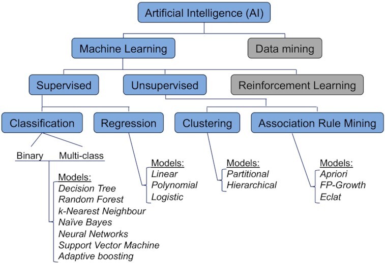
A hierarchical perspective of machine learning within the artificial intelligence framework. Machine Learning (ML)—an application that provides the capacity to automatically learn and improve from experience; Data mining—aims to find useful information from large volumes of data using computer algorithms (not covered in review); Supervised—ML using labelled training data (it can be compared to a human learning in the presence of a supervisor); Unsupervised—ML with unlabelled data (comparable to human learning without a supervisor); Reinforcement learning – focuses on taking a set of actions to maximise reward given a particular environment (requires no training data) (not covered in review); Classification—the task of predicting a discrete class label. A classification model is often referred to as a classifier. Examples of binary classification labels: yes/no, 1/0, vaccine/non-vaccine; and examples of multi-class labels: A, B, C, D for student grades; and teacher, student, secretary, and principal for a school classification; Regression—the task of predicting a continuous quantity; Clustering—an exploratory or descriptive approach in contrast to a predictive approach as in classification and regression; Association rule mining—identifies patterns of association between different variables e.g. movie suggestion, market basket analysis.

Supervised machine learning key terms

Supervised learning can be further grouped into regression and classification. Classification is the process of predicting the category or class of given data points e.g. vaccine candidate or non-vaccine candidate classes. Regression is when the predicted output variable is a real value e.g. predicting antimalarial activity (log IC₅₀). Figure 2A shows observed seroprevalence of a foodborne disease in the human population at different ages. In this case, the disease is caused by food contaminated with bacteria and seroprevalence is the proportion of individuals who have been exposed to the bacteria evidenced by the presence of anti-bacterial antibodies in their serum. There are only eight fictitious measurements for the purpose of illustration, but in reality, ML is a tool for analysing complex and/or voluminous data. Our task is to predict the seroprevalence given any age. A simple solution would be to draw a line that best fits the data as in Fig. 2B. The positioning of the line represents an attempt to achieve the minimum distance from the line to each data point. The ML approach is to find a model that best fits the data. In effect we fit a model to past data to be able to predict future data. A caveat here is that future data must be similar to past data in order to correctly make predictions. In this illustration, the classic formula for a straight line is an appropriate model because it clearly defines a relationship between seroprevalence and age. Fig. 2C shows the formula and how its components are termed by ML convention. In ML terms, ‘prevalence’ is the label and ‘age’ is the feature (or predictor). A label is what we are trying to predict and a feature is what we use to help make the prediction. Only one feature is represented here, but millions of features could be used in more complex ML projects. The straight line formula represents a type of regression model, which can be used to predict a continuous value from a linear combination of input features. An example in the ML context is a particular instance of known or past data. Eight labelled examples consisting of both the feature and the label are given in this instance. We use labelled examples to train the model. That is, the labelled examples empower the model to learn the relationship between the feature(s) and label. These labelled examples represent the training data. The supervised learning here involves determining the optimum values/parameters for the weight (slope) and bias (Y-intercept) given the training data.

Figure 2.

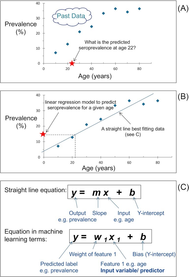
(A) Scatter plot showing observed seroprevalence of a foodborne disease in the human population at different ages. It highlights, as an example, the task of predicting the prevalence at age 22. (B) Same data as scatter plot ‘A’ but displays a line that best fits the data. This line represents a simple manual solution to solving the task. (C) The machine learning solution is to find a model that best fits the data. For this example, a straight line formula is an appropriate model, which predicts ‘y’ for a new value of ‘x’. Components of the straight line formula (a linear regression model) are also shown in machine learning terms, whereby the linear regression ‘machine learning’ model predicts a value for an input given past data. This model only has one feature e.g. age. Millions of features could theoretically be used.

In effect, learning in a supervised ML sense is attempting to minimise loss. Loss is a value determined by a loss function and can be an empirical or structural component. An empirical component indicates how well a model performed on a single example (0 = perfect prediction). For example, if the line in Fig. 2B was a perfect predictive model, all example data points would be on the line and the loss would be zero. In other words, the point's position relative to the line is an indication of loss. A structural component indicates the complexities of the model e.g. complex models have many parameters giving a high structural loss and simple models have few parameters giving a low structural loss value. Machine learning approaches typically exploit common mathematical functions that aggregate individual losses into one informative value. These types of functions are termed loss or cost functions. The aim of an iterative ML learning process is to determine (learn) the optimum parameters that have minimum loss, on average, across all data points e.g. a set of weights and biases that have minimum loss in Fig. 2B.

An ML algorithm, unlike a human, has no prior intuition to fit a straight line as close as possible to all plotted data points such as those shown in Fig. 2A. As far as the algorithm is concerned, there are a multitude of possible biases and weights. One iterative approach to learning the optimum parameters through a ML training process involves initially using random values for the bias and weight. The loss is then calculated. In this instance, the perpendicular distance from each example data point to the random line is measured. Distances are squared and summed to calculate an indication of loss i.e. the method of least squares is applied, which is one example of a loss function. The process of iterating over the training data with newly generated or modified parameters is repeated until the algorithm discovers the model parameters with the lowest loss (see Fig. 3). Calculating the loss function for every conceivable weight and bias is feasible but inefficient. A more efficient method is called gradient descent (Gardner 1984; Mitchell 1997) (see Box 1), however this method may not converge to the best solution. A trained model is one with parameters having the lowest loss, on average, when applied to all labelled examples. An important next step is to apply evaluation measures on test data as an indication of how well the model might predict with future data. This is typically achieved by using labelled examples (e.g. data with known seroprevalence and ages) not previously used in training. That is, the trained model predicts or infers values (e.g. seroprevalence) given input data (e.g. ages) with already known target values (e.g. seroprevalence). Then, evaluative comparisons/measures can be made between predicted and true values to assess the predictive capacity of the model (see later section on ‘Evaluation measures’). An Achilles' heel of supervised ML is overfitting (see Box 2).

Figure 3.

A typical interactive cycle for training a supervised machine learning model. The diagram represents one cycle of training (i.e. create model, predict, test and generate model parameters). For illustrative purposes, the training cycle is applied to a linear regression model. Cycles are repeated until the parameters have the lowest loss when applied to all training data.

Box 1: –Gradient descent.

Gradient descent approaches are iterative algorithms (based on a convex function) used when training a machine learning model to find model parameters with the lowest loss using only local information. Starting with a random initial set of parameters, they change the parameters slightly in the direction that leads towards lower loss. After repeating this over many iterations, gradient descent will identify either the global minimum value (i.e. the lowest point in the entire function) or a local minimum (i.e. a point which is lower than the surrounding area of the function). The aim is to find the global minimum and therefore gradient descent approaches use various schemes to escape from local minima, such as adding a small amount of noise to the parameter change or adding a momentum term where the parameter change is the sum of the direction minimising loss and the direction in previous iterations.

Box 2: –Overfitting and Bias-Variance Tradeoff.

Overfitting occurs when a model fits the training data too well (e.g. gets a low loss during training) and does not generalize to examples not seen by the model during learning (e.g. poorly predicts given new data). There are primarily two error components called bias and variance. Bias can be thought of as prediction error due to assumptions in the model. In Fig. 2, a linear relationship between the target (e.g. seroprevalence) and the feature (e.g. age) was assumed. The straight line formula might not be capturing the true relationship. The inability of a ML model to capture true relationships between a target and features represents the bias component. A high bias ML model signifies underfitting i.e. a high inability to capture true relationships. In contrast, an ML model consisting of a squiggly line traversing all points in the training data would have low bias.

The variance is a measure of the sensitivity of an ML model to different datasets e.g. high variance would be observed if there was a significant difference between performances using training and test data. A high variance ML model signifies overfitting e.g. the former squiggly line model that is very sensitive to a particular dataset. As model complexity (i.e. parameter numbers) increases, bias tends to decrease and variance increase. Conversely, bias increases as variance decreases. The aim is to find that sweet spot between a simple model and a complex model that warrants a bias-variance tradeoff to avoid overfitting and underfitting conditions. Popular ways to obtain the optimal bias and variance for an ML model are generalizing training data, regularization (a technique penalising complex models), and using ensemble methods. A workable ML model may transpire only making satisfactory rather than great predictions when training but, in compensation, should deliver consistently satisfactory predictions on new data.

Unsupervised machine learning key terms

Unsupervised learning requires no prior knowledge or training data. The ML input data contains only features with no labels i.e. unlabelled examples. In a microbiological context, the bulk of unsupervised ML applications involve clustering or dimensionality reduction/ordination algorithms. Clustering is a commonly used technique of unsupervised learning to identify patterns in highly dimensional data by finding data clusters such that each cluster has the most closely matched data. Dimensionality refers to the number of features in a dataset and high dimensional data denotes a large number e.g. the number of features exceeding the number of observations.

Clustering procedures can be divided into two major types: hierarchical and partitional.Hierarchical clustering is when the identified clusters are subsets of larger clusters i.e. nested clusters, typically represented as a cluster dendrogram. Partitional clustering is when the identified clusters do not overlap (i.e. un-nested clusters).

In most cases, algorithms for unsupervised ML are provided with a highly dimensional dataset in the form of a dissimilarity matrix. A dissimilarity matrix is a pairwise table commonly used as the input for various clustering and dimensionality reduction procedures e.g. the table contains column headings and row headings indicating the name of each specimen in a biological dataset, and the cell produced at the intersection of a row and column for any pair of specimens contains a dissimilarity metric (often a number between 0 and 1, reflecting the level of dissimilarity between the two specimens). The type of dissimilarity measure depends greatly on the context e.g. in microbiological contexts, the measure may be calculated by simply normalising the number of reads mapping to genes that are shared between taxa (or populations) of interest, or calculation of more sophisticated indices such as genetic distances based on Nei's algorithm (Nei 1972), fixation index (F_ST) (Holsinger and Weir 2009), the Jaccard Index (Jaccard 1912), or Bray-Curtis dissimilarity (Bray and Curtis 1957).

Typically, when a highly dimensional dataset is provided in the form of a dissimilarity matrix, a dimensionality reduction (ordination) procedure is required. This unsupervised ML procedure reduces the highly dimensional dataset to a set of coordinates in two- or three- dimensional space, allowing visualisation of relationships among specimens included in the dataset. For example, partitional clustering is often applied to 2D/3D sets of coordinates such as those generated by a dimensionality reduction procedure to identify the points that most appropriately group into a number of ‘k’ possible labels. There are numerous dimensionality reduction methods (Huang, Wu and Ye 2019; Velliangiri, Alagumuthukrishnan and Joseph 2019; Xu et al. 2019) and clustering procedures (Saxena et al. 2017; Perez-Suarez, Martinez-Trinidad and Carrasco-Ochoa 2019) and while the algorithms underpinning them may be quite different, the general objective is the same; to identify subgroups of a dataset that share sets of important biological features.

One popular partitional clustering method for distinguishing groups is k-means clustering (an unsupervised algorithm). Figure 4 shows its algorithmic steps. The ‘k’ in k-means clustering is the number of desired groups/clusters. A trial and error method could be used to determine ‘k’ but it is straightforward to use metrics which favour well-separated, dense clusters such as the Silhouette Coefficient (Rousseeuw 1987) or the Davies–Bouldin Index (Halkidi, Batistakis and Vazirgiannis 2001). The user should choose the ‘k’ giving the maximum value of the metric. Table 1 highlights the main differences between supervised and unsupervised ML.

Figure 4.

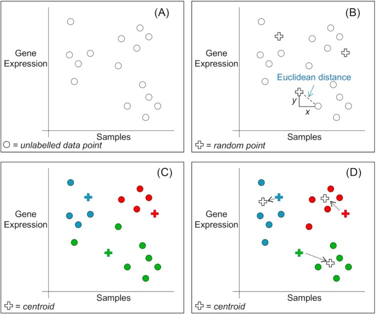
(A) Shows gene expressions taken from fictitious microbial samples. There are 15 unlabelled data points for the purpose of illustration. Our task is to group the samples for further analysis. We can easily distinguish three groups, but an ML algorithm has no intuition. One popular partitional clustering method for distinguishing groups is k-means clustering (an unsupervised algorithm). The first step is to select the number of desired groups/clusters (i.e. the ‘k’ in k-means clustering). (B) Shows the same data as ‘A’ but with three randomly selected points as initial centroids for the three desired clusters e.g. k = 3. A distance is measured between the centroids and every data point (a common distance measurement is the Euclidean i.e. √x² + y² for two dimensions). (C) Each data point is assigned to the cluster associated with nearest centroid (i.e. choose minimum distance). (D) Three new centroids are computed using the mean of the data points within the cluster and then once more, each data point is assigned to the cluster associated with nearest centroid. This process is repeated until the centroids do not move (i.e. stop when clustering process has converged).

Table 1.

Comparison between supervised and unsupervised machine learning.

	Supervised ML	Unsupervised ML
Initial data	Prior knowledge (labelled examples) of the expected type of output e.g. input variables (features) and known output variable (label).	No examples of the expected type of output e.g. only input variables (features)
Goal	Predict the classification or values of unseen data e.g. given new input data (features) predict output variables (label).	Model the underlying structure or distribution in the input data to detect novel patterns that are difficult or impossible to detect by manual human observation.
Method	Statistical patterns are searched for within labelled examples (i.e. training data) using algorithms designed to detect similar patterns in unseen/future data. This algorithm learning method using training data can be thought of as a teacher supervising the learning process.	Unsupervised algorithms group unsorted/unordered information based on similarities and differences. These algorithms have no prior knowledge or training. The unsupervised learning process can be thought of as learning without a teacher.
Example	A dog image is not a random collection of pixels. There is a pattern specific to a dog. The more examples, the more finely tuned the algorithm becomes in learning the relationship between the features (pixels) and label (dog image), and the more accurate it can be in performing the classification task.	Given unsorted pixels of cats and dogs, unsupervised algorithms attempt to figure out on their own how to sort them according to similarities, relationships, and differences even when the algorithm has no notion of the type of categories to expect.
Expected output	Correct answers are known in the form of training data. The ML algorithm iteratively makes predictions on the training data to determine (learn) optimum algorithm values/parameters. Learning stops when the optimum attains an acceptable minimum difference (loss) between prediction and correct answer.	No training data so correct answers are typically unknown. ‘Appropriate interpretation of results’ and ‘validation that the algorithm has solved the intended problem’ is at the discretion of the user.

ML = machine learning

Typical steps in a supervised machine learning project

Supervised ML projects typically have similar steps to the following:

1. Gather labelled examples—the quality and quantity of data directly determines the accuracy of the predictive model. Predictions will be inherently flawed if the input data is flawed, irrespective of the algorithm used. A guiding rule is that the more generalised examples you have representing the problem domain, the better the outcome. Generalization refers to how well the trained ML model will perform on previously unseen data drawn from the same distribution as the one used to create the model.

2. Extract features from example data and collate in a table in a similar manner to Fig. 5. Example data is not always available in its purest form and invariably contain unwanted spurious data (noise) that do not represent true data properties from the problem. Some ML algorithms handle noise better than others.

3. Prepare data—initial raw data are seldom perfect and generally require preparation before ML algorithms will run appropriately and/or yield useful predictions (see Box 3).

4. Split data—typically the data is randomly divided into two sets. One set contains the majority of data e.g. 80% and is used for training the ML model. The other set e.g. 20% is used to evaluate the model's performance. The same data should never be used for training and evaluation. Alternatively, the data might be split into three sets: train/test/cross-validation. Cross-validation is for parameter setting (see Box 4).

5. Choose a model—there are several choices of ML models that can solve the same problem. Each model is supported by diverse algorithm approaches and will perform differently on different datasets. It is a learnt skill to choose the appropriate model for the problem. No one model is better than others on all classes of problems. The recommendation is to apply several models and determine which model performs best on evaluation data. However, the following factors tend to dictate the model choice: type of problem; size, quality, and datatype of training data; computational hardware available; required accuracy, ease of implementation; desired and urgency of output; and necessary level of interpretability of how output was achieved.

6. Train the chosen model—this is the crux of ML as it is the iterative process of incrementally improving the model's ability to predict (See Fig. 3).

7. Evaluate trained model—use the evaluation data to evaluate how the model performs on data not yet seen as a proxy of how the model might perform in the real world.

8. Refine the model parameters—this optional step is dependent on how well the model performed in evaluation. Further training may be required with updated examples, an increased number of training steps, and/or different starting parameters. Finding the optimum model parameters can be more of an art and an experimental process, especially for complex models.

9. Make predictions using the trained model on real world data and ideally, the predictions can be verified by independent methods. For example, a ML predicted vaccine candidate could be tested in a laboratory. In reality, conclusively verifying predictions may be logistically or financially restrained. The best compromise is ensuring that the trained model itself is thoroughly evaluated and performs well.

Figure 5.

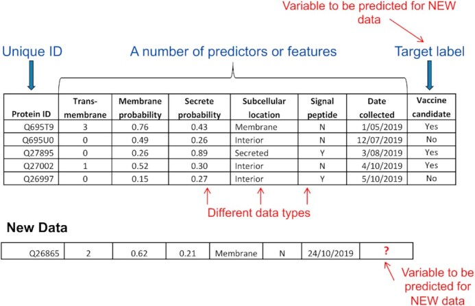
Example of training/example data in a table format for supervised learning. Here, data has been gathered to classify the vaccine candidacy potential of proteins against a target pathogen. This is an illustration of classification data for supervised learning. Each column contains a specific output value from bioinformatic programs that predict protein characteristics given protein sequences. There are six features or predictors (except ‘Date collected’ is a spurious feature). Machine learning (ML) algorithms can exploit a generalised pattern within the collection of labelled features (i.e. features with known target labels) to classify an unlabelled protein (i.e. new data) that has the same features. In reality, the features that contribute or debilitate the prediction are not usually known. Therefore, training data invariably contain debilitating features (e.g. Date collected) that are termed ‘noise’ in ML. Some ML algorithms (e.g. decision trees) are flexible in terms of input data types (e.g. categorical, binary and numeric), whilst some (e.g. artificial neural networks) expect only numerical input and others (e.g. some versions of Naive Bayes classifier) expect categorical. Hence, appropriate data type transformations may be required.

Box 3: –Data preparation.

Machine learning input data is typically represented in a table format—records (rows) and fields (columns). Initial raw data is seldom perfect and can have missing or incomplete data values, outliers or anomalies, and incorrectly formatted data. The process of detecting and correcting (or removing) corrupt, inaccurate, incomplete or irrelevant raw input data is referred to as data cleansing. In most cases, the data may need deduplication, normalisation, transformation and removal of errors. Normalisation is a technique often applied when features in the dataset have different ranges e.g. numeric columns can be changed to a common scale without distorting differences in the value ranges (ultimately, the goal of normalization is to separate biologically meaningful signal from other confounding signal sources).

Whilst some ML models, such as random forest or decision trees take missing data into their stride, others such as neural networks or support vector machines cannot. For these cases and depending on the amount of missing values, the missing data may be handled by imputing it from the remainder of the dataset, or setting the missing values of a feature to the mean or mode value. Some algorithms may also require converting categorical data to numerical equivalents e.g. representing week days as 1, 2 instead of Monday, Tuesday etc. Furthermore, it is recommended to randomize the order in the table. One column in the table is designated the target label and requires a mandatory value. Ultimately, the target is the variable to be predicted in new data. Ideally, there should be an equal number of rows representing each possible target classification. Algorithms still function with unequal numbers of target classifications but the caveat is that typically the more unequal, the more bias towards making classifications in favour of the majority class.

Box 4: –Cross-Validation.

k-fold cross-validation is a resampling statistical method used to estimate the performance of machine learning models. The ‘k’ refers to the number of groups that a given data sample is to be split e.g. 5-fold cross-validation indicates the sample data is split into five. The typical steps required are (i) split a randomly shuffled dataset into k groups; (ii) hold one group as a test dataset and use the remaining groups as a training dataset; (iii) fit a model on the training set and evaluate it on the test set and (iv) repeat steps two and three until each group has been used as the test set. The average of the k evaluation scores provides an indication of how the model is expected to perform when used to make predictions on data not used during model training. This validation method gives an underestimate of performance because by convention the operational/application model will contain 100% of the example data and is expected to perform slightly better than the cross-validation estimate suggests.

Leave-One-Out (LOO) cross validation is a statistical method similar to k-fold cross validation but is more suited to small datasets. The ‘k’ in LOO terms is equal to the number of data points in the sample data set. In effect, the model is trained on all the example data except for one point and then the trained model validation is performed only on this left out point. This latter procedure is repeated k-fold and an average is computed for the performances.

It is instructive to compare validation using a holdout set with the above cross-validation methods. Validation with a holdout set involves randomly splitting the data into a training portion and a test portion (often a simple 80/20 split). The model is built using the training split and evaluated on the test split. This approach is faster than k-fold or LOO cross-validation because only one model is trained, but the performance estimate is less robust because it is evaluated on only one sample of the data that may be either particularly easy or difficult to classify than the average. With large datasets, where the holdout set is representative this approach may be valid. In situations where models require large amounts of computing power to train, it may be impractical to build the many models required for k-fold or LOO cross-validation.

Typical steps in an unsupervised machine learning project

Unsupervised ML aims to detect novel patterns in data that are difficult or impossible to detect by manual human observation. This category of ML is considered ‘unsupervised’ because the algorithms used do not require a set of labelled examples for training prior to analysis. Clustering (synonym: unsupervised classification) is arguably the most widely applied category in unsupervised ML. Therefore, the following steps describe typical preparations taken as part of a clustering project:

1. Gather labelled examples if possible—in the context of unsupervised ML, labelled examples are not used to train a model but are used instead to evaluate clustering performance downstream.

2. Extract features from example data—collate these features in a table in the same manner described for supervised ML.

3. Prepare data—depending on the context this will involve similar data curation steps described for supervised ML. However, for unsupervised ML this step will also require selection of suitable distance (or dissimilarity) metrics calculated from the extracted data features. The metric used will depend on the application. Once an appropriate metric is selected, distances are calculated between every possible pair of specimens in a dataset. The result is usually represented as a pairwise matrix of values that is usually the input for the chosen clustering model.

4. Choose a model—there are several clustering models that can be applied to a given distance matrix and the model selected will depend on the purpose (Rokach 2009). Identification of an appropriate model is usually achieved through comparison of several models.

5. Select a value for k—the constant k represents the number of expected clusters (which may also be thought of as the number of labels). There are several ways to select an appropriate value of k (Xu and Tian 2015), and this can drastically impact the interpretation of which specimens/objects in your dataset possess the same label. For example, when using a hierarchical clustering model, each cluster is actually a subset of a larger cluster, which does not serve well for assigning a discrete label to each specimen. Selecting a value for k forces the model to assign specimens to any one of k possible labels.

6. Evaluate clusters—use labelled examples from step 1 (if available) to determine whether the model has assigned specimens of the same label to the same cluster. This can facilitate calculation of various evaluation measures (see below).

Evaluation of models

A critical step in developing a supervised and unsupervised ML model is to evaluate the performance at training (supervised) and testing stages (supervised and unsupervised) to validate that the model is solving the correct problem and to verify the model is robust. In other words, that the predictive model is likely to generalise to unseen data or that the clustering is complete and consistent. Validation that the model is solving the correct problem is in the hands of the user. Verification that the model is robust and produces the correct results can be done theoretically or empirically. Theoretical verification, for example, by proving that a neural network produces the correct results is out of the scope of this paper. Mostly, an empirical validation is done by applying appropriate statistical measures to record the performance and evaluate the capacity of the model to generalise correctly. Evaluation measures are essential for comparing different models given varying permutations of algorithm types, parameters, and feature combinations. The purpose of this evaluation is to find the optimum permutation for the application. Some common evaluation measures and terms, also reviewed in (Handelman et al. 2019), are True Positive (TP), False Positive (FP), True Negative (TN), False Negative (FN), Accuracy (ACC), Misclassification or Error Rate; True Positive Rate (TPR) or Sensitivity (SN) or recall, False Positive Rate (FPR), True Negative Rate (TNR) or Specificity (SP), Precision or Positive Predictive Value (PPV), Negative Predictive Value (NPV), and Prevalence (see also Fig. 6). F1 Score (or F-measure), and Area Under the Curve (AUC) are also popular measures. F1 Score is the geometric mean of precision and recall. AUC is the percentage under a Receiver Operating Characteristic (ROC) curve, which represents a single value ranging from 0 to 1 summarising the classifier performance e.g. 1 is perfect, 0.5 poor. ROC Curve is a graph showing TPR (y-axis) against FPR (x-axis), which summarizes the performance of a binary classifier for every possible classification threshold.

Figure 6.

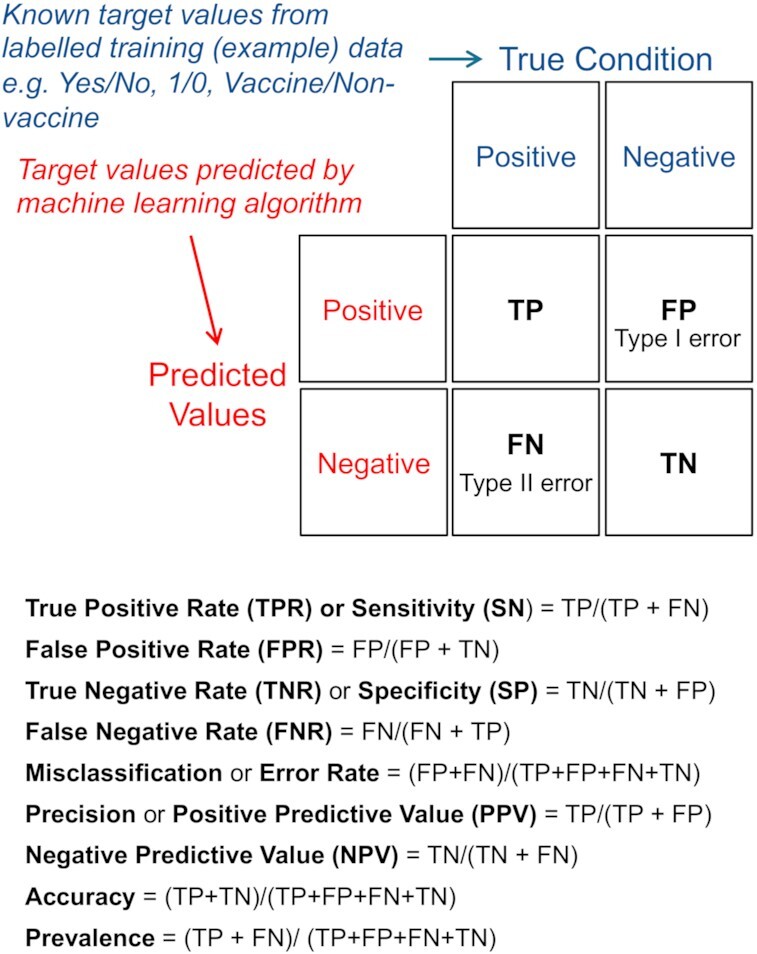
Confusion Matrix. The example shown is for a binary classifier. A confusion matrix can, however, be extended to have more than two classes. TP = true positive (true condition correctly identified as true e.g. predicted Yes and true condition is positive). TN = true negative (negative condition correctly identified as negative e.g. predicted No and true condition is negative). FP = false positive (predicted value is positive but true condition is negative—also known as ‘Type I error’). FN = false negative (predicted value is negative but true condition is positive—also known a ‘Type II error’). True Positive Rate (TPR) or Sensitivity (SN) = how often the classifier correctly predicts a positive condition when the condition is positive. False Positive Rate (FPR) = when the condition is negative, how often the classifier incorrectly predicts a positive condition. True Negative Rate (TNR) or Specificity (SP) = how often the classifier correctly predicts a negative condition when the condition is negative. False Negative Rate (FNR) = when the condition is positive, how often the classifier incorrectly predicts a negative condition. Misclassification or Error Rate = how often the classifier is incorrect. Precision or Positive Predictive Value (PPV) = how often is the prediction correct when the classifier predicts a positive condition. Negative Predictive Value (NPV) = how often is the prediction correct when the classifier predicts a negative condition. Accuracy (ACC) = how often the classifier is correct. Prevalence = how often the positive condition occurs in the sample.

Empirical evaluation of a supervised ML model involves comparing the predictions of the model with the known actual results and deriving metrics, like those above, which express the quality of the model. It is important that the comparison is made on a dataset not used to train the ML model. Otherwise, the quality of the model will appear to be higher than it would be when used on new data. Consequently, a holdout (or test) set is commonly used, or some form of cross validation is applied such as k-fold cross validation or Leave-One Out cross validation (see Box 4). For classification problems, a confusion matrix containing TP, FP, TN and FN values is commonly computed (see Fig. 6). From this, for binary classification problems, other measures such as accuracy, error, and the other measures listed above may be computed. In unbalanced classification problems, where the number of examples of classes are unequal, accuracy and misclassification rate are unsuitable. Instead, SN, SP, precision, recall, the F1 score or AUC are more appropriate because they are unaffected by the differences in number of cases of each class. Furthermore, Precision-Recall (PRC) plots can provide visual performance representations for unbalanced classification problems (He and Garcia 2009; Saito and Rehmsmeier 2015). Multi-class classification problems can be dealt with by treating them as sets of binary classification problems. For example, one class vs the other classes. Then the measures can be averaged over the binary problems potentially weighted by numbers of data points in each class. For regression problems, measures such as mean squared error or root mean square error are appropriate; essentially measuring the distance the predicted value is from the actual, averaged over the test examples.

Evaluating unsupervised ML models is not a trivial matter. The absence of labelled examples in many circumstances means there is nothing to which the model's results can be meaningfully compared i.e. there is typically no ground truth. While it still remains subjective, one compromise is to test how well the unsupervised algorithm performed in the context of the desired end goal. As an example, the Silhouette measure (Rousseeuw 1987) can be used to evaluate clustering results on data when the ground truth is unknown. It does this by measuring the intra-cluster distance (i.e. how close each data point within each cluster is to every other data point in the same cluster) and the inter-cluster distance (i.e. how close each cluster of data points is to other clusters). Relatively small intra-cluster distances and relatively large inter-cluster distances are an indication the algorithm performed well in grouping the data points, but not an indication that the grouping correctly represents underlying data structure. Box 5 provides an evaluation example when ‘ground truth’ exists.

Box 5: –Evaluating an unsupervised machine learning procedure against ‘ground truth’.

For the purposes of assessing clustering performance, ground truth labels may be assigned to specimens using easy-to-observe features that satisfy two prerequisites: (i) are unrelated to the features forming the basis of clustering, and (ii) should nonetheless result in assignment of specimens to the same label. As an example, evaluating different sequence clustering procedures using data generated for a collection of protein coding genes from various vertebrates (e.g. mammals, birds, reptiles, amphibians and fish), can be achieved using these five invertebrate groups as labels. We can easily assign one of these labels to any given vertebrate on the basis of clear physical differences. The more robust clustering procedure will assign a set of homologous gene sequences from ducks, chickens, frogs, salamanders, wolves, sheep, snakes, lizards, sharks and goldfish, to their appropriate ground truth label at a higher rate than a poorly performing clustering procedure. In the context of molecular surveillance methods for microbial pathogens, a similar strategy could be to use epidemiologically defined clusters of illness as ground truth labels to assess how well a genetic clustering procedure performs (Barratt et al. 2019a), given that infections derived from a common source of exposure are typically caused by the same strain of microbe. A robust clustering procedure will group specimens with the same epidemiologic label together at a high rate based solely on the genetic features identified for the same specimens.

Popular machine learning algorithms

There are many machine learning algorithms. These are the sets of rules that steer the ML process to identify patterns in data, build models, and make predictions without having explicit pre-programmed rules. The goal of supervised ML algorithms is to separate the classes. To help conceptually appreciate class segregation, a step by step hand approach in constructing one decision tree model is illustrated in Supplementary information 1. Eight popular supervised ML algorithms are logistic regression (LR), decision tree (DT), random forest (RF), k-nearest neighbour classifier (kNN), naive Bayes classifier (NB), artificial neural networks (ANN), support vector machine (SVM), and adaptive boosting (adaBoost). Summaries of these algorithms are described in Supplementary information 1. Deciding which algorithm to apply to a particular problem is the main challenge to a new ML user. This challenge, nevertheless, can be overcome by testing all popular algorithms and selecting the one with the best performance evaluation. Alternatively, all or several algorithms can be used as an ensemble of classifiers (See also Box 6 ‘Accuracy and Explainability’, Box 7 ‘Prediction versus Inference’).

Box 6: –Accuracy and Explainability.

The most accurate ML predictions are typically made by black-box models i.e. no clear explanation provided as to how or why the model made a certain prediction. Conversely, predictions from so-called white-box models are comparatively easier to interpret but are notably less accurate (London 2019). The outcome of this predictive accuracy or explainability tradeoff is essentially at the ML user's discretion in their ML model choice deemed to be the most applicable to the given problem. For example, model interpretability may be crucial in explaining why the independent input features predict the dependent attribute; or equally, the priority may call for absolute precision even if the model spits out a result with no explanation. One approach sometimes used is to build a black-box model, using for example an artificial neural network, to provide an accurate result then to train a white-box method such as a decision tree to explain the results of the back-box method (Guidotti et al. 2019). Explainability in AI is a current research focus including recent methods such as Local Interpretable Model-agnostic Explanations (LIME) (Ribeiro et al. 2016), which builds local models to explain specific black-box predictions, or Saliency Maps (Fong, Vedaldi and Ieee 2017), which highlight the parts of an image that explain the ML model's classification.

Box 7: –Prediction versus Inference.

Related to accuracy and explainability of models is prediction and inference. These relate to how the resulting model is intended to be used. Prediction is when the user wants to predict the class or value for a new data point but does not care about how the input parameters affect the output. Highly accurate models are useful in this situation. In contrast, inference is when the user wants to understand more about the data generation process. They want to understand how the model output is affected by changes in the model inputs. In this case, the explainability of the model is paramount and models such as logistic regression or Bayesian approaches are applicable. It is possible to have a highly predictive (i.e. accurate) model, but this may not be suitable or meaningful for inference.

Popular unsupervised learning algorithms are k-means for clustering and Apriori algorithm for association rule mining (Hipp, Güntzer and Nakhaeizadeh 2000). The goal of unsupervised ML algorithms is to find hidden relationships between data objects and structure objects by similarities or differences. Consequently, dimensionality reduction procedures such as t-distributed stochastic neighbour embedding (t-SNE) (Cieslak et al. 2020), Uniform Manifold Approximation and Projection (UMAP) (McInnes and Healy 2018)—an approach possessing some advantages over t-SNE (Becht et al. 2019), and other ordination methods such as GOMMS (van der Maaten and Hinton 2008; Sohn and Li 2018) also constitute forms of unsupervised ML.

Publically available software for machine learning applications

All popular ML algorithms are freely available online. Table 2 lists available open source software designed totally or partially for machine learning. Most are open source and are provided within software libraries e.g. Scikit-learn, TensorFlow, PyTorch, Theano, Microsoft Cognitive Toolkit, and Keras in Table 2 are Python frameworks (a collection of libraries) that allow a user to build ML models without in-depth knowledge of the underlying algorithms. However, knowledge of how the algorithms work will help with interpretation of output and choice of evaluation method. Software libraries may present a challenge to users with limited programming ability because their interface requires modifying programmable scripts e.g. Python or R languages. However, programming a script from scratch is a rarity as library developers provide a ready-made framework of easily modifiable scripts to access the libraries. Machine learning algorithms are also accessible for users with no programming experience through tools such as the KNIME Analytics Platform, which promotes ‘visual’ programming, or Weka.

Table 2.

Publically available software for machine learning applications [websites last viewed in October 2020].

Application Name	Primary machine learning models	URL
Scikit-learna	Classification, regression, clustering	https://scikit-learn.org/stable/index.html
WEKA	Classification, regression, clustering	https://www.cs.waikato.ac.nz/ml/weka/
KNIME	Classification, regression, clustering	https://www.knime.com/
TensorFlowa	Neural networks	https://www.tensorflow.org/
Kerasa	Neural networks	https://keras.io/
Microsoft Cognitive Toolkita	Deep learningb	https://www.microsoft.com/en-us/cognitive-toolkit/
PyTorcha	Deep learningb	https://pytorch.org/
Theanoa	Deep learningb	http://www.deeplearning.net/software/theano/
Caffe	Deep learningb	http://caffe.berkeleyvision.org/

^aPython frameworks (a collection of libraries, which are specific files containing pre-written code that can be imported into user's Python code).

^bDeep Learning is essentially working with large neural networks (‘deep’ typically refers to the number of layers).

WEKA—a collection of ML algorithms that can either be applied directly to a dataset or called from Java code written by a user.

KNIME—a GUI-based workflow platform that allows a user to drag-and-drop various pre-built machine learning modules without writing programming code. However, user code written in R and/or Python can be integrated in a KNIME analytical workflow.

Caffe—an open-source Deep Learning framework that supports interfaces such as C, C++, Python, MATLAB, and Command Line interfaces (CLI). However, familiarity with C++ is required.

Machine learning algorithms are additionally provided through R packages. Although running the packages demand knowledge of R command-line syntax, no programming expertise is required. Table 3 lists relevant R packages. Rattle is a graphical user interface (GUI) for data mining using R (Williams 2009). A key feature is that all performed GUI interactions are recorded as an R script i.e. R command-line syntax required to build and evaluate ML models (including DT, RF, SVM and kNN) is automatically created.

Table 3.

Publically available R packages for machine learning.

Algorithm Name	R package/function
Decision treea	rpart
Random forestb	randomForest
k-Nearest Neighbour Classifier	knn R function contained in Class package.
Naive Bayes Classifier	naiveBayes R function contained in e1071 package
Neural network	nnet R function contained in nnet package
Support vector machinec	ksvm R function contained in the kernlab package
t-Distributed Stochastic Neighbour Embedding (t-SNE)	Rtsne R package—an R implementation of the t-SNE dimensionality reduction procedure
GLM (generalized linear model)-based Ordination Method for Microbiome Samples (GOMMS)	gomms R package—an R implementation of the GOMMS ordination reduction method
Agglomerative nested (AGNES) clustering and other clustering methods	The R packages agnes and cluster are R implementations of various popular clustering methods. Additionally, hclust which is part of the core R stats package includes some implementations of popular clustering procedures.

^aNotable arguments for the rpart function are method = class to build classification model and parms = list(split = ‘information’) to use an information gain formula for deciding between alternative splits (a different formula that can be used is based on the Gini index of diversity).

^b randomForest function allows a user to vary either or both the number of decision trees and the number of variables to try at each split in the multiple decision trees. There is an extractor function called importance contained in the randomForest package that measures variable importance with respect to a generated RF model. The average out-of-bag (OOB) estimate of the error can be calculated for multiple runs. The error is an indication that when the resulting model is applied to new data, the classification predictions are expected to be in error by a similar amount.

^cPackage provides several kernels (e.g. Radial Basis ‘Gaussian’, polynomial, linear, hyperbolic tangent, Laplacian, Bessel, ANOVA RBF and spline) that transform the data into high-dimensional feature space. There are also several model types (e.g. C, nu and bound-constraint classifications), which determine the hyperplane.

Real life microbiology problems resolved by machine learning

Supplementary information 1 describes in detail 23 studies to demonstrate the extensive problem solving capacity of ML. These studies encompass bacteria, viruses, protozoa, helminths and fungi in the research areas of antimicrobial resistance, epidemiology, clinical applications, drug and vaccine discovery, climate change, plant microbes, microbiomes and taxonomy. The detail for each study includes background, problem setting, aim of study, training data, algorithms used, algorithm implementation, validation of trained model, statistical evaluation measures used, best model chosen and application of trained model. The following sections overview selected published studies, from a wide range of research areas, where supervised and unsupervised ML algorithms have tackled specific microbiology problems.

Clinical applications

An ideal clinical application in microbiology is one that allows healthcare personnel to rapidly, but accurately, diagnose the microorganism(s) causing an infectious disease in a patient. This is critical for determining appropriate treatment. ML can perform accurate diagnosis given suitable input data. Suitability is governed by how well the patient's specimen or sample can be represented in a digital format. Microscopic image data are an accepted format. A review (Sommer and Gerlich 2013) discusses how image data are typically converted into units serving as input for ML methods.

Examination of microscopic thick and thin blood smears remains the ‘gold standard’ for malaria diagnosis (Rajaraman et al. 2018). A review (Rajaraman et al. 2018) examines the progress towards automating malaria diagnosis with image analysis. Diagnosis has been attempted using ML techniques with image analysis-based computer-aided diagnosis (CADx) software (Ross et al. 2006; Poostchi et al. 2018). However, this process still requires human expertise to analyse image variations (a requirement termed ‘hand-engineered features’). Studies (Liang et al. 2016; Bibin, Nair and Punitha 2017; Dong et al. 2017) have successfully applied a class of Deep Learning models called Convolutional Neural Networks (CNN) (see Box 8) for the analysis of visual imagery to overcome this requirement. One study (Rajaraman et al. 2018) performed cross-validation at the patient level using pre-trained CNN models as feature extractors toward classifying malaria parasitized and uninfected cells. Pilot studies were also initiated to analyse performance of CNN models deployed in mobile devices. This type of deployment has the potential to minimize delays in disease-endemic/resource-constrained settings (G. Howard et al. 2017). Similarly, faecal parasite detection using a trained CNN model differentiated scanned images of stained faecal smears containing parasites from those containing no parasites (Mathison et al. 2020). A laboratorian was still required to confirm the parasite species present, but this CNN model reduced laboratorian workload and was more sensitive than human slide examination alone (Mathison et al. 2020).

Box 8: –Convolutional Neural Networks.

Convolutional Neural Networks (CNN) are a class of Deep Learning (DL) models applied to analysing visual imagery. CNNs are analogous to traditional artificial neural networks in that they are comprised of neurons with an input layer, hidden layers and an output layer. They differ from traditional artificial neural networks in that they have many more than 3 layers and a connection scheme that is tailored for dealing with images. The following is a general overview of CNN. First, for the input layer, each input image is converted to an array of pixel values .e.g. a colour image size may be for instance 480 × 480 pixels. The representative array will be 480 × 480 × 3 (where ‘3’ refers to the RGB values) consisting of 230 400 numbers (neurons) with values from 0 to 255 describing the pixel intensity. The array of numbers is passed through a series of potentially hundreds of layers (a set of layers that can be grouped by their functionalities e.g. feature learning or classification. There are three types of layers: convolutional layers, pooling layers and fully-connected layers which together form the CNN network). The first layer is always a ‘convolutional layer’. Filters on the first layer convolve around the input image (the array of numbers) and ‘activate’ (or compute high values) when a specific feature is found. A filter, in ML terms is a small array of numbers (e.g. 3 × 3 pixels containing 9 numbers representing the ‘weights’ of the image) designed to detect a specific image feature. As an analogy, a filter here is like a small spotlight systematically scanning the input image in the search for features and provides a measurable notification (activation) when found. The network learns the filters that in traditional algorithms were hand-engineered. Filters in the first convolutional layer are designed to detect (activate) low level features such as edges and curves. The layer output is an ‘activation map’, which becomes the input of the next convolutional layer and so on. And as the process goes deeper into a network of more and more convolutional layers with different design filters, the activation maps represent more and more complex features of the input image. Filters also begin to have a larger and larger ‘receptive field’ the deeper into the network. A ‘receptive field’ is a hyper-parameter and its value is essentially equivalent to the filter size (or in keeping with the analogy, the spotlight size). The layer at the end of the network is called ‘fully connected layer’, which outputs an N dimensional vector (where N is the number of classes) that describe the probability of the image being a certain class (Zeiler and Fergus 2014).

There are typically three ways to use CNN for image analysis: (i) training from scratch (customized training)—this is the most accurate method but requires hundreds of labelled images and significant computational resources; (ii) transfer learning (pre-trained CNN)—based on the idea that a CNN model trained to solve a particular problem can be used to solve a similar problem e.g. using a model trained to recognize animals could be used to fine tune a new CNN model to recognize vehicles. This method requires less labelled images and reduced computational requirements than the first method and (iii) feature extraction—use a pre-trained CNN model to extract common features (e.g. edges, lines) that can be used to train a machine learning model such as SVM, decision tree (this method requires the least amount of input data and computational requirements).

Precise recognition of bacterial genera and species is also important in medicine, veterinary science and food industries. Traditional laboratory recognition methods are time-consuming and require expert knowledge. Various studies (Forero, Cristobal and Desco 2006; De Bruyne et al. 2011) have explored ML methods to automate recognition of laboratory samples that are represented as images. These methods identify bacterial species based on their geometric features, colour (Forero, Cristobal and Desco 2006), colony scatter patterns (Ahmed et al. 2013) or the number of bacterial colonies (Ates, Gerek and Ieee 2009). Although, identification based on only one of these latter characteristics is problematic e.g. many bacteria share similar morphology and some bacterial species are morphologically diverse. Another study (Zielinski et al. 2017) proposes texture recognition using CNN to be more accurate than existing methods centred on shapes of bacteria or their colonies.

Clinicians currently favour scoring protocols such as Ebola Prognostic Score (EPS) to estimate an Ebola Virus Disease (EVD) patient's mortality risk. Viral load (PCR) is the primary patient prognosis indicator (Colubri et al. 2016). Recent serious outbreaks of EVD indicate the need for improved patient prognosis tools for healthcare personnel in the field. Available EVD patient records with known outcomes are limited and often incomplete, including no PCR measurements (Colubri et al. 2016). Prediction of outcomes for Ebola patients can now be obtained using a patient's initial clinical symptoms and ML models (LR and ANN), which were trained on combinations of 24 identified clinical and laboratory factors (features) that showed EVD outcome association (Application: Ebola Care app from https://play.google.com/store/apps).

Trichomoniasis, which is caused by the protozoan parasite Trichomonas vaginalis, is the most globally prevalent non-viral, sexually transmitted infection (typically of the urogenital organs) (Meites et al. 2015). Several test methods are known for T. vaginalis detection, including wet preparation of genital secretions, polymerase chain reaction (PCR), and antigen–antibody rapid screening (Wang et al. 2019). These methods require specialist medical staff or expensive equipment that limits their use in routine diagnostic laboratories. Urinalysis, however, is a series of automated urine tests performed as part of a routine health check. Test results include indicators and measurements such as for leukocyte esterase, nitrite, and epithelial cell counts. A study (Wang et al. 2019) has effectively used RF to recognise specific patterns within urinalysis test results (features) that classify T. vaginalis-positive cases from T. vaginalis-negative cases.

Image analysis and ML on mobile devices, such as smartphones, with high-quality digital cameras or attached magnifying devices are expected to continue to revolutionise point-of-care (POC) diagnosis for infectious diseases (exemplified in two examples (Pirnstill and Cote 2015; Diederich et al. 2018)). A review (Ong and Poljak 2019) summarises current advancements in smartphone microbiological laboratories.

Drug and vaccine discovery

An important stage in a typically long and complex drug discovery pipeline is the identification of new compounds for targeting specific aspects of microorganisms. These compounds control or prevent infection by blocking vital microbial processes or stopping the microorganism from multiplying. Similarly, for a vaccine discovery pipeline, an important stage is to identify vaccine candidates that induce a protective immune response in the host. A review (Vamathevan et al. 2019) describes ML utilisation in all drug discovery and development stages. For the identification stages especially, ML is proving to be a viable time-saving alternative to traditional wet laboratory methods as demonstrated in the following examples.

The most common target of human immunodeficiency virus (HIV) antiviral drugs is reverse transcriptase (RT), which was the motivation for generations of two types of drugs: nucleoside and non-nucleoside reverse transcriptase inhibitors (NRTI and NNRTI) (Zorn et al. 2019). HIV has a high mutation rate (e.g. inadequate proofreading activity of RT (Svarovskaia et al. 2003)) and is predisposed to drug resistance. Hence there is a need for multiple-target antiviral drugs. Despite the growing data for HIV in public databases such as ChemDB (https://chemdb.niaid.nih.gov/), the data are not in a format ready for ML and remains an unexploited resource. This highlights a common problem presented to a ML practitioner. Extracting and/or converting raw data for ML input can be a laborious and time-consuming task. A study (Zorn et al. 2019) illustrates the extensive efforts taken to convert data from ChemDB for ML input but also importantly demonstrates that ML has the potential to accelerate HIV drug discovery by narrowing down the number of antiviral compounds selected for in vitro and in vivo testing.

Protein sequences from a target pathogen contain signals for predicting informative characteristics that can be used to classify which proteins among thousands are worthy of further laboratory investigation for vaccine candidacy (Goodswen, Kennedy and Ellis 2013). The challenge is that protein characteristics predicted by bioinformatic programs are typically in different formats, contradicting and inaccurate, culminating in large numbers of false candidates under investigation. An in silico vaccine candidate selection process for Apicomplexan pathogens was implemented that overcomes hidden inaccuracies in the decision making characteristics using an ensemble of classifiers (Goodswen, Kennedy and Ellis 2014) (Application: Vacceed from https://github.com/goodswen/vacceed/releases).

An ongoing but significant challenge is representing alphabetical gene or protein sequences of varying length as a uniform set of features appropriate for ML input (demonstrated in two examples (Verma et al. 2008; Rahman et al. 2019)). Figure 7 diagrammatically shows this challenge with suggested solutions.

Figure 7.

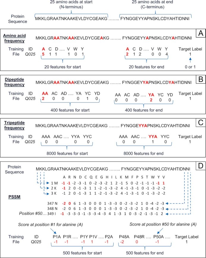
Representation of a protein sequence as a uniform set of features. For illustration, a protein sequence of 349 amino acids (AAs) is represented by a fixed length of numerical features for a machine learning training file using four hypothetical methods (A to D) that can be applied to any sequence length (although 50 AAs is the minimum length in this illustration. That is, only the start (N-terminus) and end (C-terminus) 25 AAs of the sequence are considered here, which are the regions typically known to contain informative signals). In (A) each feature is the frequency of the 20 genetic code AAs in the protein sequence. (B) Each feature is the frequency of a dipeptide–400 possible dipeptide combinations (i.e. 20 AAs raised to the power of two consecutive AAs). (C) Each feature is the frequency of a tripeptide–8000 possible tripeptide combinations (i.e. 20 AAs raised to the power of three consecutive AAs). Methods A to C could theoretically add an additional set of features to represent the varying middle section of a sequence. In such cases, the feature value could be normalized by dividing by the sequence length of the middle. Note that methods A to C do not take into account sequence order. (D) Position-Specific Scoring Matrix (PSSM) is a common format for motifs in biological sequences as an alternative to consensus sequences. There are 20 columns for each genetic code AA and one row for each AA in the protein sequence. Values in the matrix are a normalised (log likelihood) frequency count of each genetic code AA at the same position in a protein multiple sequence alignment e.g. the scores are A = −1, R = −1 etc. for position #1 containing the sequence M (features P1A and P1R) with 500 feature scores in total for the start (i.e. 20 genetic code AAs * 25 sequence positions).

Epidemiology and antimicrobial resistance

Infectious diseases are the leading cause of human mortality worldwide. Microbiology helps explain this epidemiologic reality and holds the potential answers for prevention and treatment. One of the world's foremost healthcare challenges is antimicrobial resistance, which arises when microorganisms evolve to reduce or eliminate the effectiveness of antimicrobial medicines (such as antibiotics and antivirals). Furthermore, emerging pathogens constitute a continuous health threat. Accurate identification and characterization of pathogens, and predicting disease outbreaks are critical steps towards combatting the threat. Identification typically requires cell cultures and light microscopy, which require expertise and can be time consuming. ML with metagenomics and/or image data can automate the identification and characterization process.

Drug-resistant tuberculosis (TB) is a major global public health concern. Rapid, but accurate, identification of this resistance is essential for TB control. Existing rule-based methods identify drug resistance based on the presence of a well-studied single nucleotide polymorphism (SNP). Latest research proposes exploring multivariate association between genetic variants as a more appropriate, although challenging, identification method (Zhang et al. 2013; Walker, Kohl and Omar 2018). One study (Yang et al. 2018) has explored multivariate association with different ML models (including LR, SVM, and RF) to classify drug resistance against eight anti-TB drugs and to classify multi-drug resistance. These models outperformed existing methods in terms of sensitivity to resistance classification. The best model was SVM with data derived from 1839 TB samples. However, as an indication of how ML algorithms perform differently with different training datasets, LR performed best in a similar TB resistance study (Kouchaki et al. 2019) that tested 11 drugs with 13 402 samples collected from 16 countries. In another study (Farhat et al. 2016) with 1397 samples from six reference laboratories, RF performed the best. All three studies highlight that the full complement of mutations encoding resistance to TB drugs is far from established and resistance identification for some drugs is more challenging than others.

The high mutation rate of HIV allows variants to evolve that can be resistant to antiviral drugs. Using ML to predict HIV-drug resistance from viral protein sequences is a potential alternative to an in vitro drug susceptibility test. Except, most ML methods are not able to deal directly with viral sequences containing allele mixtures in at least one position. Furthermore, not all positions on a sequence contribute equally to viral resistance (Iyidogan and Anderson 2014). A study (Ramon, Belanche-Munoz and Perez-Enciso 2019) used a novel approach with weighted SVMs, whereby weighted categorical kernel functions were adapted to take into account the presence of mixtures, and to weigh the different importance of each position (kernels are mathematical functions). A ‘Mean Decrease in Impurity’ metric obtained from RF was used as the weight for position importance. This metric calculates each feature importance as the sum over the number of splits that include the feature, proportionally to the number of samples it splits. It was concluded that resistance prediction may improve when using more sophisticated kernels that also take structural information into account.

One promising new source of data for predicting disease outbreaks is derived from social media such as Twitter and search engines such as Google, which only a decade ago may have seemed ludicrous. Search engines are now practically used daily by most people in the world generating unimaginable volumes of historical searches. The number of searches for a particular keyword in a given timeframe across various regions of the world is referred to as a Keyword Search Volume. Google Trends (https://trends.google.com/trends/?geo=US) is a free website that makes available Keyword Search Volumes. A study from china used a RF model trained on 20 countries to predict the COVID-19 epidemic alert level of next week in 202 countries using Google search volume data (Peng et al. 2020). Data from search engines and social media have also been applied to monitor the outbreak of other infectious diseases (Ginsberg et al. 2009; Shin et al. 2016; Marques-Toledo et al. 2017). Whilst these methods in the latter studies have the capacity for real time tracking of the spread of infectious diseases and a potential to quickly prevent pandemics, they do not currently replace the substantially more accurate traditional surveillance systems using clinical data (albeit a system with days or weeks reporting lag).

Cyclospora cayetanensis causes outbreaks of gastrointestinal illness (Casillas, Bennett and Straily 2018) and has been historically difficult to genotype. This is due to the genetic heterogeneity of the infections it causes, and because it is sometimes difficult to obtain sequence data for all multi-locus-sequence-typing (MLST) loci in a genotyping panel due to various physical limitations (Nascimento et al. 2020). A massive Cyclospora MLST dataset was analysed using an unsupervised ensemble that calculates a dissimilarity metric, even for specimens with missing data and/or possessing multiple haplotypes at their loci (Barratt et al. 2019a) (other dissimilarity measures fall short in various aspects (Plucinski et al. 2015; Barratt et al. 2019a; Jones et al. 2020; Nascimento et al. 2020)). A Bayesian and a heuristic classifier underpin the ensemble (Barratt et al. 2019a) and a performance evaluation using epidemiologically-defined outbreak clusters as ground-truth labels confirmed that it is remarkably sensitive and specific (Nascimento et al. 2020). This ensemble was also applied to a MLST dataset compiled from several genotyping surveys of the human- and dog-infecting worm Strongyloides stercoralis, to detect novel population-level trends (Barratt et al. 2019b). Hierarchical clustering of the resulting distances supported that a sub-population derived mostly from South East Asian dogs is distinct from S. stercoralis infecting humans and might represent a different species (Barratt and Sapp 2020). A subset of S. stercoralis clustering among human-associated genotypes also possessed a propensity towards dogs, supporting the existence of a dog-adapted strain within the human-infecting lineage (Barratt and Sapp 2020).

Antimalarial resistance in Plasmodium falciparum is an increasing problem in Africa where routine antimalarial surveillance is ongoing (Plucinski et al. 2015; Talundzic et al. 2016; Halsey et al. 2017). Assessing antimalarial efficacy involves genotyping malaria parasites when an infection is first identified and treated, followed by genotyping parasites from the same patient if they become ill with malaria again, by sequencing a set of well-defined P. falciparum microsatellite repeats. Comparison of microsatellite profiles before and after treatment enables assessment of whether patients remained infected with the original strain due to a treatment failure, or if they are infected with a new strain (Plucinski et al. 2015). An unsupervised Bayesian classifier was developed to classify malaria cases as a recrudescence (treatment failure) or reinfection based on their microsatellite profiles, given that manual interpretation of these profiles can be challenging and subject to bias (Slater et al. 2005). An evaluation of this approach on simulated datasets supported that manually performed human classification of microsatellite profiles could lead to gross under- or over-estimation of drug efficacy, while the Bayesian approach was highly specific and provided an accurate assessment of treatment failure rates (Jones et al. 2020).

Streptococcus pneumoniae colonizes the nasopharynx of healthy individuals though may disseminate in a compromised immune system (Mitchell and Mitchell 2010). The S. pneumoniae polysaccharide capsule is a major cell surface structure, and differentiation of capsular serotypes is important for molecular surveillance (Gonzales-Siles et al. 2019). Traditionally, the Quellung reaction is used to differentiate serotypes, involving a reaction between antibody and its specific capsular polysaccharide motifs, causing cells to swell; a microscopically visible process. This test is relatively expensive and is typically restricted to reference laboratories (Burckhardt et al. 2019). A database of fourier-transformed infrared (FT-IR) spectra generated from a variety of known strains was hierarchically clustered alongside spectra generated for sets of invasive and non-invasive strains, and several uncharacterised types. Clusters identified were compared to the results of the Quellung reaction (ground truth labels) to assess the robustness of hierarchical clustering (unsupervised classification) using the Euclidean—average—mean spectra algorithm. Excellent concordance between the Quellung reaction and clustering based on FT-IR spectra was observed (Burckhardt et al. 2019).

Microbial ecology and microbiomes

The central focus of microbial ecology is to understand interactions of microorganisms with one another and with their environment, which has enormous implications for all life on this planet. Advances in genome sequencing technologies and metagenomics have seen an upsurge in research of microorganisms and their genomes (collectively called the microbiome), which is increasingly linked to many aspects of human health and disease.

Microbial DNA and RNA are found in human tissues and blood, including within or around tumour cells (Robinson et al. 2017). A study (Poore et al. 2020) using stochastic gradient-boosting ML models (an additive regression method) (Friedman 2002) examined whether microbial community structure and dynamics (i.e. microbial signatures) could be cancer predictors. Source data were derived from The Cancer Genome Atlas (TCGA) (Weinstein et al. 2013) online resource and processed by Kraken (assigns taxonomic labels to metagenomic DNA sequences) (Wood and Salzberg 2014), Voom (transforms RNA-Seq data ready for linear modelling) (Law et al. 2014) and SNM R package (performs supervised normalisation) (Mecham, Nelson and Storey 2010). The processed data prior to training comprised ‘normalised read counts at the genus taxonomic level’ representing 17 625 samples, 10 183 patients and 32 cancer types sourced from TCGA. Overall, the models performed well in discriminating between cancer types and between cancer and normal tissue (suggesting microbial signatures are unique to each cancer type), but less well when discriminating between different stages of the same cancer type (suggesting microbial signatures may not correlate with cancer stages for all cancer types) (Poore et al. 2020). Importantly, the proposed ML strategy has potential to be a microbiome-based cancer diagnostic tool.

Merging published microbial data is a potential opportunity to address global-scale questions such as predicting the response of soil organisms to global environmental change (Garcia-Palacios et al. 2015). Furthermore, variation in microbial community structure is possibly more ecologically relevant than measures of diversity and abundances of major taxa (Ramirez et al. 2018). Community structure is largely defined by the relative abundances of individual taxa. One difficulty is that microbial community data are mainly disseminated in disparate published studies with inherent biases (e.g. different sampling and sequencing methodologies). Applying RF to global soil microbial community patterns from merged independent taxonomy-based datasets was assessed (Ramirez et al. 2018). Despite biases between studies, many bacterial taxa are still informative when assessing community structure. Rare bacterial taxa were more important than abundant taxa in differentiating communities.

Different organisms in a microbial community affect each other's growth to form complex networks of interdependencies. These ecosystem networks govern a community's functional properties and dynamics. Significant network changes have important implications for human and environmental health. Measuring pairwise interactions in coculture experiments is a historically accepted method to interpret ecosystem networks. However, performing the experiments for all possible pairwise interactions given the huge diversity of many natural communities is deemed an almost insurmountable task (DiMucci, Kon and Segre 2018). A study (DiMucci, Kon and Segre 2018) demonstrated a proof of principle using RF to predict microbial interactions given trait descriptions (features) for each community organism. RF was chosen because it required no a priori assumptions about the underlying relationships between community members, and provided ‘feature contribution’ metrics. Three communities, where all pairwise experiments had been performed and interactions observed, were used for ML training and verification. The presence or absence of a trait was encoded in one binary vector per organism. To represent every possible pairwise interaction, a composite vector was created by concatenating corresponding organism vectors. Observed interactions were labelled accordingly (i.e. target label defined) and these concatenated vectors were then used to train a model that predicted the outcome of unobserved interactions. RF feature contributions were proposed as a way to develop new hypotheses about the mechanisms that mediate specific interactions (DiMucci, Kon and Segre 2018).

Analysing the post-mortem microbiome has the potential to provide valuable information to forensic science and general death investigations. Furthermore, post-mortem microbiome data can potentially help explain ante-mortem health, which could be used for public health diagnosis. This potential has been slow to be fulfilled because the computational requirements and best practices to extract the full value from microbial datasets have yet to be determined. A study (Zhang et al. 2019) tested the abilities of three ML algorithms (RF, ANN and boosted algorithms) to predict death investigation attributes (e.g. time, location of death) given post-mortem microbial data from 188 death investigations. Different ML models were created using various combinations and selections from 100 features, which included metadata categories (e.g. sex, race, age, death location) and microbial taxonomic information (determined from rRNA gene amplicon sequencing). The results support the principle of having in the future a molecular autopsy and ML approach for routine death investigations and clinical diagnostics (Zhang et al. 2019).

Ordination methods (i.e. dimensionality reduction procedures) are widely used to distinguish microbial communities based on bacterial 16S sequence composition (Hawinkel et al. 2019). However, some ordination methods often do not account for dispersion effects and high-statistical sparsity, which are inherent in microbiome datasets. Furthermore, failure to detect taxa (resulting in a zero count for that taxon) may represent a true absence or an undetected presence, though is considered a true absence by many ordination methods. A novel ordination approach referred to as GLM (generalized linear model)-based Ordination Method for Microbiome Samples (GOMMS) that accounts for these problems during dimensionality reduction was evaluated on 16S datasets generated from the human nasopharynx and oropharynx (Sohn and Li 2018). The GOMMS procedure was compared to distance-based ordination procedures applied to the same datasets, confirming that GOMMS performed well on datasets that suffered from dispersion effects while the other methods displayed clear problems on the effected datasets (Sohn and Li 2018).

CONCLUDING REMARKS

Machine learning is rapidly being incorporated in almost every research area. It is perhaps no longer possible to even quantify the increasing multitudes of ML applications. ML importance to microbiology is exemplified by escalating applications to the greatest global health crisis of our age, the coronavirus COVID-19 pandemic. As of January 2021, 607 papers focusing on ‘COVID-19’ and ‘machine learning’ have been published (source: PubMed search engine), covering research areas such as vaccine design (Ong et al. 2020), diagnosis (Albahri et al. 2020; Brinati et al. 2020; Elaziz et al. 2020; Khuzani, Heidari and Shariati 2020), drug repurposing (Gao et al. 2020; Mirabelli et al. 2020), and epidemiology (Mackey et al. 2020; Santosh 2020; Yang et al. 2020). The aim of this review was to inspire those microbiologists and other related researchers that have yet to fully appreciate the enormous potential of ML. To understand the intricacies of microorganisms at the molecular level requires making sense of copious volumes of data; so much data that it may in the near future be humanly impossible to detect crucial insightful data patterns that may answer the important questions without ML or other computational techniques.

We described the most pertinent concepts for ML followed by real life examples of how ML can assist in microbiology. These examples demonstrate some of the types of problems that can be addressed but are by no means exhaustive (additional examples are listed in Table 1 of Supporting information 1). Machine learning can be applied to any problem with appropriate data. The appropriate data ingredient here with respect to performing supervised classification is rows of features/predictors with known classifications (i.e. training data). It may not always be clear to a human whether there is any relationship between the features and the classification. Happily, this is not a prerequisite to using ML. Hence the important point here, for a researcher contemplating whether ML is a worthwhile endeavour for their particular data, is to first establish the feasibility of creating a training dataset and then let the performance evaluation determine whether it is worthwhile or not.

Challenges remain with the use of ML in microbiology. Whilst the reviewed ML algorithms function exceptionally well given sufficient quality training data as substantially supported in the literature, obtaining the quality training data remains a challenge. Furthermore, data is rarely perfect irrespective of the source, which may introduce noise. Mitigating against noisy and inconsistent data, through data cleaning and/or the use of normalisation to repair variation in genomic and flow cytometry data across technology platforms requires time and effort. Some kinds of datasets are challenging for ML. In particular, it is very challenging to build ML models that generalise on highly dimensional data with relatively few instances and that are unbalanced with respect to the values of the target attribute. Unfortunately, many data of interest fit these criteria; including genomics, flow cytometry, image and text data. Heavily regularised models, feature extraction or fine-tuning of pre-trained deep neural networks can help with these problems. Validation of predictions from ML is challenging. Predictions from biological data may remain unverified until laboratory experiments can be performed. The best compromise is effective validation of models to indicate their expected performance on unseen data, with the assumption that the training data is representative. Notwithstanding the current work in Explainable AI (XAI), it can be challenging to understand the train of logic for how black box ML algorithms arrive at a prediction or to characterise a derived clustering, particularly in high dimensional settings. This may make it difficult for users to trust predictions. Not least of all there are challenges inherent in multidisciplinary research. Long term collaborations are required for researchers to learn to communicate and embrace data-sharing.

Despite these challenges, ML has a rosy future in microbiology. As algorithms become more mature and trusted they will become parts of workflows (e.g. in Galaxy or Bioconductor) making them accessible to researchers. State of the art ML algorithms, especially deep learning neural networks, can deal with mammoth datasets of images, text (e.g. PubMed articles or genome/experimental annotations) and strings (such as genomic sequences). Internet databases are full of these kinds of data, which have previously been too difficult to use. There is a golden opportunity to combine data from disparate sources and solve problems that have previously been intractable.

A microbiologist in our opinion has two options: to embrace the ML revolution and start the journey of becoming an effective ML practitioner or accept that ML is some abstruse art better left to mathematicians and computer scientists.

Disclaimer

The views and opinions in this report are those of the authors and do not necessarily represent the official position of the Centers for Disease Control and Prevention/the Agency for Toxic Substances and Disease Registry.

REFERENCES

- Ahmed WM, Bayraktar B, Bhunia AKet al. Classification of bacterial contamination using image processing and distributed computing. IEEE J Biomed Health Inform. 2013;17:232–9. [DOI] [PubMed] [Google Scholar]
- Albahri AS, Hamid RA, Alwan JKet al. Role of biological Data Mining and Machine Learning Techniques in Detecting and Diagnosing the Novel Coronavirus (COVID-19): a systematic review. J Med Syst. 2020;44:122. [DOI] [PMC free article] [PubMed] [Google Scholar]
- Ates H, Gerek ON, Ieee. An Image-Processing Based Automated Bacteria Colony Counter. 2009. [Google Scholar]
- Barratt JLN, Lane M, Talundzic Eet al. A global genotyping survey of Strongyloides stercoralis and Strongyloides fuelleborni using deep amplicon sequencing. PLoS Negl Trop Dis. 2019b;13:e0007609. [DOI] [PMC free article] [PubMed] [Google Scholar]
- Barratt JLN, Park S, Nascimento FSet al. Genotyping genetically heterogeneous Cyclospora cayetanensis infections to complement epidemiological case linkage. Parasitology. 2019a;146:1275–83. [DOI] [PMC free article] [PubMed] [Google Scholar]
- Barratt JLN, Sapp SGH. Machine learning-based analyses support the existence of species complexes for Strongyloides fuelleborni and Strongyloides stercoralis. Parasitology. 2020;1–46. [DOI] [PMC free article] [PubMed] [Google Scholar]
- Becht E, McInnes L, Healy Jet al. Dimensionality reduction for visualizing single-cell data using UMAP. Nat Biotechnol. 2019;37:38–+. [DOI] [PubMed] [Google Scholar]
- Bibin D, Nair MS, Punitha P. Malaria parasite detection from peripheral blood smear images using deep belief networks. IEEE Access. 2017;5:9099–108. [Google Scholar]
- Bray JR, Curtis JT. An ordination of the upland forest communities of Southern Wisconsin. Ecological Monographs. 1957;27:326–49. [Google Scholar]
- Brinati D, Campagner A, Ferrari Det al. Detection of COVID-19 Infection from Routine Blood Exams with Machine Learning: a Feasibility Study. J Med Syst. 2020;44:135. [DOI] [PMC free article] [PubMed] [Google Scholar]
- Burckhardt I, Sebastian K, Mauder Net al. Analysis of Streptococcus pneumoniae using Fourier-transformed infrared spectroscopy allows prediction of capsular serotype. Eur J Clin Microbiol Infect Dis. 2019;38:1883–90. [DOI] [PMC free article] [PubMed] [Google Scholar]
- Casillas SM, Bennett C, Straily A. Notes from the field: multiple Cyclosporiasis Outbreaks - United States, 2018. MMWR Morb Mortal Wkly Rep. 2018;67:1101–2. [DOI] [PMC free article] [PubMed] [Google Scholar]
- Cieslak MC, Castelfranco AM, Roncalli Vet al. t-Distributed Stochastic Neighbor Embedding (t-SNE): a tool for eco-physiological transcriptomic analysis. Mar Genomics. 2020;51:100723. [DOI] [PubMed] [Google Scholar]
- Colubri A, Silver T, Fradet Tet al. Transforming Clinical Data into Actionable Prognosis Models: machine-Learning Framework and Field-Deployable App to Predict Outcome of Ebola Patients. PLoS Negl Trop Dis. 2016;10. [DOI] [PMC free article] [PubMed] [Google Scholar]
- De Bruyne K, Slabbinck B, Waegeman Wet al. Bacterial species identification from MALDI-TOF mass spectra through data analysis and machine learning. Syst Appl Microbiol. 2011;34:20–29. [DOI] [PubMed] [Google Scholar]
- Diederich B, Wartmann R, Schadwinkel Het al. Using machine-learning to optimize phase contrast in a low-cost cellphone microscope. PLoS One. 2018;13. [DOI] [PMC free article] [PubMed] [Google Scholar]
- DiMucci D, Kon M, Segre D. Machine Learning Reveals Missing Edges and Putative Interaction Mechanisms in Microbial Ecosystem Networks. Msystems. 2018;3. [DOI] [PMC free article] [PubMed] [Google Scholar]
- Dong Y, Jiang Z, Shen Het al. Evaluations of Deep Convolutional Neural Networks for Automatic Identification of Malaria Infected Cells. Orlando, FL, USA: 2017 IEEE EMBS International Conference on Biomedical & Health Informatics (BHI), 2017. [Google Scholar]
- Elaziz MA, Hosny KM, Salah Aet al. New machine learning method for image-based diagnosis of COVID-19. PLoS One. 2020;15:e0235187. [DOI] [PMC free article] [PubMed] [Google Scholar]
- Farhat MR, Sultana R, Iartchouk Oet al. Genetic Determinants of Drug Resistance in Mycobacterium tuberculosis and Their Diagnostic Value. Am J Respir Crit Care Med. 2016;194:621–30. [DOI] [PMC free article] [PubMed] [Google Scholar]
- Flach P. Machine Learning: The Art and Science of Algorithms that Make Sense of Data. Cambridge: Cambridge University Press, 2012. [Google Scholar]
- Fong RC, Vedaldi A, Ieee. Interpretable Explanations of Black Boxes by Meaningful Perturbation. 2017 IEEE International Conference on Computer Vision, 2017, 3449–57. [Google Scholar]
- Forero MG, Cristobal G, Desco M. Automatic identification of Mycobacterium tuberculosis by Gaussian mixture models. J Microsc. 2006;223:120–32. [DOI] [PubMed] [Google Scholar]
- Friedman JH. Stochastic gradient boosting. Computational Statistics, Data Analysis. 2002;38:367–78. [Google Scholar]
- G. Howard A, Zhu M, Chen Bet al. MobileNets: Efficient Convolutional Neural Networks for Mobile Vision Applications. Preprint at https://arxiv.org/abs/1704.04861, 2017. [Google Scholar]
- Gao K, Nguyen DD, Chen Jet al. Repositioning of 8565 Existing Drugs for COVID-19. J Phys Chem Lett. 2020;11:5373–82. [DOI] [PMC free article] [PubMed] [Google Scholar]
- GarcÃa-Palacios P, Vandegehuchte ML, Shaw EAet al. Are there links between responses of soil microbes and ecosystem functioning to elevated CO2, N deposition and warming? A global perspective. Global Change Biol. 2015;21:1590–600. [DOI] [PubMed] [Google Scholar]
- Gardner WA. Learning characteristics of stochastic-gradient-descent algorithms - a general study, analysis, and critique. Signal Process. 1984;6:113–33. [Google Scholar]
- Ginsberg J, Mohebbi MH, Patel RSet al. Detecting influenza epidemics using search engine query data. Nature. 2009;457:1012–U1014. [DOI] [PubMed] [Google Scholar]
- Gonzales-Siles L, Salva-Serra F, Degerman Aet al. Identification and capsular serotype sequetyping of Streptococcus pneumoniae strains. J Med Microbiol. 2019;68:1173–88. [DOI] [PubMed] [Google Scholar]
- Goodswen SJ, Kennedy PJ, Ellis JT. A novel strategy for classifying the output from an in silico vaccine discovery pipeline for eukaryotic pathogens using machine learning algorithms. BMC Bioinformatics. 2013;14. [DOI] [PMC free article] [PubMed] [Google Scholar]
- Goodswen SJ, Kennedy PJ, Ellis JT. Vacceed: a high-throughput in silico vaccine candidate discovery pipeline for eukaryotic pathogens based on reverse vaccinology. Bioinformatics. 2014;30:2381–3. [DOI] [PMC free article] [PubMed] [Google Scholar]
- Guidotti R, Monreale A, Ruggieri Set al. A Survey of Methods for Explaining Black Box Models. ACM Computing Surveys. 2019;51. [Google Scholar]
- Halkidi M, Batistakis Y, Vazirgiannis M. On clustering validation techniques. J Intelligent Inform Syst. 2001;17:107–45. [Google Scholar]
- Halsey ES, Venkatesan M, Plucinski MMet al. Capacity Development through the US President's Malaria Initiative-Supported Antimalarial Resistance Monitoring in Africa Network. Emerg Infect Dis. 2017;23. [DOI] [PMC free article] [PubMed] [Google Scholar]
- Handelman GS, Kok HK, Chandra RVet al. Peering Into the Black Box of Artificial Intelligence: evaluation Metrics of Machine Learning Methods. Am J Roentgenol. 2019;212:38–43. [DOI] [PubMed] [Google Scholar]
- Hawinkel S, Kerckhof F-M, Bijnens Let al. A unified framework for unconstrained and constrained ordination of microbiome read count data. PLoS One. 2019;14. [DOI] [PMC free article] [PubMed] [Google Scholar]
- He H, Garcia EA. Learning from Imbalanced Data. IEEE Trans Knowl Data Eng. 2009;21:1263–84. [Google Scholar]
- Hipp J, Güntzer U, Nakhaeizadeh G. Algorithms for association rule mining — a general survey and comparison. ACM SIGKDD Explorations Newsletter. 2000;2:58–64. [Google Scholar]
- Holsinger KE, Weir BS. Genetics in geographically structured populations: defining, estimating and interpreting F-ST. Nat Rev Genet. 2009;10:639–50. [DOI] [PMC free article] [PubMed] [Google Scholar]
- Huang X, Wu L, Ye Y. A Review on Dimensionality Reduction Techniques. Int J Pattern Recognit Artif Intell. 2019;33. [Google Scholar]
- Iyidogan P, Anderson KS. Current Perspectives on HIV-1 Antiretroviral Drug Resistance. Viruses-Basel. 2014;6:4095–139. [DOI] [PMC free article] [PubMed] [Google Scholar]
- Jaccard P. The Distribution of the Flora of the Alpine Zone. New Phytol. 1912;11:37–50. [Google Scholar]
- James G, Witten D, Hastie Tet al. An Introduction to Statistical Learning with Applications in R Introduction. New York: Springer, 2013. [Google Scholar]
- Jones S, Plucinski M, Kay Ket al. A Computer Modelling Approach To Evaluate the Accuracy of Microsatellite Markers for Classification of Recurrent Infections during Routine Monitoring of Antimalarial Drug Efficacy. Antimicrob Agents Chemother. 2020;64. [DOI] [PMC free article] [PubMed] [Google Scholar]
- Khuzani AZ, Heidari M, Shariati SA. COVID-Classifier: an automated machine learning model to assist in the diagnosis of COVID-19 infection in chest x-ray images. medRxiv. 2020. [DOI] [PMC free article] [PubMed] [Google Scholar]
- Kouchaki S, Yang Y, Walker TMet al. Application of machine learning techniques to tuberculosis drug resistance analysis. Bioinformatics. 2019;35:2276–82. [DOI] [PMC free article] [PubMed] [Google Scholar]
- Law CW, Chen Y, Shi Wet al. voom: precision weights unlock linear model analysis tools for RNA-seq read counts. Genome Biol. 2014;15. [DOI] [PMC free article] [PubMed] [Google Scholar]
- Liang Z, Powell A, Ersoy Iet al. CNN-Based Image Analysis for Malaria Diagnosis. Shenzhen, China: 2016 IEEE International Conference on Bioinformatics and Biomedicine (BIBM), 2016, 493–6. [Google Scholar]
- London AJ. Artificial Intelligence and Black-Box Medical Decisions: accuracy versus Explainability. Hastings Cent Rep. 2019;49:15–21. [DOI] [PubMed] [Google Scholar]
- Mackey T, Purushothaman V, Li Jet al. Machine Learning to Detect Self-Reporting of Symptoms, Testing Access, and Recovery Associated With COVID-19 on Twitter: retrospective Big Data Infoveillance Study. JMIR Public Health Surveill. 2020;6:e19509. [DOI] [PMC free article] [PubMed] [Google Scholar]
- Marques-Toledo CdA, Degener CM, Vinhal Let al. Dengue prediction by the web: tweets are a useful tool for estimating and forecasting Dengue at country and city level. PLoS NeglTrop Dis. 2017;11. [DOI] [PMC free article] [PubMed] [Google Scholar]
- Mathison BA, Kohan JL, Walker JFet al. Detection of Intestinal Protozoa in Trichrome-Stained Stool Specimens by Use of a Deep Convolutional Neural Network. J Clin Microbiol. 2020;58. [DOI] [PMC free article] [PubMed] [Google Scholar]
- McInnes L, Healy J. UMAP: uniform manifold approximation and projection for dimension reduction. Preprint at https://arxiv.org/abs/1802.03426, 2018.
- Mecham BH, Nelson PS, Storey JD. Supervised normalization of microarrays. Bioinformatics. 2010;26:1308–15. [DOI] [PMC free article] [PubMed] [Google Scholar]
- Meites E, Gaydos CA, Hobbs MMet al. A Review of Evidence-Based Care of Symptomatic Trichomoniasis and Asymptomatic Trichomonas vaginalis Infections. Clin Infect Dis. 2015;61:S837–48. [DOI] [PMC free article] [PubMed] [Google Scholar]
- Mirabelli C, Wotring JW, Zhang CJet al. Morphological Cell Profiling of SARS-CoV-2 Infection Identifies Drug Repurposing Candidates for COVID-19. bioRxiv. 2020. [DOI] [PMC free article] [PubMed] [Google Scholar]
- Mitchell AM, Mitchell TJ. Streptococcus pneumoniae: virulence factors and variation. Clin Microbiol Infect. 2010;16:411–8. [DOI] [PubMed] [Google Scholar]
- Mitchell TM. Machine Learning. New York: McGraw-Hill, 1997. [Google Scholar]
- Nascimento FS, Barratt J, Houghton Ket al. Evaluation of an ensemble-based distance statistic for clustering MLST datasets using epidemiologically defined clusters of cyclosporiasis. Epidemiol Infect. under peer review2020. [DOI] [PMC free article] [PubMed] [Google Scholar]
- Nei M. Genetic Distance between Populations. Am Nat. 1972;106:283–+. [Google Scholar]
- Ong DSY, Poljak M. Smartphones as mobile microbiological laboratories. Clin Microbiol Infect. 2019. [DOI] [PubMed] [Google Scholar]
- Ong E, Wong MU, Huffman Aet al. COVID-19 coronavirus vaccine design using reverse vaccinology and machine learning. bioRxiv. 2020. [DOI] [PMC free article] [PubMed] [Google Scholar]
- Peng Y, Li C, Rong Yet al. Retrospective analysis of the accuracy of predicting the alert level of COVID-19 in 202 countries using Google Trends and machine learning. Journal of global health. 2020;10:020511–. [DOI] [PMC free article] [PubMed] [Google Scholar]
- Pirnstill CW, Cote GL. Malaria Diagnosis Using a Mobile Phone Polarized Microscope. Sci Rep. 2015;5. [DOI] [PMC free article] [PubMed] [Google Scholar]
- Plucinski MM, Morton L, Bushman Met al. Robust Algorithm for Systematic Classification of Malaria Late Treatment Failures as Recrudescence or Reinfection Using Microsatellite Genotyping. Antimicrob Agents Chemother. 2015;59:6096–100. [DOI] [PMC free article] [PubMed] [Google Scholar]
- Poore GD, Kopylova E, Zhu Qet al. Microbiome analyses of blood and tissues suggest cancer diagnostic approach. Nature. 2020;579:567–+. [DOI] [PMC free article] [PubMed] [Google Scholar] [Retracted]
- Poostchi M, Silamut K, Maude RJet al. Image analysis and machine learning for detecting malaria. Translational Research. 2018;194:36–55. [DOI] [PMC free article] [PubMed] [Google Scholar]
- Pérez-Suárez A, Martinez-Trinidad JF, Carrasco-Ochoa JA. A review of conceptual clustering algorithms. Artificial Intelligence Review. 2019;52:1267–96. [Google Scholar]
- Rahman MS, Rahman MK, Saha Set al. Antigenic: an improved prediction model of protective antigens. Artificial Intelligence in Medicine. 2019;94:28–41. [DOI] [PubMed] [Google Scholar]
- Rajaraman S, Antani SK, Poostchi Met al. Pre-trained convolutional neural networks as feature extractors toward improved malaria parasite detection in thin blood smear images. Peerj. 2018;6. [DOI] [PMC free article] [PubMed] [Google Scholar]
- Ramirez KS, Knight CG, de Hollander Met al. Detecting macroecological patterns in bacterial communities across independent studies of global soils. Nature Microbiology. 2018;3:189–96. [DOI] [PubMed] [Google Scholar]
- Ramon E, Belanche-Munoz L, Perez-Enciso M. HIV drug resistance prediction with weighted categorical kernel functions. BMC Bioinformatics. 2019;20. [DOI] [PMC free article] [PubMed] [Google Scholar]
- Ribeiro MT, Singh S, Guestrin Cet al. “Why Should I Trust You?” Explaining the Predictions of Any Classifier. Preprint at https://arxiv.org/abs/1602.04938, 2016. [Google Scholar]
- Robinson KM, Crabtree J, Mattick JSAet al. Distinguishing potential bacteria-tumor associations from contamination in a secondary data analysis of public cancer genome sequence data. Microbiome. 2017;5. [DOI] [PMC free article] [PubMed] [Google Scholar]
- Rokach L. A survey of Clustering Algorithms. Data Mining and Knowledge Discovery Handbook, 2009, 269–98. [Google Scholar]
- Ross NE, Pritchard CJ, Rubin DMet al. Automated image processing method for the diagnosis and classification of malaria on thin blood smears. Med, Bio Engineering, Comp. 2006;44:427–36. [DOI] [PubMed] [Google Scholar]
- Rousseeuw PJ. Silhouettes - a graphical aid to the interpretation and validation of cluster-analysis. J Comput Appl Math. 1987;20:53–65. [Google Scholar]
- Saito T, Rehmsmeier M. The Precision-Recall Plot Is More Informative than the ROC Plot When Evaluating Binary Classifiers on Imbalanced Datasets. PLoS One. 2015;10. [DOI] [PMC free article] [PubMed] [Google Scholar]
- Santosh KC. AI-Driven Tools for Coronavirus Outbreak: need of Active Learning and Cross-Population Train/Test Models on Multitudinal/Multimodal Data. J Med Syst. 2020;44. [DOI] [PMC free article] [PubMed] [Google Scholar]
- Saxena A, Prasad M, Gupta Aet al. A review of clustering techniques and developments. Neurocomputing. 2017;267:664–81. [Google Scholar]
- Shin S-Y, Seo D-W, An Jet al. High correlation of Middle East respiratory syndrome spread with Google search and Twitter trends in Korea. Sci Rep. 2016;6. [DOI] [PMC free article] [PubMed] [Google Scholar]
- Slater M, Kiggundu M, Dokomajilar Cet al. Distinguishing recrudescences from new infections in antimalarial clinical trials: major impact of interpretation of genotyping results on estimates of drug efficacy. Am J Trop Med Hyg. 2005;73:256–62. [PubMed] [Google Scholar]
- Sohn MB, Li H. A GLM-based latent variable ordination method for microbiome samples. Biometrics. 2018;74:448–57. [DOI] [PMC free article] [PubMed] [Google Scholar]
- Sommer C, Gerlich DW. Machine learning in cell biology - teaching computers to recognize phenotypes. J Cell Sci. 2013;126:5529–39. [DOI] [PubMed] [Google Scholar]
- Svarovskaia ES, Cheslock SR, Zhang WHet al. Retroviral mutation rates and reverse transcriptase fidelity. Front Bioscience-Landmark. 2003;8:D117–34. [DOI] [PubMed] [Google Scholar]
- Talundzic E, Plucinski MM, Biliya Set al. Advanced Molecular Detection of Malarone Resistance. Antimicrob Agents Chemother. 2016;60:3821–3. [DOI] [PMC free article] [PubMed] [Google Scholar]
- Vamathevan J, Clark D, Czodrowski Pet al. Applications of machine learning in drug discovery and development. Nat Rev Drug Discovery. 2019;18:463–77. [DOI] [PMC free article] [PubMed] [Google Scholar]
- van der Maaten L, Hinton G. Visualizing Data using t-SNE. J Machine Learning Res. 2008;9:2579–605. [Google Scholar]
- Velliangiri S, Alagumuthukrishnan S, Joseph SIT. A Review of Dimensionality Reduction Techniques for Efficient Computation. In: Nithyanandam P, Parvathi R, Kannan RJ, Khan AN (eds). 2nd International Conference on Recent Trends in Advanced Computing Icrtac -Disrup - Tiv Innovation, 2019. Procedia Computer Science; , 2019;165::104–11. [Google Scholar]
- Verma R, Tiwari A, Kaur Set al. Identification of proteins secreted by malaria parasite into erythrocyte using SVM and PSSM profiles. BMC Bioinformatics. 2008;9. [DOI] [PMC free article] [PubMed] [Google Scholar]
- Walker TM, Kohl TA, Omar SV. Whole-genome sequencing for prediction of Mycobacterium tuberculosis drug susceptibility and resistance: a retrospective cohort study (vol 15, pg 1193, 2015). Lancet Infectious Diseases. 2018;18:21–1. [DOI] [PMC free article] [PubMed] [Google Scholar]
- Wang HY, Hung CC, Chen CHet al. Increase Trichomonas vaginalis detection based on urine routine analysis through a machine learning approach. Sci Rep. 2019;9. [DOI] [PMC free article] [PubMed] [Google Scholar]
- Weinstein JN, Collisson EA, Mills GBet al. The Cancer Genome Atlas Pan-Cancer analysis project. Nat Genet. 2013;45:1113–20. [DOI] [PMC free article] [PubMed] [Google Scholar]
- Williams GJ. Rattle: a Data Mining GUI for R. R J. 2009;1:45–55. [Google Scholar]
- Wood DE, Salzberg SL. Kraken: ultrafast metagenomic sequence classification using exact alignments. Genome Biol. 2014;15. [DOI] [PMC free article] [PubMed] [Google Scholar]
- Xu D, Tian Y. A Comprehensive Survey of Clustering Algorithms. Ann Data Sci. 2015;2:165–93. [Google Scholar]
- Xu X, Liang T, Zhu Jet al. Review of classical dimensionality reduction and sample selection methods for large-scale data processing. Neurocomputing. 2019;328:5–15. [Google Scholar]
- Yang Y, Niehaus KE, Walker TMet al. Machine learning for classifying tuberculosis drug-resistance from DNA sequencing data. Bioinformatics. 2018;34:1666–71. [DOI] [PMC free article] [PubMed] [Google Scholar]
- Yang ZF, Zeng ZQ, Wang Ket al. Modified SEIR and AI prediction of the epidemics trend of COVID-19 in China under public health interventions. J Thoracic Dis. 2020;12:165–+. [DOI] [PMC free article] [PubMed] [Google Scholar]
- Zeiler MD, Fergus R. Visualizing and Understanding Convolutional Networks. In: Fleet D, Pajdla T, Schiele B, Tuytelaars T (eds). Computer Vision – ECCV, 689:Lecture Notes in Computer Science. Cham: Springer, 2014. [Google Scholar]
- Zhang HT, Li DF, Zhao LLet al. Genome sequencing of 161 Mycobacterium tuberculosis isolates from China identifies genes and intergenic regions associated with drug resistance. Nat Genet. 2013;45:1255–U1217. [DOI] [PubMed] [Google Scholar]
- Zhang Y, Pechal JL, Schmidt CJet al. Machine learning performance in a microbial molecular autopsy context: a cross-sectional postmortem human population study. PLoS One. 2019;14. [DOI] [PMC free article] [PubMed] [Google Scholar]
- Zielinski B, Plichta A, Misztal Ket al. Deep learning approach to bacterial colony classification. PLoS One. 2017;12. [DOI] [PMC free article] [PubMed] [Google Scholar]
- Zorn KM, Lane TR, Russo DPet al. Multiple Machine Learning Comparisons of HIV Cell-based and Reverse Transcriptase Data Sets. Mol Pharm. 2019;16:1620–32. [DOI] [PMC free article] [PubMed] [Google Scholar]
Associated Data
This section collects any data citations, data availability statements, or supplementary materials included in this article.