Abstract
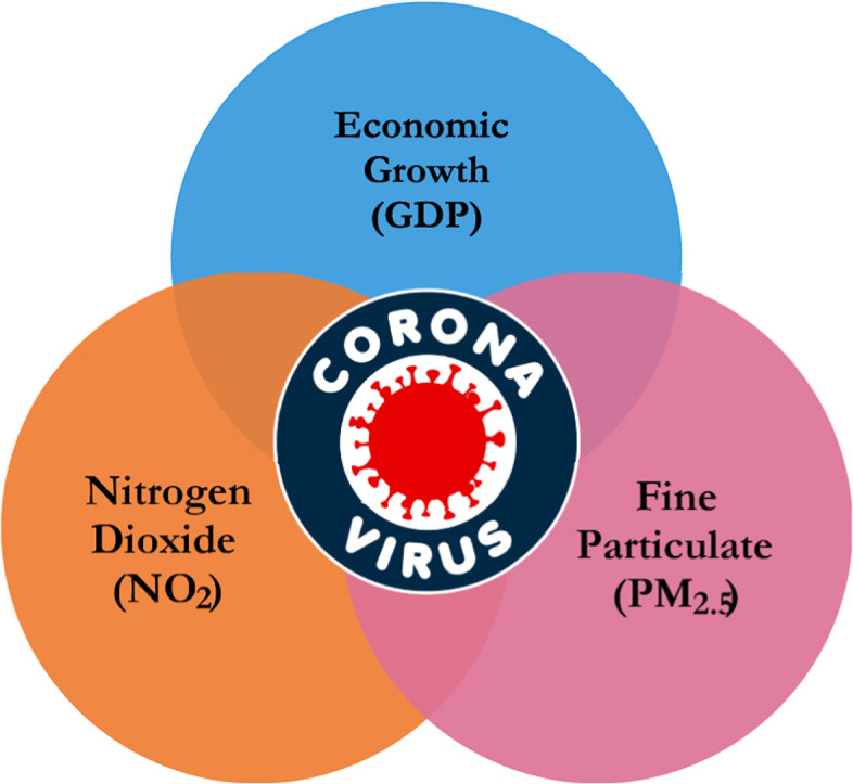
The aim of this paper is to assess the relationship between COVID-19-related deaths, economic growth, PM10, PM2.5, and NO2 concentrations in New York state using city-level daily data through two Machine Learning experiments. PM2.5 and NO2 are the most significant pollutant agents responsible for facilitating COVID-19 attributed death rates. Besides, we found only six out of many tested causal inferences to be significant and true within the AUPRC analysis. In line with the causal findings, a unidirectional causal effect is found from PM2.5 to Deaths, NO2 to Deaths, and economic growth to both PM2.5 and NO2. Corroborating the first experiment, the causal results confirmed the capability of polluting variables (PM2.5 to Deaths, NO2 to Deaths) to accelerate COVID-19 deaths. In contrast, we found evidence that unsustainable economic growth predicts the dynamics of air pollutants. This shows how unsustainable economic growth could increase environmental pollution by escalating emissions of pollutant agents (PM2.5 and NO2) in New York state.
Keywords: COVID-19, Air pollution, Economic growth, New York state, Machine learning
Graphical abstract
1. Introduction
The viral pandemic caused by SARS-CoV-2 has raised numerous questions regarding the role played by environmental pollution in the spread of the virus (Sarkodie and Owusu, 2020a,b). In particular, extensive scientific literature connects cases of viral infection with concentrations of atmospheric Particulate Matter (PM10 and PM2.5) (Ciencewicki et al., 2007; Sedlmaier et al., 2009; Perrino et al., 2014; Mele and Magazzino, 2020; Sterpetti, 2020). In general, the correlation between the spread of a virus and PM10 and PM2.5 levels passes through direct and indirect effects. Concerning the first, the atmospheric particulate would play the role of transport vector (Chen et al., 2010; Despres et al., 2012; Cao et al., 2014; Lei et al., 2018; Magazzino et al., 2020). Regarding indirect effects, prolonged inhalation of fine and ultrafine particulates would induce oxidative stress and cellular inflammation of the lungs, which would assist the adverse effects of respiratory viruses (COVID-19) on patients (Bengalli et al., 2019; Esquivel-Fariña et al., 2019; Li et al., 2020; Putrino et al., 2020). These results have led numerous international and academic research centers to more precisely analyze the role of high concentrations of PM10 and PM2.5 in the spread, morbidity, and mortality attributable to the pandemic COVID-19 virus (Dominici et al., 2020; Magazzino et al., 2020a, b, c, d; Mahase, 2020; Remuzzi et al., 2020). The connection between pollution and the possible spread of viruses and new pandemics passes through the unsustainable economic growth process. In this situation, there is the case of the U.S. which continues to weaken the standards of environmental protection to promote more significant economic growth (Environmental Protection Agency, 2019). The correlation between environmental performance and growth in the economy of the U.S., like other countries, is a controversial topic often discussed. For the last three decades, it has been an area of concern for public policy to what extent the environment should be protected. Thus, the existing relationship between environmental sustainability and economic growth has sparked several discussions (Caliendo et al., 2018). The question remains on how and to what extent the two terms affect each other. The answer to this question requires an explanation of the distinctive and empirical-based assessment. Finite earthly resources place limits to the degree to which an economy can continually grow in the long-term. On the flip side, using environmental resources sustainably is dependent on economic growth. The cost of inaction in the U.S. is likely to be higher compared to the price of taking immediate action and precautionary measures.
It is evident in the U.S. that as the economy grows, pollution also increases – although less than proportionally (Sarkodie and Strezov, 2018). Energy is an essential resource in sustaining economic development because of the link between industrial production, consumption, and energy utilization (Bildirici, 2017). Thus, ensuring social welfare and sustained economic productivity comes with an environmental cost. Fossil fuels remain the principal source of energy for intensive economic activities (i.e., industrialization) and the main driver of global emissions through the release of various harmful gasses. Greenhouse gases (GHG) absorb heat from the sun and maintain it in the atmosphere, hence increase the temperature of the biosphere (Ritchie and Roser, 2017). Thus, climate change caused by pollution has a direct impact on economic development and vice versa. Pollution via the use of fossil fuels has both negative and positive economic effects in the U.S. Pollution has had far-reaching negative effects on the American economy. The impact touches on property value, tourism, and recreational business, among other sectors – for instance, water pollution in the U.S. More income (in billions) from the economy are channeled towards water purification. Ideally, economic growth induced by industrialization causes pollution to water masses, and thus, billions of dollars are used as water treatment costs. Airborne pollution affects visibility at popular outdoor destinations like parks, therefore, hampering the level of tourism activities that directly affect the GDP (Gupta et al., 2018). Building and structures, especially the ones made of limestone, can get damaged by pollution-related events, hence, depriving of the economy.
According to Donev et al. (2010), the allotted weight of diseases resulting from air and water pollution accounts for approximately a hundred million disability-related life years across the globe. The majority of such effects experienced in the U.S. impose a high cost on its overall economy. The U.S. ranks 2nd after China in terms of welfare cost estimated around $471,000 million incurred due to air pollution attributed disability-related life years (Owusu and Sarkodie, 2020). Generally, the natural environment adds to human capital in other possible ways. For instance, the availability of green space improves both psychological and physical sustenance of man, hence, ameliorates health and well-being. Green space and wildlife-rich parts availability could have far-reaching impacts (Sandberg et al., 2019). For instance, such areas can improve mental health, stress treatment, enhance productivity, and reduce crime (Eckelman and Sherman, 2016). Therefore, health and a clean environment could be an essential tool for attracting and maintaining investments across the U.S.
Demand for healthy and clean natural environment fosters an excellent opportunity for wealth-creation and general employment (Liu and Lim, 2017, Owusu et al., 2021). For instance, employment can be created in agricultural sector tasked with the protection and management of natural resources and industries geared towards the mitigation of economic challenges. For example, they do so through renewable energy techniques to manage waste via technologies and products that minimize both air and noise pollution from the production process. Other companies aim at addressing the adverse impacts of the environment through natural assets restoration. Such restoration activities may include the reclamation of land and treatment of wastewater. Collectively, all the industries work in synergy across the states of America to ensure the country's economic sustainability.
The increased focus on environmental sustainability has allowed the U.S. to institute environmentally conscious and low carbon industries. The services and products that these industries produce facilitate the reduction of the environmental impacts of production (Koondhar et al., 2018). The consumption of renewable and low carbon energy technologies has mitigation effects on manufacturing, hence, reduces air pollution. Shifting to resource-efficient and economical carbon economy will call for a fundamental change in the economic structure. According to Shapiro and Walker (2018), investment in innovation and technology to replace old infrastructure minimizes future risks from changes in the environment. Thus, economic growth facilitates meeting such demands without compromising other crucial areas of investments.
This paper examines sustainable environmental policies to limit PM2.5 and NO2 concentrations and keep them under the identified threshold levels. Contrary to the extant literature, we estimate the nexus between air quality, economic growth, and high levels of death due to COVID-19 in New York state (USA). This investigation aids in identifying “critical” threshold levels due to the concentration of fine particulate matter and nitrogen dioxide. Statistical inferences from this study could be used to counteract a new widespread of contagion expected in autumn, to avoid the overlapping of COVID-19 and seasonal flu cases, wherever possible. This paper aims to estimate the critical concentration values of PM2.5 and NO2 connected to the spread-contagion and deaths from COVID-19 in the New York state through a model in Deep Learning to economic growth.
The structure of the paper proceeds as follows: In Section 2 we provide concise literature on the nexus between air pollution, health effects, and COVID-19 related deaths. In Section 3 we describe data used and empirical strategy employed. Section 4 presents the results and discusses estimated findings, while Section 5 provides statistical checks to validate the robustness of prediction model. Section 6 presents the conclusion and policy implications of the study.
2. Particle pollution, health effects, and COVID-19
Exposure to indoor and outdoor air pollution – particularly particulate matter (PM10 and PM2.5), nitrogen oxides (NO and NO2), and ozone (O3) – can have a range of adverse health effects already described in the scientific literature (Ciencewicki et al., 2007; Sedlmaier et al., 2009; Perrino et al., 2014; Sterpetti, 2020). In 2016, the World Health Organization (WHO) estimated 7 million global premature deaths per year related to air pollution, with 91% of deaths occurring in low-middle income countries in South Asia, sub-Saharan Africa, and Latin America. In Europe, around 550,000 premature deaths have been estimated. WHO has paid particular attention to health effects due to pollution levels of indoor environments through low-quality fuels for space heating and food preparation–––the use of chemical substances for personal hygiene and cleaning environments, and aromas for indoor perfuming, paints, and varnishes. This component plays an important role in considering the time spent indoors (home, school, work, to name a few). Globally, the primary health effects related to indoor and outdoor air pollution are related to the increase in non-communicable diseases. They include chronic diseases of the cardiovascular system (myocardial infarction, cerebral stroke), those of the respiratory system (such as asthma, bronchial chronic obstructive pulmonary disease), and lung cancer for long-term exposure. More recently, the exposure and persistent air pollution (PM2.5) are associated with diseases such as diabetes, a delay in the neurological development of children, and degenerative neurological effects in the adult/elderly population (Chen et al., 2010; Després et al., 2012; Cao et al., 2014; Lei et al., 2018). Akbari et al. (2019) showed that a normal cell transforms into its cancerous counterpart in response to cellular adenosine triphosphate (ATP) depletion.
The short-term effects are supported by many studies dedicated to individual cities and aggregate urban areas concerned with reduced lung capacity, aggravation, complications of asthma and, exposure during the gestation period. Growing attention has also been devoted to the investigation of the most susceptible population to indoor and outdoor air pollution.
Another aspect to underline is the nature of particulate matter. PM is a complex mixture of organic and inorganic pollutants, consisting of the carbonaceous material deriving from the different combustion processes that generate it, but also from a set of other substances particularly toxic to humans (inorganic and organic micro-pollutants such as metals, hydrocarbons polycyclic aromatic, dioxins). The qualitative and quantitative composition of PM, therefore, varies greatly depending on the type of emission sources that produce it. The resulting health effects depend not only on the concentration levels to which the populations are exposed but also on many other factors, which include sources, physical and chemical transformations of precursors, climate, and specific local situation (orographic and topographic) of urban and non-urban areas that influence its “quality” and composition. The possibility of a direct association of the spread of SARS-CoV-2 infection in areas with high levels of atmospheric pollution has policy implications. SARS-CoV-2 is a viral infection, subjected to mechanisms of transmission other than those that characterize the spread of air pollution. The spread of the virus in the initial phase occurs through circumscribed outbreaks within macro areas. These areas usually have high and homogeneous air pollution values. Other areas with high air pollution, even if close to those, are initially excluded and affected, only later, with less force from virus contamination. We also noted that following government provisions, the reduced mobility of people, and the closure of many production activities, has led to a progressive and significant reduction in air pollution levels in (PM10, PM2.5, NO2, and benzene) across countries through the lockdown policy (Sarkodie and Owusu, 2020a,b). Mele and Magazzino (2020b) used Toda-Yamamoto causality tests and a D2C algorithm to explore the relationship between pollution emissions, economic growth, and COVID-19 deaths in India. The results highlight unidirectional causality between economic growth and pollution.
Taghizadeh-Hesary and Taghizadeh-Hesary (2020) employed panel Vector Error Correction Model (VECM) and panel Generalized Method of Moments (GMM) using data from ten Southeast Asian countries over the period 2000–2016 to explore the possible association between emissions, lung cancer, and the economy. The results confirm that CO2 and PM2.5 are major risk factors for lung cancer in the region. Rasoulinezhad et al. (2020) used GMM estimation technique for the Commonwealth of Independent States (CIS) members in the 1993–2018 years. The major results revealed that the highest variability of mortality could be explained by CO2 variability. The estimation proved also that fossil fuel consumption positively affects mortality from cardiovascular disease, diabetes mellitus, cancer, and chronic respiratory disease. Taghizadeh-Hesary et al. (2020) investigated the relationship between fossil fuel energy consumption and health issues using GMM technique for 18 Asian countries (both low- and middle-income) over the period 1991–2018. The findings showed that fossil fuel energy consumption increases the risk of lung and respiratory diseases. Besides, a significant effect of CO2 emissions and fossil fuel consumption on undernourishment and death rates is found.
3. Data and methodology
The empirical analysis involves two experiments based on Machine Learning (ML). The first analyzes the relationship between pollutants and the number of deaths from COVID-19. The second utilizes the result of the hyperbolic equations of the first expression to generate a causal effect concerning the change in the economic growth of the state of New York.
To assess the relationship between air pollutant (PM2.5 and NO2) concentrations and COVID-19 fatality in New York state, we employ daily data at the city level. Data on confirmed deaths (total and daily due to COVID-19 are collected by NYC health. NO2, and PM2.5 concentrations levels (expressed in μg/m3) are compiled from the AQICN1 database. All data are daily surveys distributed in a time series from March 3 to June 26, 2020. To expand the capacity of the NN analysis, we consider each variable in logarithmic terms and its first differences. The list of variables composes the following inputs: PM2.5, lnPM2.5, dPM2.5, NO2, lnNO2, dNO2, Deaths, lnDeaths, and dDeaths. The target variable is COVID-19 reported Deaths. In this way, our NN works on over 18,700 data combinations with a guarantee of better ML results.
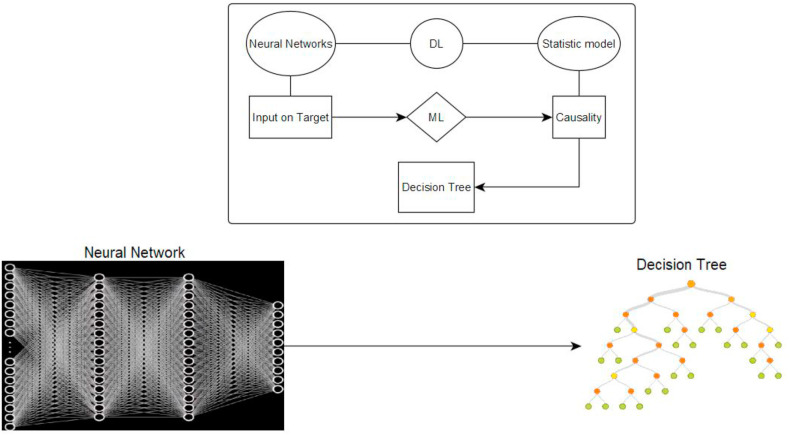
Following Magazzino et al. (2020c) and Mele and Magazzino (2020b), we demonstrate how high levels of air pollutants lead to a higher probability, both direct and indirect, of an exponential increase in the number of COVID-19 deaths. To do so, we use the approach presented in Magazzino et al. (2020c) and a Deep Learning method applied to ANNs tested with the Tree Model in ML (Magazzino et al., 2020a, 2020b, 2020c, 2020d, 2021; 2020b; Mele and Magazzino, 2020a, 2020b). ANNs architectures built on this dataset are selected via Incremental Order Test that endures a huge number of combinations of neural signals, both inputs, and outputs, through logistic and hyperbolic activation functions. Once built, the neural structure is tested via Training Strategy (Training-Selection and Testing test), with the expected outcome derived using Plot Direction Output. The outcome is a “critical” threshold level of fine particulate concentration (in μg/m3) in the atmosphere for New York state, compared to the number of COVID-19 deaths. We perform our analysis in DML following the process shown in Fig. 1 .
Fig. 1.
DML process.
Source: our elaborations in Yed Graph Editor.
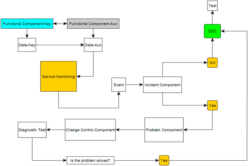
Once the dataset is built, the NN architecture is chosen and we process a Deep Learning approach in the Oryx protocol. We carry out statistical tests on the series of data used. These tests express the correct preparation of the dataset. Subsequently, we identify the inputs and target of the first model concerning a hyperbolic or logistic activation function. Then, we identify through tests in ML, the correctness of the chosen architecture, and if not right, we build n NN. We then select the NN that has a minor prediction error. Subsequently, we verify the link of causality through the “shear” procedure using a decision tree model through the BIGL package in ML. According to Hu et al. (2012), the second experiment is a D2C (ML) causality model. We use the result of the hyperbolic equations of the first experiment by adding the change in the economic growth of the state of New York. For the variable representing economic growth (rGDP), we use the change in real GDP.2 We perform our analysis in D2C-ML following the process shown in Fig. 2 .
Fig. 2.
D2C ML process.
Source: our elaboration in Yed Graph Editor.
The D2C auxiliary analysis is complex with two interconnected starting points: Functional Component Key and Functional Component Aux. The first derives from the dataset used for the NN in which the variable relating to real Gross Domestic Product (GDP) has been added. The second, on the other hand, represents a set of hyperbolic equations that are a result of the NN process. These two datasets make up the Service Monitoring that generates the event to be analyzed. Subsequently, an Incident Component is generated without supervision necessary to verify the correctness of the distribution of the two datasets. If this test fails, we produce the D2C causality model. If not, we analyze the presence of control errors in the system through diagnostic tests.
4. Empirical results
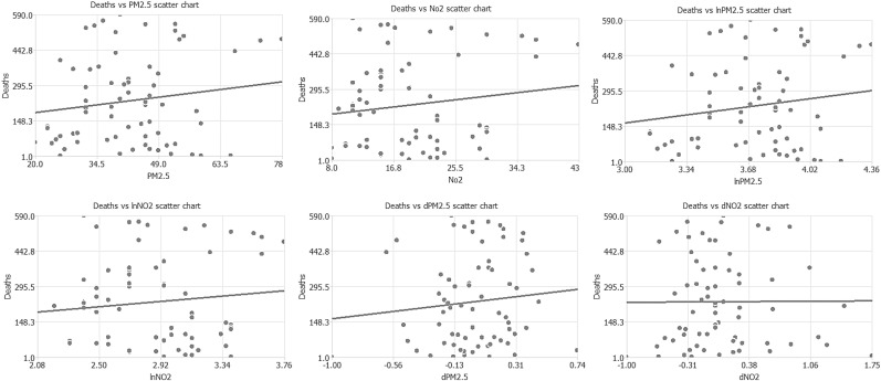
Generally, before analyzing the results of an empirical time series methodology, it is necessary to examine the time series properties of the variables and the presence of cointegration. However, according to Sundararajan et al. (2017), an experiment in DML considers a dataset as a stationary element. Hence, analysis is not affected by the presence of a time series in the data. Therefore, once the dataset was created in CSV and forwarded within the NN protocol, we observed the distribution of the data. Table A in Appendix represents the summary of the dataset used in the Oryx processing of the NN. The variables used are 9, of which 8 represent the input process, and 1 is the generated target. Fig. 3 shows the plot scatter chart of all variables, whilst we report the behaviour of the instances through a pie chart elaborated by the protocol in Figure A in Appendix.
Fig. 3.
Plot scatter chart.
Source: our elaborations Oryx 2 - Apache Spark.
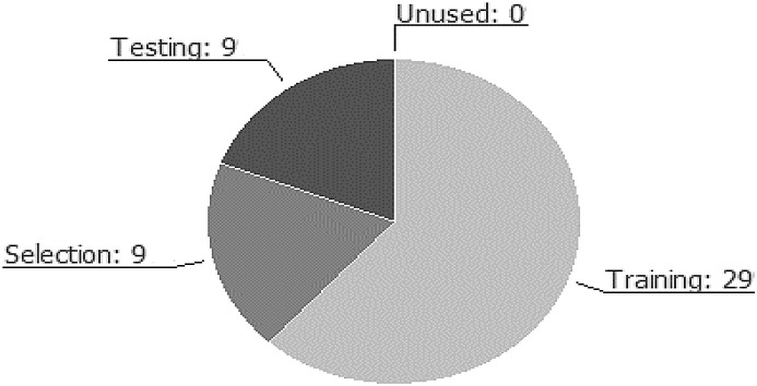
The instances generated by the automatic intelligence process are 47. Of these, training is the most important since it has 29 instances (61.7%). This first result highlights how, on an automatic level, the process could select 29 models capable of best estimating the target out of a total of 47 potential ML projects. As for the requests relating to the selection, they are equal to 9, which is 19% of the total requests. This value for the theory of NN must be lower than that of the training instances. Therefore, this result also confirms the goodness of the model generated through the NN. The result of the “instant selection” provides another interpretation if compared with the instances testing. Their value is the same (testing 9) and therefore, the models selected by the previous instances are all potentially testable in the NN. Finally, we can see that there are no unused instances (unused = 0) and therefore, no outliers were generated that would invalidate the results. The results obtained from the instances’ analysis confirm the possibility of generating a NN according to the architecture chosen by the operator.
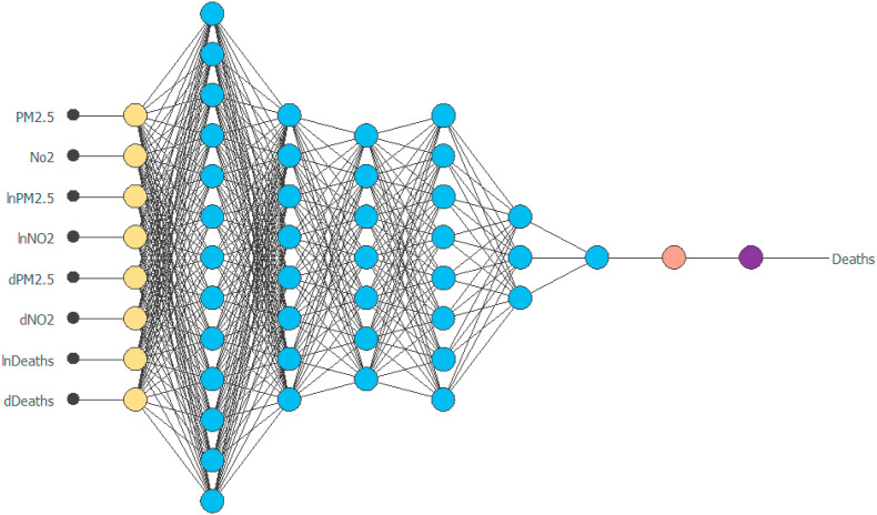
The result of the graphic elaboration of the NN with 8 inputs and 1 output generated in Oryx with Designer extension version 1.8 is depicted in Figure B in Appendix. The architecture of the NN reveals a complexity, represented by hidden neurons, of 13:8:7:11:3. The distribution of the NN is not of the linear type but has 2 redundant neural states that are active towards the end of the NN. While the yellow filled circles represent the scaling neurons, the blue filled circles are the perceptron neurons, whereas the red filled circles represent the unscaling neurons. The activation function chosen for this analysis is logistic, while a linear function generates the target. Each combination of the inputs generates the variation of COVID-19 deaths in a process with no anomalous values. Therefore, the plot of NN can be read as the n combinations of inputs that generate a variation of the target through a logistic combination with a linear result.
Once the NN is built, we proceed through numerous tests to validate the model. These tests assist the operator to identify the probability that there is a better algorithm different from the one chosen in the initial phase.
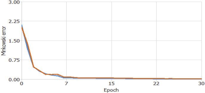
The analysis that tests our algorithm's goodness for the creation of the NN begins with the Perform Training using the Quasi-Newton method (Figure C in Appendix). It uses Newton's system of ANNs in ML process. However, compared to self-generated networks in which a “block of losses” is not selected, our test does not require secondary derivatives calculation. It is called “Quasi-Newton” because it calculates an approximation of the Hessian inverse to each recurring signal of the algorithm. In other words, it uses only the gradient information. Also, despite using standard deviation, we use the Minkowski error as a test with a minor index. The Minkowski error represents the failure test in ML with the highest performance and most significant fit in an ANN.
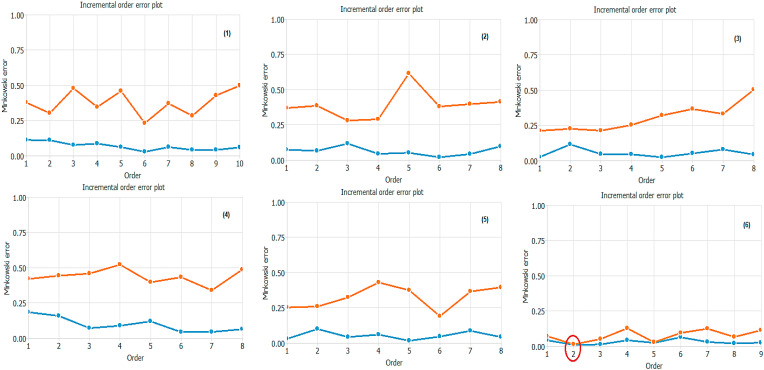
Figure C shows the training and selection errors in each iteration. The blue line shows the graph's training error, while the orange line represents the selection error. As we can see from the error trend, the training error shows a decreasing trend. It records a value of 1.9816 in its initial phase. However, after 12 epochs, the error drops to a value of 0.0383. As regards the trend of the selection error, it too has a decreasing trend. The value of 1.991 in its initial phase reaches a value of 0.0425 after 10 epochs. The decreasing trend of the two error tests concerning the increasing epochs highlights how our strategy has proved ideal for the NN elaboration process. The analysis that verifies the perfect performance of the NN also requires the Performed Order Selection test. This test suggests to the operator the model's choice, whose complexity is the most appropriate to produce an adequate data fit. This testing process is fully automatic and left to the interpretation of artificial intelligence guided by our algorithm. It is responsible for finding the optimal number of neurons in the network. This process takes place by combining our initial algorithm with the one pre-set by the software, the incremental order algorithm. Fig. 4 shows the error history for the different subsets during the incremental order selection process. The blue line shows the training error while the orange line symbolizes the selection error.
Fig. 4.
Incremental Order Error plot test. Notes: (1) 13:8:7: 11:6 MSE 0.21; (2) 13:8:7:11:3 MSE 0.35; (3) 13:8:7:11:2 MSE 0.25; (4) 13:8:7:11:7 MSE 0.30; (5) 13:8:7:9:6 MSE 0.22; (6) 13:8:7:8:3 MSE 0.03.
Source: our elaborations Oryx 2 – Apache Spark.
Both the training error and selection error decrease with increasing order in point number 2. These results highlight the presence of a better-hidden architecture. It presents even lower algorithm errors than our initial architecture. Therefore, following the ML process in Fig. 5 , we elaborate on the final architecture of this NN.
Fig. 5.
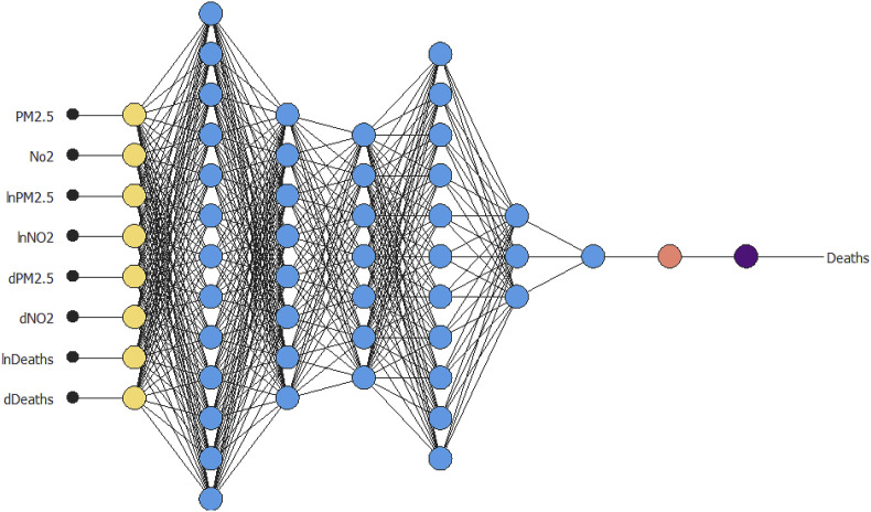
Final architecture ANNs results.
Source: our elaborations Oryx 2 – Apache Spark.
The results of our elaboration in light of the findings achieved with the Perform Order Selection test are presented in Fig. 5. Based on 8 inputs and 1 output variable, the complexity is 10:8:2, represented by the numbers of hidden neurons. Therefore, compared to Figure B, this NN presents an automatic choice that has reduced the fourth hidden layer of the neuron. The target generated by the NN process remains the same and identifiable in the variation of per capita GDP.
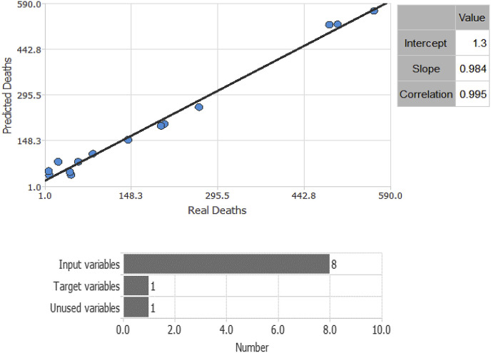
Subsequently, to ensure the most appropriate goodness of the results in a model of black networks, we test the final architecture through several operations. One of these is to perform a linear regression analysis between the scaled NN outputs and corresponding targets for an independent test subset (Figure D in Appendix). This important analysis in a predictive model considers three parameters for each output variable. The first two parameters, referable to letters a and b, correspond to the y-intercept and slope of the best predictive linear regression related to the targets which are scaled. The third parameter is the usual R-square, already widely used in statistics and econometrics.
The prediction line (with respect to the target, Deaths) perfectly confirms the goodness of the elaborated algorithm on the final architecture. The prediction shows an intercept of 1.3, very high correlation value (0.995), and slope of 0.984, implying a slope close to unity. Now, we examine the input that influences the target's prediction (to a greater extent) to ascertain the process of economic growth. To this end, we enrich our algorithm with the “Model deployment” protocol developed by Artificial Intelligence Techniques, Ltd. This protocol generates the weight of all the inputs in NN, concerning the target.
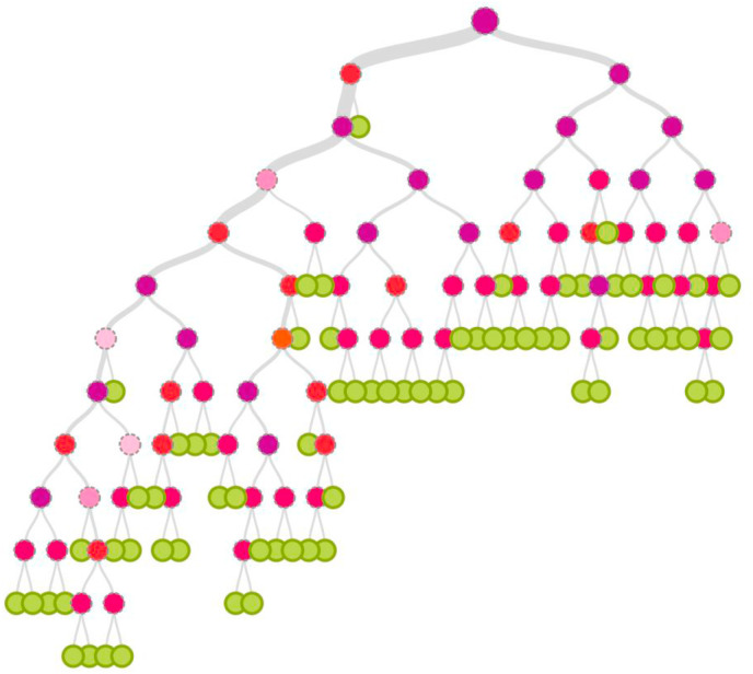
The results of the 8 inputs used for our final architecture of the NN are presented in Table B in Appendix. All variables (and their transformations) have positive values. Of all the inputs, we can observe that the most significant positive value is represented by PM2.5 and NO2. These results confirm that air pollution plays an essential role in facilitating COVID-19 attributable deaths. The transform versions of the variables have lower values, hence, we test these results through the so-called “Decision Tree Model” (Fig. 6 ). Our decision tree is a system with n input and output variables. Input variables (attributes) are derived from observation of the environment. The last output variables, on the other hand, identify the decision/action to be taken. Decision making is represented by an inverted logical tree where each node is a conditional function. Each node tests a condition (test) on a particular property of the environment (variable) and has two or more downward branches in operation. The process consists of a sequence of tests. It always starts from the root node, parent node located higher in the structure, and proceeds downwards. Depending on the values detected in each node, the flow takes one direction or another and proceeds progressively downwards. The final decision is found in the terminal leaf nodes, the lower ones. In this way, after analyzing the various conditions, the agent reaches the final decision.
Fig. 6.
Decision tree model.
Source: our elaborations in BML – IBM.
The target value on our decision tree in Fig. 6 is COVID-19 deaths whereas the initial question is how PM2.5 and NO2 interplay in causation. In the left part of the tree, the answer is yes while on the right side, the answer is no. We note that the left part of the tree immediately shows a final reply attributable to a green dot compared to a purple one. Since the green dot is the probability that air pollutant emissions cause COVID-19 deaths, we instantly register an affirmative response of 50%. The decision tree confirms that compared to an alternative choice, pollutant emissions exacerbate deaths from COVID-19 in New York state.
We further perform Deep Learning approach with D2C (ML) causality tests to determine the relationship between the sampled variables. We use the results of the hyperbolic equations of the first experiment in ANNs by adding the change in the economic growth of the state of New York (rGDP). In the model, n filtered factors are used (which do not appear in Table 1 ) to perform the task of training the classification of our model. Thirty-six classifiers are trained and tested by the self-learning machine to achieve the predictive causal link between the variables. These thirty-six classifiers work through a binary calculation sequence, alternating the values [0] and [1].
Table 1.
The rank of predictor and significant causality results for New York (D2C).
| Rank of Predictor | Number of repetitions | Percentage (%) | AC | AUPRC |
|---|---|---|---|---|
| PM2.5→NO2 | 17985 | 0.89 | 4.949 | False |
| PM2.5←NO2 | 17549 | 0.88 | 4.784 | False |
| lnPM2.5→lnNO2 | 18161 | 0.94 | 4.745 | False |
| lnPM2.← lnNO2 | 18542 | 0.93 | 4.197 | False |
| dPM2.5→dNO2 | 18965 | 0.77 | 4.106 | False |
| dPM2.←dNO2 | 18954 | 0.75 | 4.174 | False |
| PM2.5→Deaths | 21756 | 0.72 | 4.100 | True |
| PM2.5←Deaths | 21479 | 0.73 | 4.105 | False |
| lnPM2.5→lnDeaths | 17456 | 0.89 | 4.922 | False |
| lnPM2.5←lnDeaths | 17479 | 0.87 | 4.723 | False |
| dPM2.5→dDeaths | 18165 | 0.93 | 4.711 | False |
| dPM2.5←dDeaths | 18195 | 0.92 | 4.195 | False |
| NO2→Deaths | 18985 | 0.75 | 4.101 | True |
| NO2←Deaths | 18962 | 0.74 | 4.174 | False |
| lnNO2→lnDeaths | 21962 | 0.72 | 4.104 | True |
| lnNO2←lnDeaths | 21008 | 0.71 | 4.107 | False |
| dNO2→dDeaths | 17984 | 0.88 | 4.914 | False |
| dNO2←dDeaths | 17522 | 0.88 | 4.734 | False |
| rGDP→PM2.5 | 18165 | 0.92 | 4.744 | True |
| rGDP←PM2.5 | 18542 | 0.93 | 4.191 | False |
| ln.rGDP→lnPM2.5 | 18495 | 0.74 | 4.101 | False |
| ln.rGDP←lnPM2.5 | 18184 | 0.76 | 4.171 | False |
| d.rGDP→dPM2.5 | 21654 | 0.77 | 4.102 | True |
| d.rGDP←dPM2. | 21966 | 0.78 | 4.102 | False |
| rGDP→NO2 | 17445 | 0.81 | 4.941 | False |
| rGDP←NO2 | 17951 | 0.82 | 4.783 | False |
| ln.rGDP→lnNO2 | 18495 | 0.92 | 4.749 | False |
| ln.rGDP←lnNO2 | 18795 | 0.95 | 4.197 | False |
| d.rGDP→dNO2 | 18116 | 0.74 | 4.104 | True |
| d.rGDP←dNO2 | 18496 | 0.77 | 4.175 | False |
| rGDP→Deaths | 21984 | 0.75 | 4.106 | False |
| rGDP←Deaths | 21956 | 0.74 | 4.102 | False |
| ln.rGDP→lnDeaths | 18494 | 0.71 | 4.107 | False |
| ln.rGDP←lnDeaths | 18961 | 0.71 | 4.171 | False |
| d.rGDP→dDeaths | 21445 | 0.72 | 4.109 | False |
| d.rGDP←dDeaths | 21411 | 0.72 | 4.108 | False |
Notes: AC: Average Causality value. AUPRC: Area Under the Precision-Recall Curve. True: P-Value < 0.05. False: P-Value ≥ 0.05.
Source: our elaborations Oryx 2 – Apache Spark.
Table 1 clearly shows how our algorithm performed numerous repetitions for each combination of causality between the variables. On average, these combinations recorded a value of 19,500 repetitions. The item “Percentage (%)” represents the closing percentages of the calculation within the 19,500 repetitions average. The results of this item of the predictive causation process have always been greater than 70%. This highlights how our algorithm can complete each cycle for each pair of variables. The mean causality value is uniform for all pairs of values analyzed. The item “AUPRC” represents the one able to report the level of significance of the results of predictive causality. Compared to normal prediction models, it uses the binary system (0 or 1) to formulate the question “true or false” regarding the P-Value lower or higher than 5%. We observe only six significant causal relationships within the AUPRC analysis. The causal relationships are attributable to a one-way causality ranging from PM 2.5 to Deaths, NO 2 to Deaths, from lnNO 2 to lnDeaths, from rGDP to PM 2.5, from d.rGDP to dPM 2.5 , and from d.rGDP to dNO 2. These results confirm that the “polluting” variables have a predictive causality that stimulates the death of COVID-19. The result obtained is different from those obtainable from alternative models to our algorithm. The previously identified causal links represent the result of our ML model's autonomous action. In other words, it has combined numerous processes without the intervention of an external operator – but only by analyzing the environment of the variables that make up the dataset. Indeed, adding GDP, the experiment shows that economic growth declines environmental sustainability by promoting high emissions of fine particulate matter and carbon dioxide.
5. ML test on control cities
To test the results obtained on the state of New York, we selected two cities: Tokyo and Milan. We chose these two control cities because they show different epidemiological and environmental patterns from official statistical sources between March and December 2020. These cities are characterized by dynamic economies: Milan has a GDP of 367 billion dollars compared to Tokyo (excluding greater Tokyo area) with a GDP of 1857 billion dollars in 2019. Although these two cities represent financial centers with a medium-high population density but recorded a different contagion/death ratio from Covid-19 during the pandemic. Milan recorded contagion/death value of 5.12%, whereas Tokyo recorded about 1% contagion/death value. This result may be attributable to numerous determinants including health system efficiency, virus containment, and environmental measures. Since Tokyo implemented a strict infection tracking policy, the city recorded low levels of PM2.5 and NO2.
On the other hand, Milan failed in the tracking policy, recording high levels of PM2.5 and NO2. We, therefore, applied the D2C predictive causation model to the two cities. In other words, we adopted the same ML model used for the state of New York to verify whether the number of deaths-related to Covid-19 in the two cities was influenced (predictively and without supervision) by the levels of environmental pollution. Since Tokyo implemented a social control policy by tracing the infected population, we inserted a controlling factor––the so-called “matrix approximate control”. In this way, the algorithm was able to equate only the two cities regarding environmental effects.
The results obtained from the predictive causality system in ML confirm previous findings for New York. If we observe the model's results for Tokyo (Table 2, Table 4 ), we find no relationship between Covid-19 deaths and emissions (AUPRC). Almost all of the choices between true and false events have fallen on false events. Moreover, the model presented an identified AC value for all combinations on predictive causality. This result, undoubtedly influenced by the control matrix reveals no discrepant value capable of hypothesizing an event error between true and false events. The results, however, were entirely different from the city of Milan (Table 3, Table 5 ). It recorded poorly than that of New York State on the link between pollutants and deaths from Covid-19. In our model, the predictive causality was recorded for each variable transformed (ln. or d.). In other words, the unsupervised algorithm interprets such events in all forms of variation: stable, logarithmic, or in first difference, consistent with Magazzino et al. (2020b).
Table 2.
The rank of predictor and significant causality results for Tokyo (D2C).
| Rank of Predictor | Number of repetitions | Percentage (%) | AC | AUPRC |
|---|---|---|---|---|
| PM2.5→NO2 | 21478 | 0.89 | 4.850 | False |
| PM2.5←NO2 | 21595 | 0.89 | 4.850 | False |
| lnPM2.5→lnNO2 | 20891 | 0.90 | 4.850 | False |
| lnPM2.←lnNO2 | 19529 | 0.91 | 4.850 | False |
| dPM2.5→dNO2 | 19855 | 0.89 | 4.850 | False |
| dPM2.←dNO2 | 20195 | 0.89 | 4.850 | False |
| PM2.5→Deaths | 19592 | 0.89 | 4.950 | False |
| PM2.5←Deaths | 20945 | 0.80 | 4.850 | False |
| lnPM2.5→lnDeaths | 19795 | 0.80 | 4.850 | False |
| lnPM2.5←lnDeaths | 19785 | 0.80 | 4.850 | False |
| dPM2.5→dDeaths | 19829 | 0.90 | 4.850 | False |
| dPM2.5←dDeaths | 18195 | 0.90 | 4.850 | False |
| NO2→Deaths | 18555 | 0.80 | 4.850 | False |
| NO2←Deaths | 18772 | 0.80 | 4.850 | False |
| lnNO2→lnDeaths | 20268 | 0.90 | 4.850 | False |
| lnNO2←lnDeaths | 21952 | 0.80 | 4.850 | False |
| dNO2→dDeaths | 19532 | 0.80 | 4.850 | False |
| dNO2←dDeaths | 19523 | 0.80 | 4.850 | False |
| rGDP→PM2.5 | 19255 | 0.80 | 4.850 | False |
| rGDP←PM2.5 | 19663 | 0.85 | 4.950 | False |
| ln.rGDP→lnPM2.5 | 18522 | 0.85 | 4.850 | False |
| ln.rGDP←lnPM2.5 | 18122 | 0.85 | 4.850 | False |
| d.rGDP→dPM2.5 | 20955 | 0.80 | 4.850 | True |
| d.rGDP←dPM2. | 28289 | 0.80 | 4.850 | False |
| rGDP→NO2 | 19523 | 0.80 | 4.850 | False |
| rGDP←NO2 | 19552 | 0.80 | 4.850 | False |
| ln.rGDP→lnNO2 | 18112 | 0.90 | 4.850 | False |
| ln.rGDP←lnNO2 | 18899 | 0.90 | 4.850 | False |
| d.rGDP→dNO2 | 19525 | 0.80 | 4.850 | True |
| d.rGDP←dNO2 | 19654 | 0.80 | 4.850 | False |
| rGDP→Deaths | 20258 | 0.85 | 4.850 | False |
| rGDP←Deaths | 20269 | 0.85 | 4.850 | False |
| ln.rGDP→lnDeaths | 19745 | 0.80 | 4.850 | False |
| ln.rGDP←lnDeaths | 19226 | 0.75 | 4.850 | False |
| d.rGDP→dDeaths | 20236 | 0.70 | 4.850 | False |
| d.rGDP←dDeaths | 22596 | 0.80 | 4.850 | False |
Notes: AC: Average Causality value. AUPRC: Area Under the Precision-Recall Curve. True: P-Value < 0.05. False: P-Value ≥ 0.05.
Source: our elaborations with Oryx 2 – Apache Spark.
Table 4.
Optimization Test in Machine Learning results for Tokyo.
| Value | |
|---|---|
| Final parameters norm | 701 |
| Final training error | 0.044 |
| Final selection error | 0.0916 |
| Final gradient norm | 0.0132 |
| Epochs number | 597 |
| Elapsed time | 00:00 |
| Stopping criterion | Maximum selection error increases |
Source: our elaborations with Oryx 2 – Apache Spark.
Table 3.
The rank of predictor and significant causality results for Milan (D2C).
| Rank of Predictor | Number of repetitions | Percentage (%) | AC | AUPRC |
|---|---|---|---|---|
| PM2.5→NO2 | 17752 | 0.80 | 4.945 | False |
| PM2.5←NO2 | 17965 | 0.88 | 4.785 | False |
| lnPM2.5→lnNO2 | 18711 | 0.95 | 4.745 | False |
| lnPM2.←lnNO2 | 18785 | 0.91 | 4.195 | False |
| dPM2.5→dNO2 | 18195 | 0.75 | 4.105 | False |
| dPM2.←dNO2 | 18785 | 0.75 | 4.175 | False |
| PM2.5→Deaths | 21015 | 0.75 | 4.105 | True |
| PM2.5←Deaths | 21252 | 0.75 | 4.100 | False |
| lnPM2.5→lnDeaths | 17896 | 0.88 | 4.905 | True |
| lnPM2.5←lnDeaths | 17785 | 0.88 | 4.705 | False |
| dPM2.5→dDeaths | 18785 | 0.90 | 4.705 | True |
| dPM2.5←dDeaths | 18785 | 0.90 | 4.190 | False |
| NO2→Deaths | 18777 | 0.75 | 4.105 | True |
| NO2←Deaths | 18785 | 0.75 | 4.175 | False |
| lnNO2→lnDeaths | 21788 | 0.75 | 4.105 | True |
| lnNO2←lnDeaths | 21785 | 0.75 | 4.105 | False |
| dNO2→dDeaths | 17855 | 0.85 | 4.900 | True |
| dNO2←dDeaths | 17555 | 0.85 | 4.700 | False |
| rGDP→PM2.5 | 18178 | 0.90 | 4.905 | True |
| rGDP←PM2.5 | 18581 | 0.90 | 4.105 | False |
| ln.rGDP→lnPM2.5 | 18488 | 0.75 | 4.105 | True |
| ln.rGDP←lnPM2.5 | 18188 | 0.75 | 4.175 | False |
| d.rGDP→dPM2.5 | 21852 | 0.75 | 4.105 | True |
| d.rGDP←dPM2. | 21881 | 0.75 | 4.105 | False |
| rGDP→NO2 | 17785 | 0.80 | 4.905 | True |
| rGDP←NO2 | 17852 | 0.85 | 4.705 | False |
| ln.rGDP→lnNO2 | 18852 | 0.90 | 4.705 | True |
| ln.rGDP←lnNO2 | 18726 | 0.90 | 4.105 | False |
| d.rGDP→dNO2 | 18155 | 0.75 | 4.105 | True |
| d.rGDP←dNO2 | 18785 | 0.75 | 4.175 | False |
| rGDP→Deaths | 21523 | 0.75 | 4.105 | False |
| rGDP←Deaths | 21781 | 0.75 | 4.105 | False |
| ln.rGDP→lnDeaths | 18852 | 0.75 | 4.105 | False |
| ln.rGDP←lnDeaths | 18299 | 0.75 | 4.175 | False |
| d.rGDP→dDeaths | 21881 | 0.75 | 4.105 | False |
| d.rGDP←dDeaths | 21855 | 0.75 | 4.105 | False |
Notes: AC: Average Causality value. AUPRC: Area Under the Precision-Recall Curve. True: P-Value < 0.05. False: P-Value ≥ 0.05.
Source: our elaborations with Oryx 2 – Apache Spark.
Table 5.
Optimization Test in Machine Learning results for Milan.
| Value | |
|---|---|
| Final parameters norm | 6.72 |
| Final training error | 0.0445 |
| Final selection error | 0.0962 |
| Final gradient norm | 0.0356 |
| Epochs number | 612 |
| Elapsed time | 00:00 |
| Stopping criterion | Maximum selection error increases |
Source: our elaborations with Oryx 2 – Apache Spark.
Finally, Table 4, Table 5 show the goodness of our results. Regarding Tokyo, the algorithm analyzed a predictive path of 597 epochs. After 7.01 epochs, training and selection error recorded its lowest value. The orthogonal matrices preserve gradient norm during backpropagation to a value of 0.0132, confirming the model's optimality. On the other hand, the test on Milan required several major epochs (612). However, the control parameters were normalized to a lower epoch level (6.72). The training and selection error results are low and within a range of 1–10%. The final gradient norm is in line with DML theory and lower than the two previous tests.
6. Concluding remarks and policy recommendations
This study estimated the relationship between air quality and high levels of COVID-19 attributed deaths in New York state, USA. In a bid to have a clear path of unveiling this study, we considered the interaction of pollution, economic growth, and COVID-19 deaths as better indexes and proxies in measuring environmental and economic impacts. Our empirical results confirmed the nexus among unsustainable growth, air pollution, and the spread of COVID-19 pandemic in New York state. We employed two experimental approaches based on DML experience for a thorough investigation of the proposed theme. The first experiment assessed the relationship between pollution and the number of deaths from COVID-19, while the second experiment performed the hyperbolic equations of the first expression in generating the causal inferences among the chosen variables. The findings based on the two experiences are as follows: First, PM2.5 and NO2 are confirmed to be the most significant pollutant agents responsible for facilitating death rates caused by COVID-19. The decision tree affirmed with a 50% response rate that deaths from COVID-19 in New York are possibly caused by air pollutants. From the second experiment, we found only six significant and true within the AUPRC analysis to test causal inferences. In line with the causal findings, a unidirectional causal effect was found in the analysis — extending from PM 2.5 to Deaths, NO 2 to Deaths, lnNO 2 to lnDeaths, rGDP to PM 2.5, d.rGDP to dPM 2.5, and d.rGDP to dNO 2. Similarly, to the first experiment, the causal result confirmed the escalation effect of polluting variables (PM 2.5 to Deaths, NO 2 to Deaths) on COVID-19 deaths. Importantly, increasing levels of economic growth (rGDP to PM 2.5, d.rGDP to dPM 2.5, and d.rGDP to dNO 2) spur air pollutants, hence, act as a catalyst for increasing ambient air pollution. This implies a pollution-embedded economic growth in New York state that thwarts environmental sustainability by eventually activating emissions of pollutant agents (PM2.5 and NO2). The resulting effect of emissions from pollutant agents is the spread of viruses such as COVID-19—which could trigger more deaths in New York.
The empirical evidence showed the impact of COVID-19 pandemic in New York is majorly caused by the fast spread of pollutant agents due to emission-embedded economic growth. Thus, the following policy recommendations emanate from the study: To build a lasting solution in containing the impact of COVID-19 pandemic and future occurrences, Government intervention policies could encourage decarbonization of economic development through pollution abatement technologies. A call for a paradigm shift is inevitable through the adoption of research, development, and innovations across economic sectors. Decoupling economic growth from air pollution requires the dependence on renewable and low carbon energy to reduce emissions from the manufacturing sector. Awareness of a healthy and clean environment could be an effective tool in limiting the fast spread of the virus. The heterogeneous nature of countries across the globe and complexity of COVID-19 appears a limiting factor of our study to achieve homogeneous results, however, our empirical procedure set a foundation for future research necessary to curtail the effect of COVID-19 and future pandemics.
Finally, a decrease in air pollutants might decrease the global temperature through a decline in GHG emissions that may in-turn increase the infectivity – and possibly mortality – of COVID-19 (Haque and Rahman, 2020). Therefore, future research may possibly investigate the role of other pollutant species on the stability and spread of the global pandemic while controlling for other confounders.
Credit author statement
Cosimo Magazzino: Conceptualization, Methodology, Software, Supervision. Marco Mele: Visualization, Investigation, Validation, Writing-Reviewing and Editing. Samuel Asumadu Sarkodie: Writing – original draft , Writing-Reviewing and Editing.
Declaration of competing interest
The authors declare that they have no known competing financial interests or personal relationships that could have appeared to influence the work reported in this paper.
Acknowledgments
Open Access funding provided by Nord University.
Footnotes
Nomenclature
- ANNs
Artificial Neural Networks
- CIS
Commonwealth of Independent States
- CO2
Carbon Dioxide
- COVID-19
Coronavirus Disease 19
- D2C
Causal Direction from Dependency
- DML
Deep Machine Learning
- GDP
Gross Domestic Product
- GHG
Greenhouse Gas
- GMM
Generalized Method of Moments
- ML
Machine Learning
- NN
Neural Network
- NO
Nitric Oxide
- NO2
Nitrogen Dioxide
- O3
Ozone
- PM2.5
Particulate Matter with an aerodynamic diameter <2.5 μm
- PM10
Particulate Matter with an aerodynamic diameter <10.0 μm
- VECM
Vector Error Correction Model
- WHO
World Health Organization
Appendix.
Fig. A.
Instances pie chart. Source: our elaborations Oryx 2 – Apache Spark.
Fig. B.
ANNs results.Source: our elaborations Oryx 2 – Apache Spark.
Fig. C.
Quasi-Newton method algorithm error history. Source: our elaborations Oryx 2 – Apache Spark.
Fig. D.
Predictive Linear Regression test. Source: our elaborations Oryx 2 – Apache Spark.
Table A.
Variables bars chart
Source: our elaborations in Oryx 2 – Apache Spark.
Table B.
Input on the target.
| Input name | Value |
|---|---|
| PM2.5 | 49 |
| NO2 | 25.500 |
| lnPM2.5 | 3.676 |
| lnNO2 | 2.920 |
| dPM2.5 | 0.130 |
| dNO2 | 0.375 |
| lnDeaths | 3.190 |
| dDeaths | 0.520 |
Source: our elaborations Oryx 2 – Apache Spark.
References
- Akbari H., Taghizadeh-Hesary F., Heike Y., Bahadori M. Cell energy: a new hypothesis in decoding cancer evolution. Arch. Iran. Med. 2019;22(12):733–735. [PubMed] [Google Scholar]
- Bengalli R., Zerboni A., Marchetti S., Longhin E., Priola M., Camatini M., Mantecca P. In vitro pulmonary and vascular effects induced by different diesel exhaust particles. Toxicol. Lett. 2019;306:13–24. doi: 10.1016/j.toxlet.2019.01.017. [DOI] [PubMed] [Google Scholar]
- Bildirici M.E. The causal link among militarization, economic growth, CO2 emission, and energy consumption. Environ. Sci. Pollut. Res. 2017;24(5):4625–4636. doi: 10.1007/s11356-016-8158-z. [DOI] [PubMed] [Google Scholar]
- Caliendo L., Parro F., Rossi-Hansberg E., Sarte P.D. The impact of regional and sectoral productivity changes on the U.S. economy. Rev. Econ. Stud. 2018;85(4):2042–2096. [Google Scholar]
- Cao C., Jiang W., Wang B., Fang J., Lang J., Tian G., Jiang J., Zhu T.F. Inhalable microorganisms in Beijing's PM2.5 and PM10 pollutants during a severe smog event. Environ. Sci. Technol. 2014;48:1499–1507. doi: 10.1021/es4048472. [DOI] [PMC free article] [PubMed] [Google Scholar]
- Chen R.J., Chen B.H., Kan H.D. A health-based economic assessment of particulate air pollution in 113 Chinese cities. China Environ. Sci. 2010:410–415. [Google Scholar]
- Ciencewicki J., Jaspers I. Air pollution and respiratory viral infection. Inhal. Toxicol. 2007;19(14):1135–1146. doi: 10.1080/08958370701665434. [DOI] [PubMed] [Google Scholar]
- Després V.R., Huffman J.A., Burrows S.M., Hoose C., Safatov A.S., Buryak G., Fröhlich-Nowoisky J., Elbert W., Andreae M.O., Pöschl U., Jaenicke R. Primary biological particles in the atmosphere: a review. Tellus B. 2012;64:15598. [Google Scholar]
- Dominici F., Wu X., Nethery R., Sabath B., Braun D. medRxiv; 2020. Exposure to Air Pollution and COVID-19 Mortality in the United States: A Nationwide Cross-Sectional Study. [DOI] [PMC free article] [PubMed] [Google Scholar]
- Donev D., Zaletel-Kragelj L., Bjegovic V., Burazeri G. Measuring the burden of disease: disability-adjusted life year (DALY) Methods and Tools in Public Health. 2010;30:715. [Google Scholar]
- Eckelman M.J., Sherman J. Environmental impacts of the U.S. health care system and the effects on public health. PloS One. 2016;11(6) doi: 10.1371/journal.pone.0157014. e0157014. [DOI] [PMC free article] [PubMed] [Google Scholar]
- Esquivel-Fariña A., Camelo-García V.M., Kitajima E.W., Rezende J.A.M., González-Segnana L.R. First report of wheat stripe mosaic virus in Paraguay. Australas. Plant Dis. Notes. 2019;14:24. [Google Scholar]
- Gupta M.R., Dutta P.B. Tourism development, environmental pollution, and economic growth: a theoretical analysis. J. Int. Trade Econ. Dev. 2018;27(2):125–144. [Google Scholar]
- Haque S.E., Rahman M. Association between temperature, humidity, and COVID-19 outbreaks in Bangladesh. Environ. Sci. Pol. 2020;114:253–255. doi: 10.1016/j.envsci.2020.08.012. [DOI] [PMC free article] [PubMed] [Google Scholar]
- Koondhar M.A., Qiu L., Li H., Liu W., He G. A nexus between air pollution, energy consumption, and growth of the economy: a comparative study between the USA and China-based on the ARDL bound testing approach. Agric. Econ. 2018;64(6):265–276. [Google Scholar]
- Lei L., Wu S., Lu S., Liu M., Song Y., Fu Z., He D. Microplastic particles cause intestinal damage and other adverse effects in zebrafish Danio rerio and nematode Caenorhabditis elegans. Sci. Total Environ. 2018;619–620:1–8. doi: 10.1016/j.scitotenv.2017.11.103. [DOI] [PubMed] [Google Scholar]
- Li Q., Guan X., Wu P., Wang X., Zhou L., Tong Y., Feng Z. Early transmission dynamics in Wuhan, China, of novel coronavirus-infected pneumonia. N. Engl. J. Med. 2020;382:1199–1207. doi: 10.1056/NEJMoa2001316. [DOI] [PMC free article] [PubMed] [Google Scholar]
- Liu Q., Lim S.H. Toxic air pollution and container port efficiency in the USA. Marit. Econ. Logist. 2017;19(1):94–105. [Google Scholar]
- Magazzino C., Mele M., Schneider N. A Machine Learning approach on the relationship among solar and wind energy production, coal consumption, GDP, and CO2 emissions. Renew. Energy. 2020;167:99–115. [Google Scholar]
- Magazzino C., Mele M., Schneider N. The relationship between air pollution and COVID-19-related deaths: an application to three French cities. Appl. Energy. 2020;279 doi: 10.1016/j.apenergy.2020.115835. [DOI] [PMC free article] [PubMed] [Google Scholar]
- Magazzino C., Mele M., Schneider N. The relationship between municipal solid waste and greenhouse gas emissions: evidence from Switzerland. Waste Manag. 2020;113:508–520. doi: 10.1016/j.wasman.2020.05.033. [DOI] [PubMed] [Google Scholar]
- Magazzino C., Mele M., Schneider N., Sarkodie S.A. Waste generation, Wealth and GHG emissions from the waste sector: is Denmark on the path towards Circular Economy? Sci. Total Environ. 2021;755(1):142510. doi: 10.1016/j.scitotenv.2020.142510. [DOI] [PMC free article] [PubMed] [Google Scholar]
- Magazzino C., Mele M., Schneider N., Vallet G. The relationship between nuclear energy consumption and economic growth: evidence from Switzerland. Environ. Res. Lett. 2020;15 [Google Scholar]
- Mele M., Magazzino C. A machine learning analysis of the relationship among iron and steel industries, air pollution, and economic growth in China. J. Clean. Prod. 2020;277 [Google Scholar]
- Mele M., Magazzino C. Pollution, economic growth and COVID-19 deaths in India. A machine learning evidence. Environ. Sci. Pollut. Res. 2020;28(3):2669–2677. doi: 10.1007/s11356-020-10689-0. [DOI] [PMC free article] [PubMed] [Google Scholar]
- Mahase E. Covid-19: what treatments are being investigated? Br. Med. J. 2020;368 doi: 10.1136/bmj.m1252. [DOI] [PubMed] [Google Scholar]
- Owusu P.A., Sarkodie S.A. Global estimation of mortality, disability-adjusted life years and welfare cost from exposure to ambient air pollution. Sci. Total Environ. 2020;742 doi: 10.1016/j.scitotenv.2020.140636. [DOI] [PubMed] [Google Scholar]
- Owusu PA, Sarkodie SA, Pedersen PA. Relationship between mortality and health care expenditure: Sustainable assessment of health care system. PLoS One. 2021;16(2) doi: 10.1371/journal.pone.0247413. [DOI] [PMC free article] [PubMed] [Google Scholar]
- Perrino C., Catrambone M., Dalla Torre S., Rantica E., Sargolini T., Canepari S. Seasonal variations in the chemical composition of particulate matter: a case study in the Po Valley. Part I: macro-components and mass closure. Environ. Sci. Pollut. Res. 2014;21:3999–4009. doi: 10.1007/s11356-013-2067-1. [DOI] [PubMed] [Google Scholar]
- Putrino A., Raso M., Magazzino C., Galluccio G. Coronavirus (COVID-19) in Italy: knowledge, management of patients and clinical experience of Italian dentists during the spread of contagion. BMC Oral Health. 2020;20:200. doi: 10.1186/s12903-020-01187-3. [DOI] [PMC free article] [PubMed] [Google Scholar]
- Remuzzi A., Remuzzi G. COVID-19 and Italy: What next? Lancet. 2020;395(10231):1225–1228. doi: 10.1016/S0140-6736(20)30627-9. [DOI] [PMC free article] [PubMed] [Google Scholar]
- Ritchie H., Roser M. Our World in Data; 2017. CO2and Greenhouse Gas Emissions. [Google Scholar]
- Rasoulinezhad E., Taghizadeh-Hesary F., Taghizadeh-Hesary F. How is mortality affected by fossil fuel consumption, CO2 emissions and economic factors in CIS region? Energies. 2020;13(9):2255. [Google Scholar]
- Sandberg M., Klockars K., Wilén K. Green growth or degrowth? Assessing the normative justifications for environmental sustainability and economic growth through critical social theory. J. Clean. Prod. 2019;206:133–141. [Google Scholar]
- Sarkodie S.A., Strezov V. An empirical study of the environmental Kuznets curve and environmental sustainability curve hypothesis for Australia, China, Ghana, and the USA. J. Clean. Prod. 2018;201:98–110. [Google Scholar]
- Sarkodie S.A., Owusu P.A. Impact of meteorological factors on COVID-19 pandemic: evidence from top 20 countries with confirmed cases. Environ. Res. 2020;191:110101. doi: 10.1016/j.envres.2020.110101. [DOI] [PMC free article] [PubMed] [Google Scholar]
- Sarkodie S.A., Owusu P.A. Global assessment of environment, health and economic impact of the novel coronavirus (COVID-19) Environ. Dev. Sustain. 2020:1–11. doi: 10.1007/s10668-020-00801-2. [DOI] [PMC free article] [PubMed] [Google Scholar]
- Sedlmaier N., Hoppenheidt K., Krist H., Lehmann S., Lang H., Büttner M. Generation of Avian Influenza Virus (AIV) contaminated fecal fine particulate matter (PM2.5): genome and infectivity detection and calculation of immission. Vet. Microbiol. 2009;139(1–2):156–164. doi: 10.1016/j.vetmic.2009.05.005. [DOI] [PubMed] [Google Scholar]
- Shapiro J.S., Walker R. Why is pollution from U.S. manufacturing declining? The roles of environmental regulation, productivity, and trade. Am. Econ. Rev. 2018;108(12):3814–3854. [Google Scholar]
- Sterpetti A.V. COVID-19 diffusion capability is its worst, unpredictable characteristic. How to visit a patient from a distance. Br. J. Surg. 2020;107(7):e181. doi: 10.1002/bjs.11644. [DOI] [PMC free article] [PubMed] [Google Scholar]
- Sundararajan M., Taly A., Yan Q. In: Proceedings of the 34th International Conference on Machine Learning. Precup D., The Y.W., editors. 2017. Axiomatic attribution for deep networks; pp. 3319–3328. [Google Scholar]
- Taghizadeh-Hesary F., Rasoulinezhad E., Yoshino N., Chang Y., Taghizadeh-Hesary F., Morgan P.J. The energy-pollution-health nexus: a panel data analysis of low- and middle-income Asian countries. Singapore Econ. Rev. 2020 doi: 10.1142/S0217590820430043. [DOI] [Google Scholar]
- Taghizadeh-Hesary F., Taghizadeh-Hesary F. The impacts of air pollution on health and economy in Southeast Asia. Energies. 2020;13(7):1812. [Google Scholar]


