Abstract
A wide range of dose reduction strategies for x-ray computed tomography (CT) have been investigated. Recently, denoising strategies based on machine learning have been widely applied, often with impressive results, and breaking free from traditional noise-resolution trade-offs. However, since typical machine learning strategies provide a single denoised image volume, there is no user-tunable control of a particular trade-off between noise reduction and image properties (biases) of the denoised image. This is in contrast to traditional filtering and model-based processing that permits tuning of parameters for a level of noise control appropriate for the specific diagnostic task. In this work, we propose a novel neural network that includes a spatial-resolution parameter as additional input permits explicit control of the noise-bias trade-off. Preliminary results show the ability to control image properties through such parameterization as well as the possibility to tune such parameters for increased detectability in task-based evaluation.
1. INTRODUCTION
X-ray CT has wide use in disease screening, diagnosis, and interventional guidance. Increasing CT use has raised concerns of excessive radiation dose to the population and encouraged the development of low-dose techniques. Due to the reduced number of photons in low-dose CT, reconstructed images contain higher noise making detection of small and low-contrast lesions more difficult. Algorithmic techniques including projection denoising, statistical iterative reconstruction, and image denoising have been developed for image quality improvement. Image denoising is applied to reconstructed images and can be easily integrated into existing CT pipelines. Image filters such as nonlocal means1 and block-matching 3D2 can reduce noise to a great extent. However, the filters generally do not attempt to directly model the noise distribution and may over-smooth the imaging resulting in loss of structural features. Recently, deep learning techniques have become very popular in image processing including denoising applications. Chen et al. designed a residual encoder-decoder convolutional network (RED-CNN) that suppresses noise and attempts to maintain structural features.3
Machine learning approaches differ from traditional processing in many ways. The ability of networks to learn distributions of both the noise properties and the underlying prior distribution of image content has distinct advantages over other approaches. Such methods are often able to provide results that are dramatic improvements over traditional noise-resolution trade-offs in classic methods. However, machine learning methods also differ in that they tend to provide only a single level of performance. That is, there generally is no provision for parametric control of how aggressive the noise reduction should be. While a single image output is convenient, this restricts radiologist preference and the ability to tune the level of noise reduction to the particular diagnostic task. For example, recent work has employed task-based metrics to optimize classic reconstruction methods as well as imaging system design for specific tasks.4
Image properties in machine learning approaches can be complex,5 and difficult to describe in terms of a classic noise-resolution trade-off. However, there is a more general noise-bias trade-off that is being made based on the particular loss function used to train the network. Biases can manifest as blur but also as other misrepresentations of the image volume including the elimination of specific structures or textures, and the injection of false features.
In this work, we propose a novel convolutional neural network (CNN) for low-dose CT denoising with a hyper-parameter σ that can be used to control the trade-off between noise reduction and bias. We consider a specific example where this σ induces different spatial resolutions in the denoised image (though other more general parameterizations of bias are possible). The proposed sigma-CNN (sCNN) provides a flexible selection of spatial resolution, allowing a user-defined balance between noise and bias for specific tasks.
2. METHODS
2.1. Generalized formulation for noise reduction with parametric control
In this work, we adopt a conventional monoenergetic CT model where the measurements are distributed y ~ Poisson(I0 exp{−Aμ}). where is the ground truth image volume. is the projection matrix, and I0 denotes the nominal fluence level. In low-dose CT. relatively low I0 increases the relative signal-to-noise ratio. Here, we focus on CT measurements that are reconstructed into an image estimate using filter-back projection (FBP). In conventional denoising. the trade-off between noise and resolution is often controlled with a single parameter. For example, a simple low-pass filter with a controllable cut-off frequency can effectively remove the high-frequency noise but with a sacrifice in spatial resolution. We seek to provide a generalized denoising method that has similar control of image properties such that
| (1) |
where is the denoised image with hyper-parameter σ that represents a particular level of bias in the restored image. Various bias metrics might be applied; however, we consider the familiar ease where σ represents a measure of spatial resolution. Thus, the general denoising problem is then summarized as finding the f(·) that can efficiently decrease the noise while controlling the overall blur by minimizing the following loss function,
| (2) |
where μ is the ground truth image (or, alternately a normal dose, low noise CT scan), and G(σ) is a Gaussian kernel with standard deviation σ. The loss function evaluates the mean squared error (MSE) between the estimated denoised image and the parameterized, blurred ground truth.
2.2. Neural network denoising with controllable spatial resolution
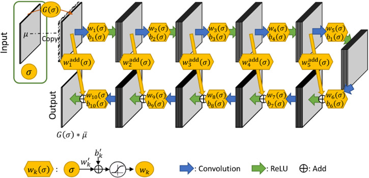
Many studies have investigated learning-based noise reduction in low-dose CT images, including the residual encoder-decoder convolutional neural network (RED-CNN)3 and the KAIST-Net.6 In this work, we adopt the overall architecture of the RED-CNN and add a second input for spatial resolution tuning (Figure 1).
Figure 1:
Architecture of the denoising CNN with spatial resolution control, where the resolution control components are color-coded with orange. The network receives two inputs: 1) the low-dose CT image and 2) a hyper-parameter σ for resolution control. The output is a denoised image at desired spatial resolution.
The RED-CNN incorporates serial 2D convolutional and deconvolutional layers as symmetric encoder and decoder components. Each convolutional/deconvolutional layer is followed by a rectified linear units (ReLU) activation layer:
| (3) |
where mk denotes the convolutional kernels and ak denotes the ReLU offsets in the kth convolutional layer. The notations μk+1, represent the output and input of the kth layer, respectively. The The stride of both convolution and deconvolutional layers are fixed to 1 to avoid down-sampling/up-sampling, and the size of each image/feature map in the output is consistent with the original image size. As a result, the implementations of the convolution and deconvolutional layers are essentially the same, and are denoted with convolution operator *. The filter number of all convolutional layers is a constant C, except for the last which is 1.
In the proposed network, the desired spatial resolution level σ is also an input to the network in addition to the low-dose CT image. Similarly, an additional blurred noisy image is generated with Gaussian filter and stacked with the original image as input to the convolutional layers. To interact with the convolutional layer, the single scalar is expanded through a fully-connected layer with sigmoid activation (Sigmoid(u) = (1 + e−u)−1) to generate a series of weights and biases wk(σ), bk(σ) that linearly transform the output of the convolutional layer:
| (4) |
| (5) |
where are channel-wise weights and offsets. Each weight or bias is reshaped to the same size as the image as a Kronecker product of the compact weights and a vector of all ones . The output of the convolutional layer is weighted and offset before the ReLU activation is applied. Note that all {wk(σ), bk(σ)} are dependent on the input σ through a generalized nonlinear model, where {, , , } are trainable parameters.
In RED-CNN, shortcut connections are introduced to preserve detailed structural information and facilitate deeper network training for residual estimation. In this work, we keep the shortcut connections structures. Assuming the encoding process extracts different features in the hidden layers that may be retained or removed at different spatial resolution levels, we add a weighting to the corresponding decoding layer.
| (6) |
where K denotes the total number of layers. The kth layer output μk is weighted and added into the input to the ReLU activation in Layer K – k. The weights are dependent on the spatial resolution parameter σ following Equation (4). In the last layer, only the Gaussian-blurred noisy image is connected to the add layer because the estimation target is the Gaussian-blurred ground truth. Thus the overall structure of the network seeks to minimize the residual between low-dose and normal-dose images at a certain spatial resolution level.
2.3. Neural network training
We used 742 2D normal-dose CT images of 512 × 512 pixels in the training set, and 74 images in the testing set downloaded from the Cancer Imaging Archive (TCIA).7 Low-dose scans were simulated through reprojection and addition of Poisson noise with incident fluence I0 = 1 × 10⁴. Corresponding low-dose CT image volumes were formed via the FBP reconstructions of these noisy measurements. For each image in the testing dataset, we simulated 100 noisy realizations for bias and variance evaluations. The proposed model was trained with an augmented training set where 5 different Gaussian blur kernel with standard deviations σ = 0, 0.5, 1, 1.5, 2 pixels were applied. The overall empirical loss function is written as,
| (7) |
where includes all the trainable parameters including the convolutional filters mk, convolutional layer biases ak, and σ-related weights and biases {, , , , }.
We used 300 epochs of the Adam algorithm8 to minimize the loss function. To retain the possible location-dependent noise features, the entire CT was used (e.g. not image patches). The model was tested with σ between 0 and 2 pixels with 0.25 pixel interval, where half of the testing values were not included in the training set. A RED-CNN model was trained using the same dataset and compared with the proposed model.
2.4. Task-based performance evaluation
To investigate the performance of the proposed sCNN across σ values, we adopted a task-based metric. In particular, we focused on a detection task, where a specific signal g is either present or absent on a background image. We adopted a nonprewhitening observer model and used the following generalized form to compute the detectability index , where denotes the mean response to the signal g, Ʌg is the covariance matrix of , and Ʌbg is the covariance matrix of the signal-absent background.
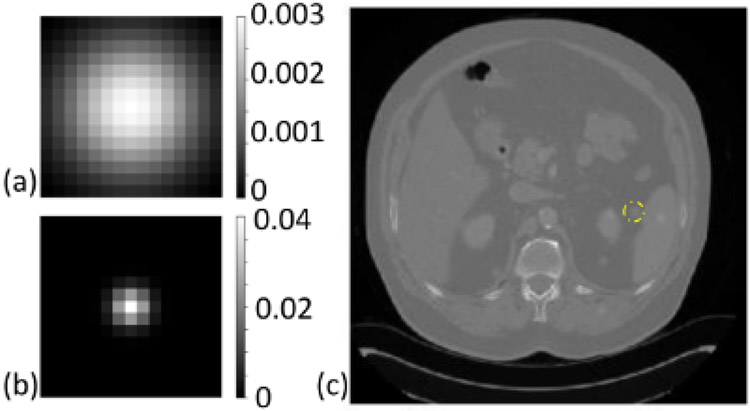
Two different task objects emulating a large low-contrast lesion and a small calcification (Figure 2) were inserted in the normal dose CT images in the testing set. For each image, 10 low-dose images were simulated with Poisson noise injection in projection data. The σ ranged in [0,4] for the high-contrast task and in [0,8] for the low-contrast task. Detectability indices were computed in the denoised estimates using the proposed sCNN and the RED-CNN. The relative detectability indices were computed by normalization to the corresponding RED-CNN detectability indices.
Figure 2:
The inserted task objects: (a) a flat Gaussian signal (standard deviation=4 pixels), (b) a sharp Gaussian signal (standard deviation=1 pixels). (c) Examples of normal dose CT images with task object insertions.
3. RESULTS
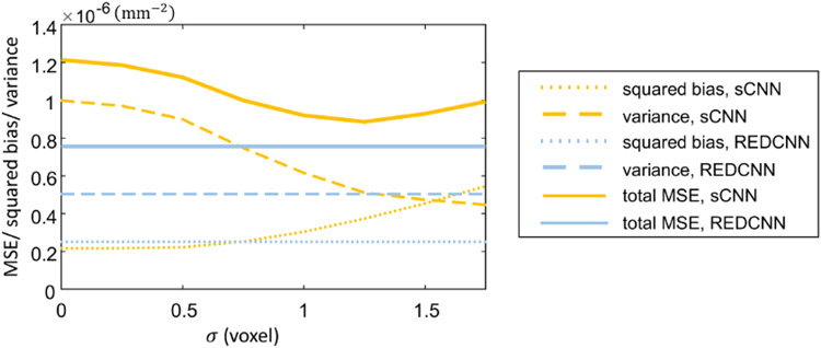
A representative sample of the reference normal-dose image, the simulated low-dose image, and the denoised images using RED-CNN and the proposed sCNN models are shown in Figure 3. Both the RED-CNN and sCNN results show significantly reduced noise and maintain most of the structures. Compared with the RED-CNN denoised image, the sCNN result with σ = 0 shows comparable image quality. Additionally, the sCNN provides further denoising ability with lower “resolution” for increasing σ values. Figure 4 displays three different mean-squared errors (MSE) including the total MSEs between denoised and the ground truth in solid lines, the MSE between the averaged denoised image among 100 noisy realizations for each test image in dotted lines, and the variance of denoise images with reference to the averaged denoised result in dashed lines. The total MSE is mathematically the sum of the squared bias and the variance. All MSEs are measured in a central 300-by-300 region-of-interest. The blue lines show the MSE measurements of the RED-CNN estimates, while the orange ones show those of the sCNN results. We observed that the squared bias increases monotonically with the sigma values, while the variance decreases. The total MSE of sCNN denoised estimates decreases with the increased σ until the turning point σ = 1.25. When compared with the REDCNN MSEs, the total MSE of sCNN is not lower, but the variance component can reach a lower level at the price of introduced bias. This is consistent with the visualization observation in Figure 3 and demonstrates that the proposed sCNN can establish a noise-bias trade-on with the proposed network structure.
Figure 3:
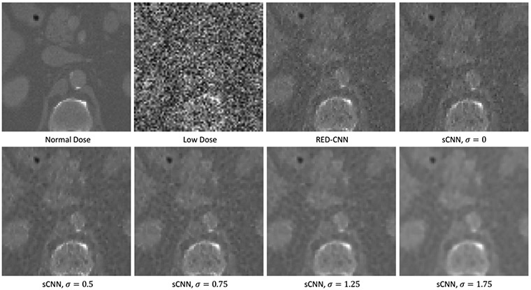
One example in the testing set. The normal dose image (ground truth), the simulated low-dose image, and the denoised images with the RED-CNN model or the proposed sCNN model at different resolution levels are displayed. All display windows are [0,0.03] mm−1
Figure 4:
Mean squared errors evaluations.
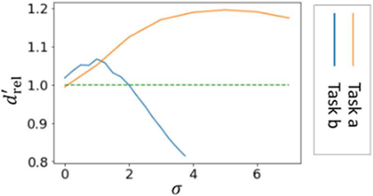
The average relative detectability indices are plotted in Figure 5 The task-based evaluation shows that with the sCNN model, the detectability is optimized at different σ values for the low-and high-frequency imaging tasks. Moreover, the optimized detectability is greater than the RED-CNN (green dotted line) which has no resolution control. The optimal σ of the low-frequency low-contrast imaging task is higher than the small high-contrast task. This is expected because the low-frequency imaging task is less sensitive to spatial resolution loss and benefits from additional noise reduction.
Figure 5:
Relative detectability indices of two imaging tasks with respective to σ at locations 1 (left) and 2 (right).
4. CONCLUSIONS AND DISCUSSION
In this work, we proposed a CNN for noise reduction in low-dose CT with spatial resolution control and evaluated the network performance with general quantitative metrics of MSE and task-based detectability. The results showed that the introduction of spatial resolution control provides controllability over how aggressively the noise reduction is applied. This allows for a personalized selection of the trade-off between the bias and the variance, and permits customization for specific diagnostic tasks. We expect that such controllability also yields an opportunity to investigate and control more general biases associated with machine learning methods with special attention to misrepresenting structures. A neural network with this kind of parameterization may permit tuning of the approach to both explore and limit the introduction of false features in a reconstruction. For example, a feature may be less likely to be false if presenting in both less and more aggressively applied noise reduction. Such questions and analyses are the subjects of ongoing efforts.
ACKNOWLEDGMENTS
This work is supported, in part, by NIH grants R01CA249538 and R01EB027127.
REFERENCES
- [1].Li Z, Yu L, Trzasko JD, Lake DS, Blezek DJ, Fletcher JG, McCollough CH, and Manduca A, “Adaptive nonlocal means filtering based on local noise level for CT denoising,” Medical Physics 41(1), 1–16 (2014). [DOI] [PubMed] [Google Scholar]
- [2].Dabov K, Foi R, Katkovnik V, and Egiazarian K, “BM3D image denoising with shape-adaptive principal component analysis,” Proc. Workshop on Signal Processing with Adaptive Sparse Structured Representations, 6 (2009). [Google Scholar]
- [3].Chen H, Zhang Y, Kalra MK, Lin F, Chen Y, Liao P, Zhou J, and Wang G, “Low-Dose CT With a Residual Encoder-Decoder Convolutional Neural Network,” IEEE Transactions on Medical Imaging 36, 2524–2535 (December 2017). [DOI] [PMC free article] [PubMed] [Google Scholar]
- [4].Gang GJ, Stayman JW, Ehtiati T, and Siewerdsen JH, “Task-driven image acquisition and reconstruction in cone-beam CT.,” Physics in medicine and biology 60(8), 3129–3150 (2015). [DOI] [PMC free article] [PubMed] [Google Scholar]
- [5].Gang GJ, Guo X, and Stayman JW, “Performance analysis for nonlinear tomographic data processing,” in [15th International Meeting on Fully Three-Dimensional Image Reconstruction in Radiology and Nuclear Medicine], Matej S and Metzler SD, eds., 124, SPIE (May 2019). [Google Scholar]
- [6].Kang E, Min J, and Ye JC, “A deep convolutional neural network using directional wavelets for low-dose X-ray CT reconstruction,” Medical Physics 44(10), e360–e375 (2017). [DOI] [PubMed] [Google Scholar]
- [7].Clark K, Vendt B, Smith K, Freymann J, Kirby J, Koppel P, Moore S, Phillips S, Maffitt D, Pringle M, Tarbox L, and Prior F, “The cancer imaging archive (TCIA): Maintaining and operating a public information repository,” Journal of Digital Imaging 26(6), 1045–1057 (2013). [DOI] [PMC free article] [PubMed] [Google Scholar]
- [8].Kingma DP and Ba JL, “Adam: A method for stochastic optimization,” 3rd International Conference on Learning Representations, ICLR 2015 - Conference Track Proceedings, 1–15 (2015). [Google Scholar]


