Baroclinic waves in the northern hemisphere of Mars as observed by the MRO Mars Climate Sounder and the MGS Thermal Emission Spectrometer

Abstract

The climatology of baroclinic waves in the northern hemisphere of Mars is investigated through analysis of observations by the infrared sounders on Mars Reconnaissance Orbiter (MRO) and Mars Global Surveyor (MGS). We focus on the lowest scale height above the surface, where the waves have a large impact on the Martian dust cycle. Profiles retrieved by the MRO Mars Climate Sounder (MCS) rarely reach the lower atmosphere at the season and location of interest. To fill this gap, we turn to observations in the MCS B1 channel (32 microns) when the instrument is viewing the surface. The signature of baroclinic waves appears in these data because of dust-related emission from the lower atmosphere and wave-induced variations of surface temperature. We supplement the MCS data with measurements of temperature at the 610-Pa pressure level from the MGS Thermal Emission Spectrometer (TES). Both data sets provide systematic coverage in latitude and longitude at two local times. Characteristics of baroclinic waves are derived through analysis of observations with a combined duration of about 8 Mars years. Basic results include least-squares solutions for wave amplitude and period at zonal wavenumber 1–3; the resolution is 4° in latitude and 14 solar days in time of observation. There is a strong similarity between the baroclinic waves observed by MCS and TES, which confirms the sensitivity of the MCS B1 channel to wave activity at pressures near 610 Pa. In all 8 Mars years, the baroclinic waves exhibit periodic transitions among modes with different zonal wavenumbers and a distinctive solstitial pause. Although the weather in each Mars year is unique in some respects, a composite of results from all years reveals a well-defined wave climatology. At each zonal wavenumber, large amplitudes are restricted to a pair of seasonal windows positioned symmetrically about the winter solstice. The wave-2 mode is strongest in early autumn and near the vernal equinox, whereas wave 3 is the dominant mode in mid-autumn and mid-winter, immediately before and after the solstitial pause. The interaction between baroclinic waves and dust storms is investigated through comparisons with spacecraft measurements of dust opacity. A strong wave-3 mode is often present during the initial growth phase of large, seasonal dust storms, which reflects the importance of wave-generated frontal dust storms in triggering these events. The wave-3 amplitude then decreases rapidly as the dust storm evolves; this occurs routinely in all Mars years considered here in connection with both mid-autumn “A” storms and mid-winter “C” storms. In some years A-storm suppression of the wave-3 mode marks the beginning of the solstitial pause. These results provide a basis for testing and development of Mars General Circulation Models as well as context for interpreting contemporaneous observations, such as spacecraft images of frontal and flushing dust storms.

1. Introduction

The terms ‘transient eddies’ and ‘transient waves’ are used in the Martian literature to refer to disturbances that arise from several types of instability. The subject of this paper is transient eddies at mid-to-high latitudes in the lowest scale height above the surface. Their location, seasonality, and strong poleward eddy heat flux imply that they arise from baroclinic instability (Lewis et al., 2016; Barnes et al., 2017). Hence, we refer to them as baroclinic waves. This type of wave travels eastward, is periodic in longitude with zonal wavenumber 1–3, and appears seasonally in both hemispheres of Mars. We limit discussion in this paper to the northern hemisphere, where baroclinic waves play an important role in the Martian dust cycle by initiating frontal and flushing dust storms during the autumn and winter seasons (Wang et al., 2005; Hinson et al., 2012). See Barnes et al. (2017) for a review of observations and modeling of baroclinic waves and a discussion of their influence on Martian weather and climate.

The Mars Climate Sounder (MCS) on Mars Reconnaissance Orbiter (MRO) is a nine-channel, infrared, filter radiometer that monitors the atmosphere in both limb- and surface-viewing geometries (McCleese et al., 2007; Kleinböhl et al., 2009). Both types of data provide daily global coverage at two local times. The primary function of MCS is limb sounding, and the resulting atmospheric profiles have had a major impact on many areas of atmospheric research (Barnes et al., 2017). However, there has been little progress to date in understanding the type of wave considered here, either from direct analysis of the retrieved temperatures or through data assimilation, as discussed in Section 2. This arises in part from the difficulty inherent to infrared limb sounding in the baroclinic zone where the waves reside. In addition, the opacity of the lower atmosphere is substantial at the season and location of interest, which severely limits the number of limb profiles that extend downward to pressures greater than 350 Pa (see Fig. 1, below).

As we show in this paper, surface-viewing observations in the MCS B1 channel (32 microns) are a valuable source of information about baroclinic waves. Through analysis of these data, we have derived a multi-year record of wave activity that fills the low-altitude gap in the MCS limb profiles and provides new insight into many aspects of wave behavior. The data are sufficient in both quality and quantity to construct a definitive climatology of baroclinic waves and to characterize their response to major dust storms.

There are two ways for baroclinic waves to influence the brightness temperature in the B1 channel. First, dust is the main atmospheric absorber at 32 microns (Kleinböhl et al., 2009); the waves modulate the temperature of the dust and its spatial distribution, imposing the signature of the waves on the atmospheric emission. Second, the atmosphere is relatively transparent at 32 microns, despite the dust, which allows the B1 channel to observe wave-induced variations in surface temperature. We don’t currently know the relative magnitude of the emission from the two sources, although we have inferred from observations above the CO₂ ice cap that the atmospheric component is appreciable (Section 5.2.1).

Our objectives do not require a detailed understanding of how the waves influence the 32-micron brightness temperature. However, it is essential to know the vertical location of the waves whose signature appears in these data. We answer this question through analysis of temperatures retrieved by the Thermal Emission Spectrometer (TES) on Mars Global Surveyor (MGS) (Smith et al., 2001; Smith, 2004); only the 610-Pa pressure level is considered here. Although TES data have been analyzed in previous investigations of baroclinic waves (e.g. Banfield et al., 2004; Lewis et al., 2016), we present the results in a way that provides additional insight and allows direct comparisons between TES and MCS. From the close resemblance between the waves observed by the two instruments, we conclude that the B1 channel is sensitive to waves at pressures greater than about 300 Pa.

We use standard conventions for timekeeping on Mars. The term “sol” denotes the mean solar day of 88,775 s. Local time is expressed in true solar hours (24 per sol). Seasons are defined by L_s, the angular position of Mars in its orbit about the Sun, with L_s ≡ 0° at the vernal equinox of the northern hemisphere. In assigning numbers to years we adopt the convention that Mars year 1 (MY1) began on 11 April 1955 (Clancy et al., 2000).

The paper is organized as follows. Section 2 reviews previous work and illustrates the limitations of MCS profiles for studies of dynamics near the surface. Section 3 describes the MCS and TES data used in this investigation. Section 4 introduces the method of analysis. Results from the two instruments are compared in Section 5. Section 5.1 gives an overview of MCS and TES results from 6 MYs. Section 5.2 explains how baroclinic waves are distinguished from measurement noise. Section 5.3 compares wave periods measured by MCS and TES. Section 5.4 looks closely at MCS and TES results from a single MY of observations by each instrument. Section 6 reports results drawn from the complete sets of MCS and TES observations; topics include baroclinic wave transitions, wave climatology, and dust-storm suppression of the wave-3 mode. Section 7 reviews our findings and discusses possible topics for future work. In Appendix A, we apply the same method of analysis to temperatures retrieved by MCS at the 610-Pa pressure level; the results are consistent with those derived from contemporaneous observations in the B1 channel, but their spatial coverage and general quality are not nearly as good. Appendix B provides access to supplementary data.

2. Background and motivation

This section provides a brief summary of the basic characteristics of baroclinic waves in the northern hemisphere. We limit the discussion to results derived from observations, including those obtained through data assimilation. See Barnes et al. (2017) for a comprehensive review of both observations and numerical simulations of baroclinic waves. This section also illustrates the limitations of MCS limb profiles for research in this area.

The Viking Landers monitored the atmosphere of Mars at two locations in the northern hemisphere, providing a multi-year record of pressure and temperature along with more limited measurements of winds. This led to numerous advances in our understanding of Martian weather and climate (Zurek et al., 1992). In particular, eastward-traveling baroclinic waves were observed for the first time (Ryan et al., 1978; Barnes, 1980, 1981; Ryan and Sharman, 1981; Leovy et al., 1985), confirming predictions by numerical models (Leovy and Mintz, 1969). The waves appear in autumn and winter with typical periods of 2–8 sols and an amplitude in surface pressure of a few percent. Amplitudes are much larger at 48°N (Lander 2) than at 22°N (Lander 1). Subsequent missions have shown that the waves have a discernible effect on surface pressure at 4.5°S in Gale Crater (Haberle et al., 2018) and at 4.5°N in Elysium Planitia (Banfield et al., 2020b).

The MGS TES sounded the atmosphere of Mars from summer of MY24 through spring of MY27 (Smith et al., 2001; Smith, 2004). Temperature profiles retrieved from nadir observations have a vertical resolution of about 10 km and provide complete global coverage at two local times. This space-time coverage is favorable for investigations of transient eddies, and much of what is known about this subject derives from the TES data. After Wilson et al. (2002) reported initial results from northern autumn and winter of MY24, Banfield et al. (2004) methodically analyzed TES data from MY24 and 25, solving for the amplitude, period, and zonal wavenumber of the transient eddies and mapping their three-dimensional spatial structure and seasonal evolution in both the northern and southern hemispheres. Subsequent analyses of TES profiles extended the survey of eddy activity in the northern hemisphere through MY26 (Wang, 2007; Wang et al., 2013). Rather than attempting to synthesize the results from these studies, we summarize basic properties of the transient eddies in the context of subsequent work by Lewis et al. (2016), especially as it applies to low-altitude baroclinic waves.

Lewis et al. (2016) investigated the ‘winter weather’ on Mars through data assimilation, using TES retrievals of temperature and dust opacity to guide a General Circulation Model (GCM). The reanalysis relies on the simulated general circulation and the model physics to determine the vertical structure of the baroclinic waves, which is not fully resolved by TES. We consider only the results in the northern hemisphere. The baroclinic waves have zonal wavenumbers of 1–3. The temperature field of both the wave-1 and wave-2 modes has a large amplitude at the surface, a minimum at a pressure of about 200 Pa, and a local maximum at about 20 Pa; the temperature field of wave-3 mode is largely confined to pressures exceeding 200 Pa. The amplitude is largest in early-to-mid autumn (L_s = 180–240°) and mid-to-late winter (L_s = 300–360°) near the edge of the seasonal CO₂ ice cap. In all 3 MYs observed by TES, the baroclinic waves subside near the winter solstice. This “solstitial pause” is apparent only at pressures greater than about 300 Pa, owing to the presence of a different type of transient eddy at higher altitudes in late autumn and early winter. The solstitial pause has a significant impact on the seasonal dust cycle: frontal and flushing dust storms, which are initiated by baroclinic waves, cease at about L_s = 240° and do not resume until after about L_s = 300° (Wang et al., 2005; Wang, 2007; Wang and Richardson, 2015).

Greybush et al. (2019) used a different type of data assimilation in a similar investigation of baroclinic waves at low altitudes. In this approach, the output from the reanalysis is a 16-member ensemble, which provides information about the reliability of the results: confidence increases as the ensemble spread decreases. When applied to TES temperature profiles, there is little difference among the members of the ensemble, and the ensemble mean closely resembles the results obtained by Lewis et al. (2016). However, similar reanalysis of MCS temperature profiles yielded mixed results. The ensemble does not converge consistently, owing to the scarcity of successful retrievals at pressures exceeding 350 Pa, as discussed below. This implies that the information contained in the MCS profiles (version 5) is not sufficient to support a comprehensive investigation of wave activity near the surface.

MGS radio occultation (RO) profiles of temperature and geopotential height provide additional information about baroclinic waves (Hinson and Wilson, 2002; Hinson, 2006; Hinson and Wang, 2010; Hinson et al., 2012). In particular, the vertical structure of the waves can be determined with sub-kilometer resolution. Fig. 1 shows three examples. In each case, the amplitude in temperature is largest at about 600 Pa and it decreases rapidly at lower pressures. This type of wave structure is largely inaccessible to MCS limb sounding. Among the 100,000 profiles available at mid-to-high northern latitudes during L_s = 180–360° of MY30, fewer than 20% reach pressures greater than 350 Pa, as shown in Fig. 1.

Figure 1:

Lower abscissa: Vertical structure of baroclinic waves derived from RO temperature profiles (Hinson, 2006; Hinson and Wang, 2010). Results are shown for (orange) a wave-1 mode with a period of 6.9 sols at 66°N in autumn (L_s =204–212°) of MY27; (light blue) a wave-2 mode with a period of 3.0 sols at 69°N in autumn (L_s =190–200°) of MY26; and (dark blue) a wave-3 mode with a period of 2.3 sols at 64°N in winter (L_s = 316–334°) of MY25. Upper abscissa: (black) fraction of MCS profiles that reaches a given pressure level at the season and location where baroclinic waves appear. Dots mark the standard pressure levels in the MCS retrievals.

The scarcity of MCS profiles at low altitudes is a serious impediment to studies of baroclinic waves. We illustrate this point in Appendix A by extracting samples of temperature at 610 Pa from 1 MY of MCS profiles and using the procedure described in Section 4 to search for waves. (Initial results from a similar effort were reported recently by Banfield et al. (2020a).) This yielded some tantalizing results, but there is a major gap in coverage throughout polar night and extending well into the surrounding baroclinic zone. The results from limb sounding are not sufficient to meet our objectives, which led us to consider another type of MCS observation.

3. Observations

This investigation relies on data from two infrared sounders, the MRO MCS and the MGS TES. The data sets have similar coverage in longitude, latitude, and local time. There is no overlap in atmospheric measurements by the two instruments.

3.1. The MRO Mars Climate Sounder

We examined MCS data acquired when the instrument was pointed at the surface and found that the B1 channel is the best source of information about baroclinic waves in the northern hemisphere. However, other channels may be needed when we extend the analysis to the southern hemisphere, where the surface pressure is generally smaller than in the north.

The observations used here come from Reduced Data Records (RDRs) stored at the Atmospheres Node of the NASA Planetary Data System (PDS). We consider only data acquired in a uniform viewing geometry with MCS pointed in the forward direction (178° < azimuth < 182°) and viewing the surface at an emission angle of about 60° (118° < elevation < 123°). In addition, we exclude any observation performed under abnormal conditions, such as when the spacecraft was rolling or when MCS was safing, safed, freezing, frozen, dumping, or moving (as defined in the PDS documentation for the RDRs).

The information extracted from the RDRs includes the calibrated B1 radiance, the time of observation (UTC), and the longitude, latitude, and local time at the observation point on the surface of Mars (based on reconstructions of spacecraft position and MCS pointing direction). We computed L_s for each data sample using classical orbital elements for Mars. Observations that meet all criteria mentioned above are obtained routinely as part of the standard MCS observing sequence (McCleese et al., 2007), providing regular coverage of both the dayside and the nightside as shown in Fig. 2.

Figure 2:

Spatial coverage of MCS surface observations from 13 consecutive orbits (about 1 sol) at L_s =25° of MY30. The local time is about 15 h for observations on the dayside (light blue) and about 3 h for observations on the nightside (dark blue).

We used radiances from detectors B1–10, B1–11 (the middle detector), and B1–12; the other 18 detectors of the B1 channel are ignored. The brightness temperature is computed from the average radiance in these three detectors using the inverse Planck function for the central wavenumber of detector B-11 (317.788 cm⁻¹). For example, Fig. 3 shows the variations of brightness temperature with latitude for the observations in Fig. 2. Atmospheric gases are transparent at 32 microns, so the emission comes primarily from the surface with a smaller contribution from atmospheric dust. Fig. 3 has several notable features. First, there is a large day-night temperature difference (about 80 K) at low latitudes. Second, spatial variations in surface thermal inertial cause substantial zonal variations in nightside temperature at latitudes south of 50°N. Third, there is a strong meridional gradient of brightness temperature at high latitudes, particularly on the dayside, where the temperature decreases from about 225 K at 60°N to less than 170 K at 70°N. Finally, the bimodal temperature distribution at latitudes north of about 70°N is a consequence of zonal variations in the distribution of CO₂ ice (Calvin et al., 2015). As we show in Section 5.4 (Fig. 11), a baroclinic wave is present at the time of these observations, with a zonal wavenumber of 2 and an amplitude of 2–3 K at 60–75°N.

Figure 3:

Samples of 32-micron brightness temperature for the observations in Fig. 2. Dayside (light blue) and nightside (dark blue) temperatures converge at the pole but differ substantially at mid-to-low latitudes. These measurements are from early spring (L_s = 25°) of MY30.

We computed the zonal-mean surface temperature at a local time of 15 h from B1 measurements such as those in Fig. 3. The results provide context for interpreting some aspects of the wave measurements. In particular, the 150-K contour gives the approximate location of the edge of the CO₂ ice cap. (See Figs. 6–8, below.)

Although it is not obvious from Fig. 3, the B1 channel also contains valuable information about baroclinic waves at pressures greater than 300 Pa. Two aspects of the results support the conclusions about the identity of the wave and its vertical location: (1) the presence of a deep solstitial pause, as discussed in Sections 5.1 and 6.2; and (2) the strong resemblance to baroclinic waves observed by TES at 610 Pa, as discussed in Sections 5.3, 5.4, and 6.2. Results derived through analysis of MCS temperature profiles also support this conclusion, as discussed in Appendix A.

The MCS measurements considered here extend from L_s = 329° of MY28 through L_s = 90° of MY34. There were no planet-enshrouding dust storms (PEDS) during this period.

3.2. The MGS Thermal Emission Spectrometer

As part of this investigation we also analyzed temperatures retrieved from TES nadir measurements (Conrath et al., 2000; Smith, 2004). Like MCS, TES provided daily global coverage at two local times, but the TES coverage differs in several respects from that shown in Fig. 2. First, profiles were obtained more frequently by TES, which reduces the separation in latitude between successive measurements. Second, MGS completed 12.6 orbits per sol, as compared with 13.2 for MRO. Finally, TES sampled local times of about 2 and 14 h, 1 h earlier than MCS. None of these differences is important in the context of this investigation.

TES nadir profiles extend from the surface to the 10-Pa pressure level; the vertical resolution is about 10 km. For present purposes it is sufficient to consider only temperature measurements at the 610-Pa pressure level, which is well aligned with the near-surface peak in wave amplitude (see Fig. 1). In the autumn and winter seasons, the surface pressure in the northern hemisphere generally exceeds 610 Pa at mid-to-high latitudes, where the wave amplitude is largest.

The TES measurements used in this investigation extend from L_s = 141° of MY24 through L_s = 72° of MY27. One PEDS occurred within this period, in autumn of MY25.

4. Method of analysis

Several methods of analysis have been used in previous investigations of baroclinic waves, as reviewed by Barnes et al. (2017). We chose a least-squares method for several reasons. First, it can be applied directly to data with irregular sample spacing in longitude and time of observation, which makes it easy to combine data from the dayside and the nightside. In addition, each data sample can be weighted according to its accuracy; equal weights are used here, but we may assign different weights to data from the dayside and the nightside in future work. Finally, the method can be applied directly to data sets with occasional missing samples; no special treatment, such as interpolation, is required.

The least-squares method of analysis used here has been applied successfully in several previous investigations of baroclinic waves (Hinson, 2006; Hinson and Wang, 2010; Hinson et al., 2012). It is designed for the study of waves that are synoptic in scale and periodic in longitude. This section explains how it is applied to the MCS and TES datasets. See Hinson et al. (2012) for a more complete description of the method.

The data are separated into bins by latitude and time of observation (UTC); each bin contains data with complete longitude coverage from both the dayside and the nightside. Several factors influence the choice of bin size. The meridional dimension is 4°, large enough to include many samples but small enough to resolve the meridional structure of the waves (see Section 5.4). We set the bin size in the time dimension to 14 sols. This choice affects the results in two ways. First, it places an upper limit of 14 sols on the period of the waves that can be detected reliably. The waves considered here have typical periods of 2–10 sols (see Sections 5.3 and 6.2), comfortably within this limit. Second, it determines the time resolution in measurements of the seasonal evolution of the waves. The sensitivity of the results to the choice of bin size is discussed in Sections 6.1 and 6.2.

As shown below in Fig. 13, there are occasional gaps in the data, which arise primarily from interruptions in spacecraft operations. Apart from these gaps, the average number of samples per bin is 1100 for MCS and 6800 for TES.

The bin spacing is smaller than the bin size, in order to ensure that the choice of bin centers does not obscure useful information. Specifically, the bins overlap by 50% in latitude, with bin centers on the even-numbered parallels. The overlap in time of observation is more than 50%, with bin centers separated by 2° in L_s (roughly 4 sols). The bin centers are specified in terms of L_s rather than sol number for two reasons. First, L_s is a more familiar way of describing time of year on Mars. Second, bins centered in L_s are convenient for comparing results from different years, whereas sol number is problematic in that the number of sols in 1 MY is not an integer.

Extraneous components of surface emission are removed from the data within each bin; the procedure is applied separately to observations from the dayside and the nightside. First, we exclude MCS measurements where the brightness temperature is anomalously cold (< 135 K); this reduces the noise floor but has no appreciable effect on solutions for wave parameters. Second, the seasonal trend is removed by fitting a line to samples of brightness temperature versus L_s and subtracting it from the data. Third, the meridional trend is removed in the same manner. Finally, the albedo and thermal inertia of Mars are nonuniform, which results in large spatial variations of brightness temperature in measurements at fixed local time, especially at night (Fig. 3). This component of surface emission is greatly reduced by fitting stationary zonal harmonics through wavenumber 4 to samples of brightness temperature versus longitude and subtracting them from the data.

After removing the extraneous surface emission, we combine the data from the dayside and the nightside and search for baroclinic waves at zonal wavenumber 1–4. Data from each bin are analyzed independently. Results include least-squares solutions for the amplitude and period of the strongest mode at each wavenumber. As in previous studies, eastward-traveling modes with wavenumber 1–3 have large amplitudes at some latitudes and seasons. Wave 4 is also detected by both TES and MCS, but it rarely exceeds the noise level (see Fig. 10, below). The results from all bins were assembled into a database that spans nearly 3 MYs for TES and more than 5 MYs for MCS.

We illustrate the method of analysis and the quality of the MCS data by showing results from a single bin. The data can be viewed in two ways. Fig. 4 shows results in the frequency domain. The spectrum is dominated by an eastward-traveling wave-3 mode with a period of 2.1 sols and a zonal phase speed of 56° sol⁻¹. The full width at half maximum of the main peak is 0.07 sol⁻¹, which corresponds to the spectral resolution of a bin with a duration of 14 sols. Hence, over this time span the wave is indistinguishable from a pure sinusoid.

Figure 4:

Least-squares spectrum showing results from a single bin centered at 48°N and L_s = 226° of MY29. The spectrum is dominated by a wave-3 mode with an amplitude of 4.5 K and a frequency of 0.47 sol⁻¹ (a period of 2.1 sols). The frequency range is appropriate for satellite observations twice per orbit (Salby, 1982). The spectrum is oversampled for clarity. Secondary peaks offset by ±0.107 sol⁻¹ from the primary peak result from use of a rectangular window function.

Fig. 5 shows the results from the same bin in the longitude-time domain, where the least-squares solution for the wave is compared with data from both the dayside and the nightside. The standard deviation of the fit is 3.3 K, as compared with a wave amplitude of 4.5 K. In this example, the wave is unusually strong but the noise is typical of the MCS measurements. Independent analysis of data from the dayside and the nightside yields solutions for wave properties that differ by only 0.4 K in amplitude and 0.01 sol⁻¹ in period from the solution derived from the combined observations.

Figure 5:

Data from Fig. 4 as viewed in the longitude-time domain. The horizontal axis is longitude in a frame moving eastward at the zonal phase speed of the wave (56° sol⁻¹). Light and dark blue dots denote data from the dayside and nightside, respectively. The black line is the the least-squares fit to the data.

5. Comparisons of results from MCS and TES

The results in this section illustrate the quality of the MCS observations and demonstrate that MCS and TES give consistent characterizations of baroclinic waves. Section 5.1 surveys the data from both instruments. Section 5.2 describes the measurement noise and explains how baroclinic waves are identified. Section 5.3 examines the dependence of wave period on zonal wavenumber. Section 5.4 compares TES results from MY26 with MCS results from MY30.

5.1. RSS amplitude

Fig. 6 provides a compact summary of observations from 6 MY. The quantity displayed is the RSS amplitude, which is obtained by summing the squared amplitudes at waves 1–3 and taking the square root. In the discussion that follows, we consider first the distribution in latitude and season of the baroclinic waves. We then describe a type of low-latitude noise that appears only in the MCS observations.

Figure 6:

RSS amplitude of baroclinic waves at zonal wavenumber 1–3. Each panel shows 1 MY of measurements beginning at the summer solstice (L_s =90°). The label at the lower left is the MY at the winter solstice (L_s =270°). TES results are shown in (A) and (B); MCS results are shown in (C)–(F). White bands denote data gaps. Panels (C)–(F) show the 150-K contour (white) of zonal-mean, daytime surface temperature, which tracks the edge of the CO₂ ice cap. Note that different color bars are used for results from TES and MCS.

Baroclinic waves appear in the TES observations at latitudes north of about 40°N. Within that region, the general pattern of wave activity is similar in all 6 MYs shown in Fig. 6. The RSS amplitude is largest in early-to-mid autumn (L_s = 180–240°) and mid-to-late winter (L_s = 300–360°) near the edge of the seasonal CO₂ ice cap. There is a distinctive decrease in amplitude near the winter solstice in all MYs shown here. This feature is the solstitial pause (Lewis et al., 2016), which occurs only at pressures greater than about 300 Pa, as discussed in Section 2. Its presence in the MCS observations indicates that the B1 channel is sensitive to wave activity near the surface.

The RSS amplitude exhibits strong, transitory peaks that arise from modes with different zonal wavenumbers, as discussed in Section 6.1. Their timing and magnitude vary from year to year. This is apparent in the large differences between pre-solstice activity in MY29 and 31, and between post-solstice activity in MY26 and 30. (In this and all subsequent figures, we refer to each panel by the year number at the winter solstice.)

There is an important difference between the two types of observation in Fig. 6. TES measures the wave amplitude in physical temperature at 610 Pa. In contrast, MCS measures its amplitude in 32-micron brightness temperature, which depends not only on the amplitude in physical temperature but also on the emissivity of the lower atmosphere and the magnitude of the wave-induced variations in surface temperature. A comparison of the RSS amplitudes in Fig. 6 shows that the wave amplitude in 32-micron brightness temperature is about half as large as its amplitude in physical temperature.

Fig. 6 shows that MCS is considerably noisier than TES at latitudes south of 40°N, particularly in a prominent band at 20–30°N, which repeats from year to year. The source of this noise is discussed in the next section.

5.2. Measurement noise

The properties of the measurement noise are considerably different for MCS and TES. This section explains the procedure used to distinguish atmospheric waves from measurement noise in each dataset.

5.2.1. MCS

The MCS noise is characterized as follows. Each bin is analyzed separately. We subtract the best fit at each zonal wavenumber from the data (dayside and nightside combined) and then compute the standard deviation σ_n of the remaining noise; for example, σ_n is 3.3 K for the example in Fig. 5. Fig. 7 shows the resulting map of MCS noise in MY30. The figure also shows several contours of zonal-mean surface temperature at a local time of 15 h. Results from other MYs look essentially the same (not shown).

Figure 7:

Variations of MCS noise σ_n with latitude and season in MY30 (color). White lines show contours of zonal-mean, daytime surface temperature. Contours range from 150 K to 240 K with a spacing of 15 K. The arrow indicates the midpoint of the largest frontal dust storm in MY30 (Wang and Richardson, 2015), which coincides with a notable enhancement of σ_n.

The CO₂ ice cap causes σ_n to vary strongly with both latitude and season. Its value ranges from about 1 K above the ice, where the surface temperature is nearly uniform, to more than 5 K near the edge of the receding CO₂ ice cap. This cap-edge noise is associated with the steep north-south gradient of dayside surface temperature (Fig. 3), which is difficult to remove from the data.

Wang and Richardson (2015) have identified and cataloged the distribution and evolution of large dust storms through analysis of wide-angle images from the MGS Mars Orbiter Camera (MOC) and the MRO Mars Color Imager (MARCI). A comparison of their results with the noise map in Fig. 7 shows that frontal dust storms are responsible for some of the variability of σ_n. For example, large frontal dust storms occurred simultaneously in Acidalia and Utopia at L_s = 330.0–336.6° of MY30. The midpoint of this event is labeled by a white arrow in Fig. 7. It coincides with a brief enhancement of σ_n that extends in latitude from the tropics to the CO₂ ice cap. This pair of storms influenced the 32-micron emission by injecting dust into the lower atmosphere, which increases the emissivity, and by altering the surface temperature.

Two criteria are used to distinguish waves from noise in the MCS observations, as illustrated in Fig. 8. The first depends on the signal-to-noise ratio (SNR), defined as the ratio of the wave amplitude to the value of σ_n in the same bin. We attribute SNRs that exceed 0.35 to baroclinic waves (Fig. 8A); SNRs that fall below this threshold are assumed to be noise (Fig. 8B). This approach works well in that the period is generally independent of latitude in Fig. 8A, as expected for large-scale waves. We chose a threshold of 0.35 after reviewing results at zonal wavenumber 1–3 in all MYs; the same threshold is used for all results reported here. Fig. 8A also shows that the wave period varies significantly with L_s, as discussed in Sections 5.4 and 6.2.

Figure 8:

MCS results at zonal wavenumber 2 in MY30, showing the wave period (A) in all bins where the SNR exceeds 0.35, and (B) in bins excluded from (A). The color bar is logarithmic. The black line in (A) separates atmospheric waves (to the north) from measurement noise (to the south). The white line in (A) is the 150-K contour of zonal-mean, daytime surface temperature, which tracks the edge of the CO₂ ice cap.

Baroclinic waves are detected above the CO₂ ice cap (Fig. 8A). This must be a consequence of emission from the atmosphere, because exchanges of latent heat between the atmosphere and the ice greatly reduce the magnitude of any wave-induced variations of surface temperature. A comparable amount of atmospheric emission is expected to be present at latitudes where ice is absent.

The results at low latitudes in Fig. 8A are probably false positives for two reasons. First, the period is essentially constant and uncorrelated with the wave period at mid-to-high latitudes. Second, the predominant period at low latitudes, about 16/3 sols, is a harmonic of the repeat cycle of the MRO orbit (211 orbits in 16 sols, with an offset of about 0.5° in longitude between successive cycles). It appears that the sampling pattern of the in-track observations causes false positives in bins that contain large horizontal gradients in surface temperature. For example, this occurs in nighttime measurements at low latitudes in connection with spatial variations of surface thermal inertia.

We use an empirically derived latitude boundary (Fig. 8A) to separate these false positives (south of the boundary) from real atmospheric waves (north of the boundary). At wave 2, the latitude boundary Φ_b is defined as:

$${\Phi }_b=85°-40°\text{cos}\left[\left(L_s-270°\right)\pi /450°\right].$$ (1)

The preceding formula is also used for waves 1 and 4. However, the wave-3 mode extends to lower latitudes, as discussed in Section 5.4, so that a different boundary is required:

$${\Phi }_b=85°-50°\text{cos}\left[\left(L_s-270°\right)\pi /360°\right].$$ (2)

Both boundaries are shown below in Figs. 11 and 12. We demonstrate the effectiveness of these boundaries in Section 5.3.

5.2.2. TES

The SNR threshold is essential for interpreting the MCS data, where σ_n varies strongly with both latitude and L_s but repeats closely from year to year. The reverse is true for TES — the noise is independent of latitude but it increases noticeably from year to year. For TES, it is easier to compare results from different MYs when noise is removed through use of an amplitude threshold.

We selected a threshold of 1.7 K after reviewing TES wave measurements from MY24–26 at zonal wavenumber 1–4. Fig. 9 shows representative results, analogous to those in Fig. 8. The procedure used to separate baroclinic waves (Fig. 9A) from noise (Fig. 9B) is reasonably effective. We used the same threshold for all zonal wavenumbers in all MYs.

Figure 9:

TES results at zonal wavenumber 2 in MY26, showing the wave period (A) in all bins where the amplitude exceeds 1.7 K, and (B) in bins excluded from (A). The format is the same as in Fig. 8. Gray shading indicates data gaps.

The noise observed by MCS at low latitudes in Figs. 6 and 8 arises from surface emission. This type of noise is absent from the corresponding TES results for the following reason. Emission from the surface is removed from TES data prior to profile retrieval, using observations on either side of the 15-micron CO₂ absorption band (Conrath et al., 2000). This is especially important in sounding the atmosphere at the 610-Pa pressure level, which involves observations at wavelengths that include a significant amount of surface emission. The calibration works well enough to prevent surface artifacts from appearing in the TES results reported here.

The TES data are affected by systematic radiometric errors that grew in magnitude as the spacecraft and instrument aged (Pankine, 2015). Their impact on nadir measurements is largest where the surface is cold, at night and at high latitudes in autumn and winter. These radiometric errors may be responsible for the year-to-year increase in the noise level of the TES wave measurements. Nonetheless, the results from MY26 are similar in character to those obtained in all other MYs (see Figs. 6, 13, and 17), which implies that our method of analysis yields reliable results throughout the MGS Mission.

5.3. Statistics of wave period

Baroclinic waves have a period that depends on the zonal wavenumber (Banfield et al., 2004), as shown in Fig. 10. The TES measurements (Fig. 10A–10D) and the MCS measurements at mid-to-high latitudes (Fig. 10E–10H) are dominated by baroclinic waves, and there is a close resemblance between the results from the two instruments at each wavenumber. Conversely, the dominant period in the MCS histograms at low latitudes is 16/3 sols at all wavenumbers (Fig. 10I–10L); a comparison with the results in Fig. 10A–10H confirms that it is not associated with the baroclinic waves. The results in Fig. 10I–10L also demonstrate that the latitude boundaries defined in Section 5.2.1 are effective at eliminating the 16/3-sol noise from MCS measurements of wave period.

Figure 10:

(A)–(D) Histograms of wave period for TES observations where the amplitude exceeds 1.7 K. This includes all TES results except those from L_s =180–270° of MY25, which are affected by a PEDS. (E)–(L) Corresponding results from all MCS observations (MY28–33) where the SNR exceeds 0.35. MCS results are shown separately for observations (E)–(H) to the north and (I)–(L) to the south of the latitude boundaries discussed in Section 5.2.1. A period of 16/3 sols is marked by a vertical white line in (J)–(L). A different vertical axis is used in each row.

For both TES and MCS, there are relatively few bins where the wave-4 amplitude exceeds the noise level, as shown in Fig. 10D and 10H. The peak amplitude at waves 1–3 is 8–10 K for TES and 4–5 K for MCS; the peak amplitude at wave 4 is about three times smaller for both instruments. In the remainder of this paper we focus primarily on results for waves 1–3.

Several basic properties of the baroclinic waves are apparent in Fig. 10. For TES, the most common value of wave period is 6.6 sols at wave 1, 3.5 sols at wave 2, and 2.3 sols at wave 3 (Fig. 10A–10C). The corresponding numbers for MCS are 7.2, 3.5, and 2.3 sols (Fig. 10E–10G). The standard deviation of wave period is essentially the same for TES and MCS: 2.9 sols at wave 1, 1.7 sols at wave 2, and 0.8 sols at wave 3. Hence, the distribution becomes narrower as the zonal wavenumber increases. Another notable aspect of the results in Fig. 10 is the presence of significant activity with a period of about 2.3 sols at all zonal wavenumbers, including wave 4; we return to this point in Section 6.2. These solutions for the wave period are consistent with results derived previously from Viking Lander pressure measurements (Barnes, 1980, 1981), TES measurements of atmospheric temperature (Banfield et al., 2004), and RO measurements of geopotential height (Hinson, 2006).

5.4. MY26 and 30

This section compares 1 MY of wave observations by MCS and TES. We examine both the amplitude and period at each zonal wavenumber.

We begin with wave amplitude. Fig. 11A–11C shows the amplitude at zonal wavenumbers 1–3 observed by MCS in MY30. Wave activity was detected by MCS between the fall equinox and early spring. There are strong peaks in amplitude that alternate among the three zonal wavenumbers, and their location in latitude evolves in response to the seasonal expansion and contraction of CO₂ ice cap. Wave-2 peaks appear near the equinoxes at relatively high latitudes (Fig. 11B). Wave-3 peaks appear closer to the winter solstice at lower latitudes (Fig. 11C). There is a strong wave-1 peak in mid-autumn (Fig. 11A), but the amplitude at wave 1 is relatively small after the winter solstice. Banded structure at mid-to-low latitudes (to the south of the curving line in each panel) is 16/3-sol noise, as discussed in Sections 5.2 and 5.3. As in Fig. 10, this type of noise is strongest at wave 3 and negligible at wave 1.

Figure 11:

(A)-(C) MCS measurements of wave amplitude in MY30. Results are shown only in bins where the SNR exceeds 0.35. The black line in each panel is an empirically derived boundary (defined in Section 5.2.1) that separates reliable measurements of baroclinic waves at mid-to-high latitudes from surface-related noise at low latitudes. (D)-(F) TES measurements of wave amplitude in MY26. Results are shown only in bins where the amplitude exceeds 1.7 K. Gray shading indicates data gaps. Fig. 12 shows the corresponding measurements of wave period.

Fig. 11D–11F show the wave amplitudes observed by TES in MY26. The general pattern of activity is similar to what was observed by MCS in MY30, with isolated peaks in amplitude at each zonal wavenumber and a pattern of wave activity that shifts from higher latitudes near the equinoxes to lower latitudes near the winter solstice. The timing of the peaks is different in the two MYs, particularly after the winter solstice at wavenumbers 2 and 3.

Lewis et al. (2016) used a different approach (data assimilation) to characterize the baroclinic waves in the TES data, as discussed in Section 2. Their Fig. 9 summarizes wave activity at 1.8 km above ground level for each zonal wavenumber. In MY26, the timing, latitude, and magnitude of the peaks in wave amplitude are essentially the same as those derived here (Fig. 11D–11F). There is equally good agreement in MY24 and 25 (not shown).

Fig. 12 shows the corresponding measurements of wave period by MCS and TES. As in Fig. 11 there is a strong resemblance between the results from the two instruments. When the amplitude is large, the meridional extent of the waves is 20–40° and the period is independent of latitude. The periods associated with the largest amplitudes are the same as in Fig. 10. When the amplitude is relatively small, the behavior is sometimes more complex. In particular, two modes with the same wavenumber but different periods can appear simultaneously in adjacent latitude bands. For example, this occurred at wave 2 in mid-autumn (L_s = 210–225°) of both MY30 and 26 (Fig. 11B and 11E, respectively).

Figure 12:

(A)-(C) MCS measurements of wave period in MY30. Results are shown only in bins where the SNR exceeds 0.35. The black line in each panel is an empirically derived boundary (defined in Section 5.2.1) that separates reliable measurements of baroclinic waves at mid-to-high latitudes from surface-related noise at low latitudes. (D)-(F) TES measurements of wave period in MY26. Results are shown only in bins where the amplitude exceeds 1.7 K. Gray shading indicates data gaps. The color bar is logarithmic rather than linear so that the colors are distributed more evenly among the three zonal wavenumbers. Fig. 11 shows the corresponding measurements of wave amplitude.

In Fig. 12 the wave period evolves distinctively with season at each zonal wavenumber. The patterns are similar in MY26 and 30. The magnitude of the seasonal variations is smallest at wave 3, where the period remains within a relatively narrow range, and largest at wave 1. See Section 5.3 for further discussion.

6. Wave evolution, variability, and climatology

A high-quality record of baroclinic wave activity is now available from TES and MCS observations with a combined coverage of 8 MY. In this section, we use the results from both instruments to investigate the seasonal evolution of the wave modes, the year-to-year variability, the wave climatology, and the interdependence of waves and dust storms.

6.1. Baroclinic wave transitions

A compact summary of activity at each zonal wavenumber can be obtained by averaging the amplitude with respect to latitude and plotting the results versus L_s. The average is computed within a fixed, 30° latitude band where the amplitude is largest. From inspection of Fig. 11, we selected latitude bands of 40–70°N for wave 3 and 50–80°N for waves 1 and 2. All bins are included in the average (regardless of SNR or amplitude) so that the average amplitude includes a noise floor. The results appear in Fig. 13. Wave activity in autumn of MY25 was strongly affected by a PEDS. For that reason observations from L_s = 180–270° of MY25 are excluded from the wave climatology in Section 6.2.

Figure 13:

Seasonal evolution of the average amplitude at (orange) wave 1, (light blue) wave 2, and (dark blue) wave 3 in (A) MY24–26, (B) MY28–30, and (C) MY31–33. Gray bands denote data gaps. The horizontal bar in (A) identifies a period when wave activity was strongly affected by a PEDS. As in Figs. 6 and 11, different amplitude scales are used for TES and MCS. See Appendix B for a link to the data shown in this figure.

During mid-autumn and mid-winter, when the waves are most active, there is a succession of strong, transitory peaks in wave amplitude that alternate among modes with different zonal wavenumbers. Peak amplitudes are typically 4–7 K for TES and 2–4 K for MCS. Some modes persist for as long as 40 sols. These baroclinic wave transitions occur in all MYs covered by Fig. 13; they are a basic attribute of the wave dynamics.

In Fig. 13, the growth and decay of an individual wave mode is reasonably well resolved with the bin size used here (14 sols or about 8° of L_s), as required for a reliable representation of the baroclinic wave transitions. However, there are a few exceptions. The amplitude of the wave-3 mode decreases by a factor of three in only 14 sols at both L_s = 220° of MY32 and L_s = 325° of MY33. This appears to be a consequence of dust-storm suppression of the wave-3 mode, as discussed in Section 6.3.

There is considerable year-to-year variability in the detailed properties of the various wave modes. For example, a strong wave-3 mode appears in mid-autumn (near L_s = 225°) of both MY24 and 29, but the wave-3 mode is insignificant throughout autumn of MY33. In addition to this variability, there are patterns of behavior that repeat from year to year, as discussed in the next section.

6.2. Climatology

Fig. 14 shows the MCS results from Fig. 13 in a different format. Several patterns are immediately apparent. In all 5 MYs, large wave amplitudes occur in early-to-mid autumn and mid-to-late winter, on either side of a deep solstitial pause. Furthermore, each mode is most active within two, 45° windows of L_s, one in autumn and one in winter. In autumn, wave 2 usually precedes wave 3 with wave 1 interspersed. In winter, the sequence is reversed. Within this climatology there are significant year-to-year variations in the magnitude and timing of the peaks at each zonal wavenumber. The TES results exhibit the same features, as shown in Fig. 15, though the patterns are less clear because of the shorter duration of the observations.

Figure 14:

The meridional average of wave amplitude measured by MCS at (orange) wave 1, (light blue) wave 2, and (dark blue) wave3. For clarity, separate panels are used for (A) waves 2 and 3, and (B) wave 1. This figure includes all results from the time period covered by Fig. 13B and 13C. See Appendix B for a link to the data shown in this figure.

Figure 15:

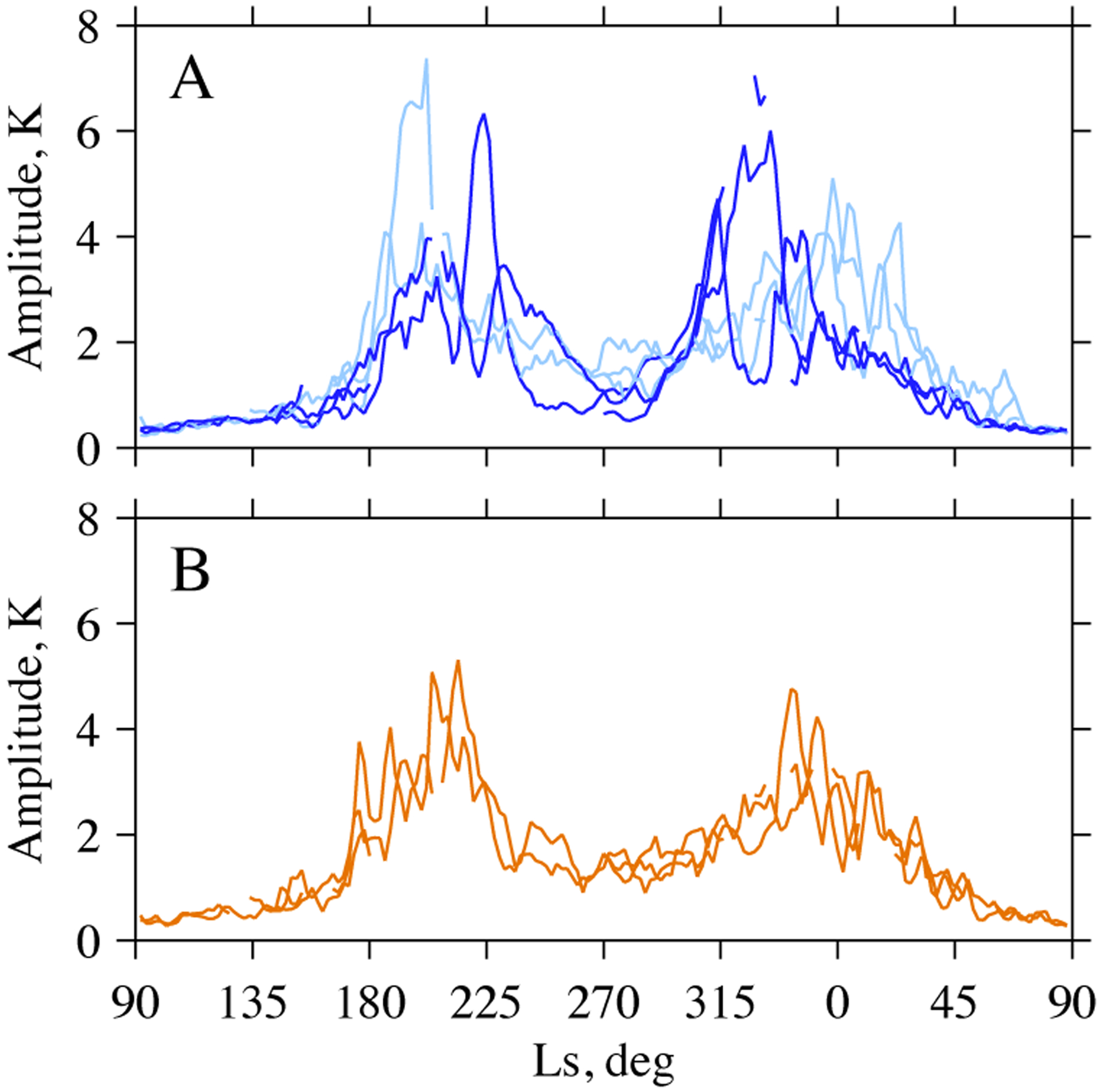
The meridional average of wave amplitude measured by TES at (orange) wave 1, (light blue) wave 2, and (dark blue) wave 3. For clarity, separate panels are used for (A) waves 2 and 3, and (B) wave 1. Observations affected by the PEDS that occurred in autumn of MY25 have been excluded from this figure. The results from each MY are shown individually in Fig. 13A. See Appendix B for a link to the data shown in this figure.

In Fig. 14, the average amplitude at each zonal wavenumber decreases to about 0.5 K in a period extending from late spring through early summer (L_s = 70–120°). This is the noise level of the MCS measurements, as indicated by an SNR that falls below the threshold of reliable wave detection (see Fig. 11). The amplitude at each zonal wavenumber exceeds the noise level throughout autumn and winter, though only by a small margin during the solstitial pause. In other words, a strong peak at one zonal wavenumber is typically accompanied by weaker activity at the other zonal wavenumbers. We return to this point at the end of this section.

Other aspects of the wave climatology can be identified by averaging the wave period with respect to latitude. For TES, the period is averaged within the same fixed latitude bands used in computing the average amplitude. For MCS, the average is limited to latitudes north of the curving boundaries in Fig. 12A–12C, which separate valid solutions for the wave period from low-latitude noise. Two other restrictions are applied in order to eliminate the least reliable results. First, latitude bins where the MCS SNR is less than 0.35 or the TES amplitude is less than 1.7 K are excluded from the average. Second, the average is discarded if fewer than four valid samples are available for a given value of L_s or if the samples are widely dispersed (specifically, if the standard deviation exceeds 20% of the average). The results appear in Fig. 16.

Figure 16:

The meridional average of wave period measured by (A) TES and (B) MCS at (orange) wave 1, (light blue) wave 2, and (dark blue) wave 3. Different symbols are used to distinguish the strongest mode in each bin of L_s (large circles) from the weaker modes (small triangles). This figure shows results from the same time periods covered by Figs. 14 and 15. TES results affected by the PEDS in autumn of MY25 have been excluded. See Appendix B for a link to the data shown in this figure.

There is no significant difference between the TES and MCS measurements in Fig. 16. With the addition of 5 MYs of MCS observations, the climatology of wave period is now well defined. The period varies with season at all zonal wavenumbers in a pattern that is roughly symmetric about the winter solstice. Between early autumn and late winter (L_s = 210–345°), the strongest modes (denoted by large circles) have typical periods of 6–8 sols at wave 1, 3–4 sols at wave 2, and 2–3 sols at wave 3. This activity corresponds to the primary peaks of the histograms in Fig. 10A–10C and 10E–10G. The wave period is longer before L_s = 210° and after L_s = 345°. For example, the wave-2 period increases steadily from about 3 sols at L_s = 345° to more than 10 sols at L_s = 45°. These patterns of behavior repeat closely from year to year.

The bin size of 14 sols places an upper limit on the period of the waves that can be detected reliably by our wave-search algorithm (Section 4). As the wave periods in Fig. 16 rarely reach this limit, our main conclusions are not affected by the choice of bin size. Overall, a bin size of 14 sols represents a reasonable compromise: it is longer than the period of most baroclinic waves and short enough to resolve most of the baroclinic wave transitions (Fig. 13).

The measurements in Fig. 16 illustrate another notable aspect of wave behavior. For both TES and MCS, the strong wave-3 mode at L_s = 210–250° and 290–340° is accompanied by wave-1 and wave-2 modes that are weaker in amplitude but have the same period (typically 2.2–2.4 sols). This superposition of modes describes a wave-3 baroclinic wave whose amplitude varies with longitude, as first identified through analysis of TES data by Banfield et al. (2004) and later studied in more detail through analysis of RO measurements of geopotential height (Hinson and Wang, 2010). All wave-3 modes exhibit this behavior (Hinson et al., 2012). A similar phenomenon occurs in both early autumn (L_s = 180–210°) and early spring (L_s = 0–30°), when a strong wave-2 mode is accompanied by a weaker wave-3 mode, both with the same period (typically 2.5–3.0 sols).

The observed variation of wave amplitude with longitude is a consequence of zonal variations of topography. GCM simulations have shown that the wave-surface interaction creates “storm zones” of enhanced wave amplitude (Hollingsworth et al., 1996; Basu et al., 2006), which are also apparent in TES observations (Banfield et al., 2004). The details of this interaction are discussed by Mooring and Wilson (2015), who used teleconnection maps to track the motion of highs and lows of surface pressure in the TES reanalysis. They found that phase propagation near the surface tends to follow the topography, with eddies moving northward around obstacles such as Alba Mons and dipping southward into the topographic basins. The meridional motion of the eddies in turn modulates their relative vorticity. For these reasons, the wave amplitude will vary with longitude when observed at fixed latitude, as in the method of analysis used here.

6.3. Baroclinic waves and dust storms

In this section we examine the connections between baroclinic waves and dust storms, focusing on events that have a global impact on dust opacity and temperature, but excluding PEDS. Specifically, we are interested in the mid-autumn “A” storms and the mid-winter “C” storms in the nomenclature of Kass et al. (2016). Though much weaker than a PEDS, the A and C storms still produce significant changes in the global circulation, as reflected by a large increase in the zonal-mean temperature at 50 Pa (Kass et al., 2016). We describe them here in terms of their effect on dust opacity, using the dust climatology assembled by Montabone et al. (2015) from observations by several spacecraft (www-mars.lmd.jussieu.fr/mars/dust_climatology/index.html). This database comprises daily maps of dust column absorption at 9.3 microns; the maps used here are uniformly gridded and normalized to 610 Pa.

Fig. 17 compares the zonal-mean dust opacity with selected properties of the baroclinic waves in MY24, 26, and 29–33. (MY25 is omitted because of the PEDS in autumn and several data gaps in winter.) The opacity exceeds 0.4 over a broad range of latitudes during the strongest storms, which occurred in winter of MY26 and autumn of MY24, 29, and 32; in each case there is a rapid increase in opacity followed by a more gradual decay. Events that are similar in character though weaker in magnitude occurred in both autumn and winter of every MY shown here. Their timing and magnitude vary considerably from year to year. For example, the A storm arrived much earlier in MY31 than in MY29, and the dust storms were unusually weak in both autumn and winter of MY30. Each panel of Fig. 17 also shows contemporaneous measurements of wave-3 amplitude in two formats. First, contours of wave amplitude show the seasonal evolution of the wave and its location in latitude (as in Fig. 11). Second, each panel includes a line drawing of average amplitude (shown previously in Fig. 13). We focus on the wave-3 mode because most of the A and C storms begin when it is the strongest mode.

Figure 17:

(color) Maps of zonal-mean dust column absorption at 9.3 microns (Montabone et al., 2015) versus latitude (left ordinate) and L_s. Black contours show zonal-mean opacities at levels denoted by tick marks in the color bar, which applies to all seven panels. A contour map of wave-3 amplitude is superimposed (yellow), showing the seasonal evolution of the wave and its location in latitude; the contour spacing is 1 K for TES (top row) and 0.5 K for MCS (all other rows). Line drawings show the average amplitude (right ordinate) of the wave-3 mode (solid white line in all panels) and the wave-2 mode (dashed white line in MY31 only).

Fig. 17 implies that baroclinic waves and dust storms are linked in two important ways. The first interaction occurs as a dust storm begins. A prominent peak in wave-3 amplitude is aligned with the rapid growth in opacity at the start of the largest A storms (MY24, 29, and 32) and C storms (MY26, 31, and 33). This is consistent with previous results derived from MGS data (MY24–26), which showed that baroclinic waves help initiate the A and C storms by launching flushing dust storms that travel from high northern latitudes into the tropics (Wang et al., 2005; Wang, 2007; Hinson et al., 2012; Wang et al., 2013; Wang, 2018; Battalio and Wang, 2020). The 5 MYs of MCS observations in Fig. 17 corroborate the MGS results and suggest that the wave-3 mode is responsible for a large part of the year-to-year variability in the timing of both A and C storms.

In some years the A storm begins when wave 2 is the strongest mode, as noted previously by Wang (2007). For example, Fig. 17 shows that the start of the A storm in MY31 is aligned with a strong peak in the amplitude of the wave-2 mode. The same is true in MY26 and 33 (not shown), which suggests that the wave-2 mode helps initiate some A storms, specifically the ones that begin relatively early in autumn. It’s not clear why this happens in some years but not others. This variability cannot be attributed entirely to the strength of the early-autumn wave-2 mode — its amplitude was larger in MY32 than in any other year observed by MCS (Fig. 13) yet it failed to initiate an early A storm.

In the second type of interaction, the growth of the dust storm is accompanied by a rapid decrease in the wave-3 amplitude, so that the amplitude is anti-correlated with peaks in zonal-mean opacity. For example, the strong wave-3 modes that helped initiate large A storms in MY24, 29, and 32 had largely vanished by the time the zonal-mean opacity reached its maximum value. Dust-storm suppression of the baroclinic waves is especially striking in winter of MY26, 30, and 32, when the wave-3 mode has two or more peaks in amplitude separated by intervening periods of enhanced zonal-mean dust opacity. Taken together, the 7 MYs of observations in Fig. 17 provide compelling evidence for suppression of the wave-3 mode by A and C dust storms. In some MYs the solstitial pause begins in response to this process.

Both types of interaction were identified previously by Battalio and Wang (2020) through analysis of MGS data from MY24 and 26. With the addition of 5 MYs of new observations, Fig. 17 provides much stronger evidence for the close linkage between baroclinic waves and dust storms, while demonstrating its importance to the current climate.

In the preceding discussion, we assumed that the A and C storms do not reduce the ability of MCS or TES to accurately monitor the baroclinic waves. This assumption appears to be valid for the following reason. The A and C storms have a relatively small impact on dust opacity at the latitude of the baroclinic waves, about 40–70°N (Fig. 17). It seems unlikely that the storm-induced change in dust opacity is sufficient to conceal the waves throughout this latitude range, particularly at latitudes north of 55°N.

7. Conclusions

The characteristics of the baroclinic waves observed by MCS and TES are largely the same, including the statistics of wave period (Fig. 10), the properties of individual wave modes (Figs. 11 and 12), and the symmetry of wave activity about the solstitial pause (Figs. 14 and 15). The similarity extends from detailed aspects of wave behavior, such as the zonal modulation of the wave-3 mode, to the wave climatology (Figs. 14–16). These comparisons illustrate the quality of the MCS results and the capacity of the B1 channel for remote sensing of low-altitude baroclinic waves.

Several well-defined patterns of behavior are apparent in the extensive record of baroclinic wave activity derived in this paper. For example, the measurements show that baroclinic wave transitions are an intrinsic property of the weather on Mars (Fig. 13), as implied previously by Viking Lander pressure measurements (Collins et al., 1996) and RO measurements of geopotential height (Hinson, 2006; Hinson and Wang, 2010). There are significant year-to-year variations in both the amplitude of individual wave modes and the timing of the mode transitions, but a composite of observations from all MYs reveals limits on the range of variability that define the wave climatology (Figs. 14–16). One notable example is the order of appearance of the three principal wave modes. The zonal wavenumber of the strongest mode shifts from wave 2 near both equinoxes to wave 3 in mid-autumn and mid-winter, immediately before and after the solstitial pause. In addition, the meridional averages of wave amplitude and period exhibit mirror-image symmetry about the winter solstice.

Fig. 17 places the wave measurements into context with the Martian dust cycle, yielding two important conclusions. First, the wave-3 mode is a common precursor to both mid-autumn A storms and mid-winter C storms, which reflects its importance in initiating those events. Second, the wave-3 mode decays rapidly in response to the subsequent increase in zonal-mean dust opacity as the A and C storms evolve. This is probably a consequence of dust-induced changes in the global circulation, which modify the structure of the baroclinic zone in a way that reduces instability (Mulholland et al., 2016; Battalio et al., 2016; Lee et al., 2018).

The results reported here provide a foundation for future work in several areas. For example, the performance of a free-running GCM can be evaluated by comparing the wave climatology in Figs. 14–16 with analogous results derived from a multi-year numerical simulation. The observed dust-storm suppression of the wave-3 mode (Fig. 17) also provides a valuable benchmark. These comparisons could lead to improvements in modeling the radiative effects of water-ice clouds, which have a large impact on the properties of the simulated waves (e.g., Haberle et al., 2019), and to more accurate predictions for aspects of wave behavior that cannot be measured directly.

Flushing dust storms are not uniformly distributed among the three topographic basins of the northern hemisphere, and both their timing and intensity vary considerably from year to year. A detailed investigation of this aspect of the dust cycle is now possible by comparing the phasing in longitude of an individual wave mode with contemporaneous observations of dust storms by the MGS MOC and the MRO MARCI (Wang and Richardson, 2015; Battalio and Wang, 2020). One objective is to determine the degree to which the timing, location, and year-to-year variability of the dust storms are controlled by the characteristics of the baroclinic waves and the transitions among modes with different zonal wavenumbers.

Finally, we plan to use a similar approach to characterize baroclinic waves in the southern hemisphere, where the waves are known to be weaker than those in the north (Banfield et al., 2004; Lewis et al., 2016; Barnes et al., 2017). The main objective is to derive a wave climatology analogous to the one in Figs. 14–16.

Highlights.

• The weather at low altitudes in the northern hemisphere of Mars is investigated

• Properties of baroclinic waves are derived from IR observations by two spacecraft

• The waves exhibit periodic transitions among modes with different zonal wavenumbers

• A well-defined wave climatology emerges from results spanning 8 Mars years

• Baroclinic waves initiate dust storms, which in turn suppress the baroclinic waves

A. Analysis of temperatures retrieved by MCS

We downloaded MCS Derived Data Records (version 5) from the NASA PDS and extracted samples of temperature at 610 Pa (T₆₁₀). Only 2D retrievals are used here. Baroclinic waves were identified and characterized by applying the method of analysis described in Section 4. The results, which appear in Figs. 18 and 19, are from 1 MY of observations beginning at L_s = 90° of MY30.

Figure 18:

(A)–(C) Wave amplitude derived from measurements of T₆₁₀ spanning 1 MY (L_s = 90° of MY30 through L_s =90° of MY31). (D)–(F) Analogous results derived from contemporaneous measurements of brightness temperature in the MCS B1 channel. See caption to Fig. 11 for further explanation.

Figure 19:

(A)–(C) Wave period derived from measurements of T₆₁₀ spanning 1 MY (L_s =90° of MY30 through L_s =90° of MY31). (D)–(F) Analogous results derived from contemporaneous measurements of brightness temperature in the MCS B1 channel. Arrows identify specific modes discussed in the text. See caption to Fig. 12 for further explanation.

Panels A–C of Fig. 18 show the wave amplitude derived from T₆₁₀ at zonal wavenumber 1–3. MCS profiles rarely reach 610 Pa at latitudes experiencing polar night, which makes that region inaccessible; the gap in coverage extends well into the surrounding baroclinic zone. Panels D–F of Fig. 18 show the corresponding results derived from observations in the MCS B1 channel, as discussed previously in Section 5.4. The strongest wave modes detected by T₆₁₀ are also apparent in the B1 channel. These include a prominent wave-2 mode in early autumn and a double-peaked wave-3 mode in mid-winter, which is resolved more clearly by the B1 channel. A different color bar is used for each type of observation; the amplitude in 32-micron brightness temperature is roughly half as large as the amplitude in physical temperature (T₆₁₀).

The consistency between the two sets of observations is demonstrated more clearly by a comparison of wave period, as shown in Fig. 19. There are many instances of matching period, such as a 7-sol wave-1 mode in mid-autumn, a 4-sol wave-2 mode in early spring, and a 2.3-sol wave-3 mode in mid-winter; these three modes are identified by arrows in Fig. 19.

In summary, both the quality and the spatial coverage of the T₆₁₀ results are limited by the scarcity of MCS profiles at this pressure level. Nonetheless, the results in Figs. 18 and 19 confirm that the 32-micron brightness temperature is sensitive to wave activity near the 610-Pa pressure level.

B. Supplementary data

Figs. 13–16 show meridional averages of amplitude and period. The data in those figures can be found in the online version of this paper at INSERT DOI AND LINK. There are two files, one for MCS and one for TES, both in the same format. Each file contains seven columns of ASCII text. Column 1 is L_s (degrees) measured cumulatively from the start of MY24. Column 2 is the average amplitude (K) of the wave-1 mode. Column 3 is the average period (sols) of the wave-1 mode. Columns 4 and 5 are the average amplitude and period, respectively, of the wave-2 mode. Columns 6 and 7 are the average amplitude and period, respectively, of the wave-3 mode. The amplitude is set to zero in data gaps. The period is set to zero not only in data gaps but also in cases where the average period is not well determined, as explained in Section 6.2.

References

- Banfield D, Conrath BJ, Gierasch PJ, Wilson RJ, Smith MD, 2004. Traveling waves in the martian atmosphere from MGS TES nadir data. Icarus 170, 365–403. doi: 10.1016/j.icarus.2004.03.015. [DOI] [Google Scholar]
- Banfield D, Spiga A, Forget F, Newman CE, Garcia RF, Kass DM, Kleinboehl A, 2020a. Baroclinic Waves, Infrasound, and Pressure Bursts on Mars from InSight, in: 51st Lunar and Planetary Science Conference, p. 2438. [Google Scholar]
- Banfield D, Spiga A, Newman C, et al. , 2020b. The atmosphere of Mars as observed by InSight. Nature Geoscience 13, 190–198. doi: 10.1038/s41561-020-0534-0. [DOI] [Google Scholar]
- Barnes JR, 1980. Time spectral analysis of midlatitude disturbances in the Martian atmosphere. Journal of the Atmospheric Sciences 37, 2002–2015. doi: 10.1175/1520-0469(1980)037. [DOI] [Google Scholar]
- Barnes JR, 1981. Midlatitude disturbances in the Martian atmosphere - A second Mars year. Journal of the Atmospheric Sciences 38, 225–234. doi: 10.1175/1520-0469(1981)038. [DOI] [Google Scholar]
- Barnes JR, Haberle RM, Wilson RJ, Lewis SR, Murphy JR, Read PL, 2017. The Global Circulation. In: Haberle RM, Clancy RT, Forget F, Smith MD, Zurek RW (Eds.), The Atmosphere and Climate of Mars. Cambridge University Press. pp. 229–294. doi: 10.1017/9781139060172.009. [DOI] [Google Scholar]
- Basu S, Wilson J, Richardson M, Ingersoll A, 2006. Simulation of spontaneous and variable global dust storms with the GFDL Mars GCM. Journal of Geophysical Research (Planets) 111, E09004. doi: 10.1029/2005JE002660. [DOI] [Google Scholar]
- Battalio M, Szunyogh I, Lemmon M, 2016. Energetics of the martian atmosphere using the Mars Analysis Correction Data Assimilation (MACDA) dataset. Icarus 276, 1–20. doi: 10.1016/j.icarus.2016.04.028. [DOI] [Google Scholar]
- Battalio M, Wang H, 2020. Eddy evolution during large dust storms. Icarus 338, 113507. doi: 10.1016/j.icarus.2019.113507. [DOI] [Google Scholar]
- Calvin WM, James PB, Cantor BA, Dixon EM, 2015. Interannual and seasonal changes in the north polar ice deposits of Mars: Observations from MY 29–31 using MARCI. Icarus 251, 181–190. doi: 10.1016/j.icarus.2014.08.026. [DOI] [Google Scholar]
- Clancy RT, Sandor BJ, Wolff MJ, Christensen PR, Smith MD, Pearl JC, Conrath BJ, Wilson RJ, 2000. An intercomparison of ground-based millimeter, MGS TES, and Viking atmospheric temperature measurements: Seasonal and interannual variability of temperatures and dust loading in the global Mars atmosphere. Journal of Geophysical Research (Planets) 105(E4), 9553–9572. doi: 10.1029/1999JE001089. [DOI] [Google Scholar]
- Collins M, Lewis SR, Read PL, Hourdin F, 1996. Baroclinic Wave Transitions in the Martian Atmosphere. Icarus 120, 344–357. doi: 10.1006/icar.1996.0055. [DOI] [Google Scholar]
- Conrath BJ, Pearl JC, Smith MD, Maguire WC, Christensen PR, Dason S, Kaelberer MS, 2000. Mars Global Surveyor Thermal Emission Spectrometer (TES) observations: Atmospheric temperatures during aerobraking and science phasing. Journal of Geophysical Research (Planets) 105, 9509–9519. doi: 10.1029/1999JE001095. [DOI] [Google Scholar]
- Greybush SJ, Gillespie HE, Wilson RJ, 2019. Transient eddies in the TES/MCS Ensemble Mars Atmosphere Reanalysis System (EMARS). Icarus 317, 158–181. doi: 10.1016/j.icarus.2018.07.001. [DOI] [PMC free article] [PubMed] [Google Scholar]
- Haberle RM, Juárez M.d.l.T., Kahre MA, Kass DM, Barnes JR, Hollingsworth JL, Harri AM, Kahanpää H, 2018. Detection of Northern Hemisphere transient eddies at Gale Crater Mars. Icarus 307, 150–160. doi: 10.1016/j.icarus.2018.02.013. [DOI] [Google Scholar]
- Haberle RM, Kahre MA, Hollingsworth JL, Montmessin F, Wilson RJ, Urata RA, Brecht AS, Wolff MJ, Kling AM, Schaeffer JR, 2019. Documentation of the NASA/Ames Legacy Mars Global Climate Model: Simulations of the present seasonal water cycle. Icarus 333, 130–164. doi: 10.1016/j.icarus.2019.03.026. [DOI] [Google Scholar]
- Hinson DP, 2006. Radio occultation measurements of transient eddies in the northern hemisphere of Mars. Journal of Geophysical Research (Planets) 111, E05002. doi: 10.1029/2005JE002612. [DOI] [Google Scholar]
- Hinson DP, Wang H, 2010. Further observations of regional dust storms and baroclinic eddies in the northern hemisphere of Mars. Icarus 206, 290–305. doi: 10.1016/j.icarus.2009.08.019. [DOI] [Google Scholar]
- Hinson DP, Wang H, Smith MD, 2012. A multi-year survey of dynamics near the surface in the northern hemisphere of Mars: Short-period baroclinic waves and dust storms. Icarus 219, 307–320. doi: 10.1016/j.icarus.2012.03.001. [DOI] [Google Scholar]
- Hinson DP, Wilson RJ, 2002. Transient eddies in the southern hemisphere of Mars. Geophysical Research Letters 29(7), 1154. doi: 10.1029/2001GL014103. [DOI] [Google Scholar]
- Hollingsworth JL, Haberle RM, Barnes JR, Bridger AFC, Pollack JB, Lee H, Schaeffer J, 1996. Orographic control of storm zones on Mars. Nature 380, 413–416. doi: 10.1038/380413a0. [DOI] [Google Scholar]
- Kass DM, Kleinböhl A, McCleese DJ, Schofield JT, Smith MD, 2016. Interannual similarity in the Martian atmosphere during the dust storm season. Geophysical Research Letters 43, 6111–6118. doi: 10.1002/2016GL068978. [DOI] [Google Scholar]
- Kleinböhl A, Schofield JT, Kass DM, Abdou WA, Backus CR, Sen B, Shirley JH, Lawson WG, Richardson MI, Taylor FW, Teanby NA, McCleese DJ, 2009. Mars Climate Sounder limb profile retrieval of atmospheric temperature, pressure, and dust and water ice opacity. Journal of Geophysical Research (Planets) 114(E10), E10006. doi: 10.1029/2009JE003358. [DOI] [Google Scholar]
- Lee C, Richardson MI, Newman CE, Mischna MA, 2018. The sensitivity of solsticial pauses to atmospheric ice and dust in the MarsWRF General Circulation Model. Icarus 311, 23–34. doi: 10.1016/j.icarus.2018.03.019. [DOI] [Google Scholar]
- Leovy C, Mintz Y, 1969. Numerical Simulation of the Atmospheric Circulation and Climate of Mars. Journal of the Atmospheric Sciences 26, 1167–1190. doi:. [DOI] [Google Scholar]
- Leovy CB, Tillman JE, Guest WR, Barnes JR, 1985. Interannual variability of martian weather. In: Hunt GE (Ed.), Recent Advances in Planetary Meteorology. Cambridge University Press, New York. pp. 69–84. [Google Scholar]
- Lewis SR, Mulholland DP, Read PL, Montabone L, Wilson RJ, Smith MD, 2016. The solsticial pause on Mars: 1. A planetary wave reanalysis. Icarus 264, 456–464. doi: 10.1016/j.icarus.2015.08.039. [DOI] [Google Scholar]
- McCleese DJ, Schofield JT, Taylor FW, Calcutt SB, Foote MC, Kass DM, Leovy CB, Paige DA, Read PL, Zurek RW, 2007. Mars Climate Sounder: An investigation of thermal and water vapor structure, dust and condensate distributions in the atmosphere, and energy balance of the polar regions. Journal of Geophysical Research (Planets) 112(E05), E05S06. doi: 10.1029/2006JE002790. [DOI] [Google Scholar]
- Montabone L, Forget F, Millour E, Wilson RJ, Lewis SR, Cantor B, Kass D, Kleinböhl A, Lemmon MT, Smith MD, Wolff MJ, 2015. Eight-year climatology of dust optical depth on Mars. Icarus 251, 65–95. doi: 10.1016/j.icarus.2014.12.034. [DOI] [Google Scholar]
- Mooring TA, Wilson RJ, 2015. Transient eddies in the MACDA Mars reanalysis. Journal of Geophysical Research (Planets) 120, 1671–1696. doi: 10.1002/2015JE004824. [DOI] [Google Scholar]
- Mulholland DP, Lewis SR, Read PL, Madeleine JB, Forget F, 2016. The solsticial pause on Mars: 2 modelling and investigation of causes. Icarus 264, 465–477. doi: 10.1016/j.icarus.2015.08.038. [DOI] [Google Scholar]
- Pankine AA, 2015. The nature of the systematic radiometric error in the MGS TES spectra. Planetary and Space Science 109, 64–75. doi: 10.1016/j.pss.2015.01.022. [DOI] [Google Scholar]
- Ryan JA, Henry RM, Hess SL, Leovy CB, Tillman JE, Walcek C, 1978. Mars meteorology - Three seasons at the surface. Geophysical Research Letters 5, 715–718. doi: 10.1029/GL005i008p00715. [DOI] [Google Scholar]
- Ryan JA, Sharman RD, 1981. Two major dust storms, one Mars year apart - Comparison from Viking data. Journal of Geophysical Research 86, 3247–3254. doi: 10.1029/JC086iC04p03247. [DOI] [Google Scholar]
- Salby ML, 1982. Sampling theory for asynoptic satellite observations. Part I: Space-time spectra, resolution, and aliasing. Journal of the Atmospheric Sciences 39, 2577–2600. [Google Scholar]
- Smith MD, 2004. Interannual variability in TES atmospheric observations of Mars during 1999–2003. Icarus 167, 148–165. doi: 10.1016/j.icarus.2003.09.010. [DOI] [Google Scholar]
- Smith MD, Pearl JC, Conrath BJ, Christensen PR, 2001. Thermal Emission Spectrometer results: Mars atmospheric thermal structure and aerosol distribution. Journal of Geophysical Research 106, 23929–23945. doi: 10.1029/2000JE001321. [DOI] [Google Scholar]
- Wang H, 2007. Dust storms originating in the northern hemisphere during the third mapping year of Mars Global Surveyor. Icarus 189, 325–343. doi: 10.1016/j.icarus.2007.01.014. [DOI] [Google Scholar]
- Wang H, 2018. Cross-Equatorial Flushing Dust Storms and Northern Hemisphere Transient Eddies: An Analysis for Mars Year 24. Journal of Geophysical Research (Planets) 123, 1732–1745. doi: 10.1029/2018JE005623. [DOI] [PMC free article] [PubMed] [Google Scholar]
- Wang H, Richardson MI, 2015. The origin, evolution, and trajectory of large dust storms on Mars during Mars years 24–30 (1999–2011). Icarus 251, 112–127. doi: 10.1016/j.icarus.2013.10.033. [DOI] [Google Scholar]
- Wang H, Richardson MI, Toigo AD, Newman CE, 2013. Zonal wavenumber three traveling waves in the northern hemisphere of Mars simulated with a general circulation model. Icarus 223, 654–676. doi: 10.1016/j.icarus.2013.01.004. [DOI] [Google Scholar]
- Wang H, Zurek RW, Richardson MI, 2005. Relationship between frontal dust storms and transient eddy activity in the northern hemisphere of Mars as observed by Mars Global Surveyor. Journal of Geophysical Research (Planets) 110(E9), E07005. doi: 10.1029/2005JE002423. [DOI] [Google Scholar]
- Wilson RJ, Banfield D, Conrath BJ, Smith MD, 2002. Traveling waves in the Northern Hemisphere of Mars. Geophysical Research Letters 29(14), 1684. doi: 10.1029/2002GL014866. [DOI] [Google Scholar]
- Zurek RW, Barnes JR, Haberle RM, Pollack JB, Tillman JE, Leovy CB, 1992. Dynamics of the atmosphere of Mars. In: Kieffer HH, Jakosky BM, Snyder CW, Matthews MS (Eds.), Mars. Univ. of Arizona Press, Tucson. pp. 835–933. [Google Scholar]
Associated Data
This section collects any data citations, data availability statements, or supplementary materials included in this article.