Abstract
Purpose:
The developments of PET/CT and PET/MR scanners provide opportunities for improving PET image quality by using anatomical information. In this paper, we propose a novel co-learning 3D convolutional neural network (CNN) to extract modality-specific features from PET/CT image pairs and integrate complementary features into an iterative reconstruction framework to improve PET image reconstruction.
Methods:
We used a pre-trained deep neural network to represent PET images. The network was trained using low-count PET and CT image pairs as inputs and high-count PET images as labels. This network was then incorporated into a constrained maximum likelihood framework to regularize PET image reconstruction. Two different network structures were investigated for the integration of anatomical information from CT images. One was a multi-channel CNN, which treated PET and CT volumes as separate channels of the input. The other one was multi-branch CNN, which implemented separate encoders for PET and CT images to extract latent features and fed the combined latent features into a decoder. Using computer-based Monte Carlo simulations and two real patient datasets, the proposed method has been compared with existing methods, including the maximum likelihood expectation maximization (MLEM) reconstruction, a kernel-based reconstruction and a CNN-based deep penalty method with and without anatomical guidance.
Results:
Reconstructed images showed that the proposed constrained ML reconstruction approach produced higher quality images than the competing methods. The tumors in the lung region have higher contrast in the proposed constrained ML reconstruction than in the CNN-based deep penalty reconstruction. The image quality was further improved by incorporating the anatomical information. Moreover, the liver standard deviation was lower in the proposed approach than all the competing methods at a matched lesion contrast.
Conclusions:
The supervised co-learning strategy can improve the performance of constrained maximum likelihood reconstruction. Compared with existing techniques, the proposed method produced a better lesion contrast vs. background standard deviation trade-off curve, which can potentially improve lesion detection.
I. Introduction
Positron emission tomography (PET) is a widely used clinical imaging modality for cancer diagnosis, staging and treatment response assessment1. Due to the potential radiation risk associated with the radioactive tracers, the injected activity in each PET scan is limited. As a result, PET data have low count statistics. Recent advances in PET instrumentation have focused on improving the photon detection sensitivity by measuring time-of-flight (TOF) information2 and extending the axial field of view (FOV)3.
Noise in PET data can be further amplified in the image reconstruction process, resulting in noisy reconstructed images. In order to improve image reconstruction performance, prior information has been introduced to regularize the reconstruction. Instead of maximizing the likelihood function directly, the algorithm maximizes the posterior distribution. A common prior model is Tikhonov regularization, which assumes the images are smooth and continuous and consequently blurs sharp edges during reconstruction. To address this issue, other penalty terms, such as total variation (TV)4 and patched based penalties5 have been proposed to reduce the extent of blurring. However, these techniques still have limited ability to distinguish an edge from noise.
Since the spatial distribution of a radioactive tracer should be associated with anatomical structures, anatomical information from a co-registered CT or MRI can be applied to build an appropriate prior model. One challenge in anatomy-guided PET reconstruction is the existence of mismatches between different modalities that measure different morphological or functional information. A variety of methods have been developed to solve the mismatch issues, such as segmentation based A-MAP6,7, Bowsher’s similarity method8, the joint entropy prior9, and level-set prior10. Hutchcroft et al11 applied the kernel method12 to anatomy-guided PET reconstruction using an anatomical image derived kernel matrix. This method has been extended to incorporate both PET and MRI derived kernel matrices based on the structural similarity metric13. Other interesting methods and comparisons between them can be found in14,15,16. All of the above methods try to find an appropriate similarity measure to weigh PET and MRI features differently. Users can also manually adjust hyper-parameters, such as a predefined neighborhood size or the tolerance for relative differences, to emphasize modality-specific features. But the complexity of these adjustments introduces another new problem: lack of reproducibility.
Deep learning17, due to its unprecedented success in tasks such as image classification, segmentation, inpainting, and denoising, has found applications in medical image reconstruction. The convolutional neural network (CNN) is capable of implicitly fusing anatomical and functional features from multi-modality image data with proper training. Studies18,19 have shown that co-learning features from PET-CT significantly increase tumor segmentation accuracy, compared with the use of a single modality. For image denoising, Lei et al.20 proposed a deep learning architecture to estimate the high-quality PET images from the combination of low-count PET and T1-weighted MRI. Liu and Qi21 trained three modified U-Nets to improve the PET signal-to-noise ratio (SNR) with PET/MRI images. Similarly, Costa-Luis and Reader22 used a low-complexity CNN as an MR-aided image processing step to reduce noise and reconstruction artefacts. Subsequently, Cui et al.23 presented a deep image prior24 denoising method to leverage CT/MR information without using a high-count PET label. The cycle consistent generative adversarial network (GAN) was also utilized in PET denoising to predict diagnostic quality PET images with25,26 and without anatomical aids27,28. The cycle GAN algorithm not only learns a transformation to synthesize high-count PET images using low-count images but also learns an inverse transformation to ensure that pseudo low-count PET images generated from synthetic high-count PET are close to the true low-count PET images. Despite the fact that these approaches improve the model’s prediction, pathological abnormalities and patient-to-patient variations may reduce the robustness of these end-to-end denoising methods. Some instability phenomena have been reported in29.
In order to safely use deep learning methods in medical imaging, data consistency needs to be taken into account. Besides the post-processing reconstructed images, deep learning has emerged as a new tool in image reconstruction30,31,32. The various types of methods were introduced in a very short period of time, such as direct inversion33,34, image regularization35, and unrolling approaches36. The approach of using a deep image prior24 has also been applied to anatomically aided PET reconstruction37.
Our aim in this paper is to improve the fusion of the complementary information in PET/CT or PET/MRI images for anatomy-aided reconstruction. In particular, we focus on the network-constrained image reconstruction method38,39, where a denoising CNN, trained by high-quality images, is used to represent feasible PET images in a constrained maximum likelihood reconstruction framework. The low-count PET and CT images are used as inputs to train a 3D denoising CNN with high-count PET images as labels. The unknown PET image during a reconstruction is represented as the output of a pre-trained CNN in a constrained maximum likelihood framework. We investigated two different co-learning strategies. One is a multi-channel input CNN20,40, which treats PET and CT volumes as two channels of the input. The other is a multi-branch CNN19,41, which implements separate encoders for PET and CT images to extract features and concatenates the latent features before the decoder. By using computer-based Monte Carlo simulations and two real patient datasets, we compared the proposed method with existing methods, including EM reconstruction with Gaussian filtering, kernel-based reconstruction, and the CNN-based deep penalty method with and without anatomical guidance.
II. Methods and materials
II.A. Theoretical framework
The data model used in this work considers the measured PET data y as a collection of independent Poisson random variables. For a typical PET system with M number of lines of response (LOR) and N number of image voxels, the expectation of measured counts, , can be expressed by
| (1) |
where is the unknown radioactive tracer distribution, and is the detection probability matrix. The (i, j)th element of P, pi,j, represents the probability that an emission originated in the jth voxel is detected by the ith LOR. and are the expected number of scattered and randoms coincidences, respectively. The Poisson log-likelihood function is given by
| (2) |
Then the unknown image x can be estimated by the maximum likelihood estimator:
| (3) |
To improve the image quality and reduce noise, we adopt a constrained maximum likelihood estimation framework. Basically, the unknown PET image x is represented by the output of a pre-trained CNN with multi-modality images, such as PET/CT or PET/MRI, as the input:
| (4) |
where denotes the pre-trained denoising neural network and α denotes the inputs to the network. Compared with previous work38,39, the network inputs in this study not only include a noisy PET image (αPET) but also a co-registered anatomical image (αCT or αMRI). Here we will focus on using CT images as an application example. Then the PET image is estimated by solving the following constrained maximum likelihood estimation problem:
| (5) |
The network is trained off-line by using ML-EM reconstructions of high-count PET data as labels. When we only use PET images as the input to the network, the formulation of equation (5) simplifies to the previous method38. We apply the augmented Lagrangian method to the constrained optimization problem in (5) and obtain
| (6) |
where represents the vector of Lagrange multipliers and ρ > 0 is a hyperparameter, which affects the convergence speed but does not change the final solution at convergence. When the algorithm is stopped before convergence, a larger ρ generally results in a smoother image. In this study, we empirically chose the value of ρ based on the reconstruction of the validation data. Equation (6) can be maximized by the alternating direction method of multipliers (ADMM) algorithm42 in three steps:
| (7) |
| (8) |
| (9) |
We solve equation (7) by using the optimized transfer method5:
| (10) |
where and is obtained by the MLEM update:
| (11) |
The subproblem (8) can be solved using a gradient ascent algorithm:
| (12) |
We use ‘tf.GradientTape’ API of TensorFlow for automatic differentiation. As the intensity of network input is normalized, once a proper step size S is found, it can be used for different datasets. In this work, we use S = 0.01 for all three different datasets. It should be noted that, there is no update on the anatomical input, i.e., αCT remains the same during iterations.
II.B. Network architecture
In this work, we investigated two co-learning strategies and compared the results with those from the single-modality (PET only) CNN. Fig. 1 shows the structure of the three networks. For combining functional (PET) image and structural (CT) images, we start with a multi-channel input CNN modified from the U-net43 as shown in Fig.1 (b), which treats PET/CT images as two separate input channels. Except the first convolutional layer, multi-channel input CNN has the same architecture as the PET-only input CNN shown in Fig.1 (a). Specifically, the first convolutional layer contains 16 filters of support 3×3×3×c, where c is the number of input channels (with c=1 for PET-only CNN and c=2 for multi-channel input CNN), and 3×3×3 denotes the spatial size of the filter. The second co-learning architecture is a multi-branch CNN shown in Fig.1 (c), which implements separate encoders for PET and CT images. The modality-specific features generated by two encoders are concatenated channel-wise. In this work, we also include a self-attention module to learn the optimal weights of features in the latent space44,45. Essentially, the self-attention module reweighs features in a certain layer of the network according to inter-dependencies of different features. Similar to a non-local means filter, the self-attention module tries to capture long-range spatial dependencies. In our previous work46, we demonstrated that the U-net with a self-attention module outperforms the U-net without a self-attention module. For multi-branch input network, the self-attention module enables to weigh modality-specific features at different locations, which is expected to efficiently fuse features from the two encoders. All three networks have the same decoder for synthesizing high-count PET images.
Figure 1:
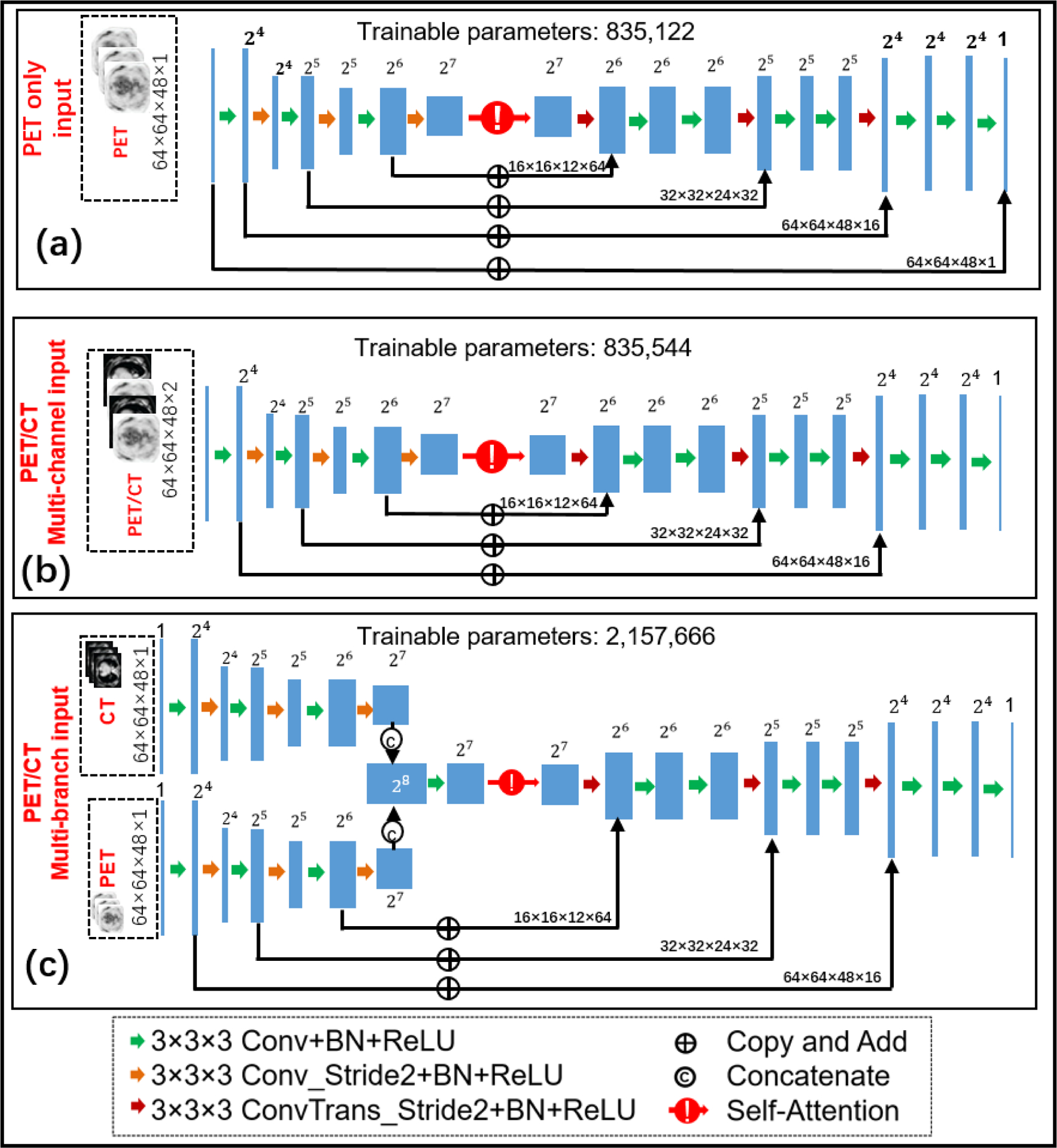
The architecture of three 3D deep neural networks with (a) PET input only, (b) PET/CT multi-channel input and (c) PET/CT multi-branch input, respectively. The input to each modality-specific encoder is a 3D patch of the corresponding modality.
We train the networks using the adaptive moment estimation (Adam) optimizer47 with following loss function
| (13) |
where αCT, αPET and x denote co-registered CT images, low and high count PET images, respectively. The training was implemented using the open-source library Keras 2.2.5 with Tensorflow backbone and trained on an NVIDIA GTX 1080 Ti GPU. Considering limited graphics processing unit (GPU) memory, 3D patches (64×64×48) from input images were extracted for training by sliding a window on each image with a stride of 32. We empirically set the mini-batch size to 8, the number of epochs to 1000, and the decayed learning rate schedule as follows: initial value was set to 0.004 and decay of rate 0.5 every 400 epochs. The L2 losses of the training and validation datasets for each epoch were saved and are shown in Fig. 2.
Figure 2:
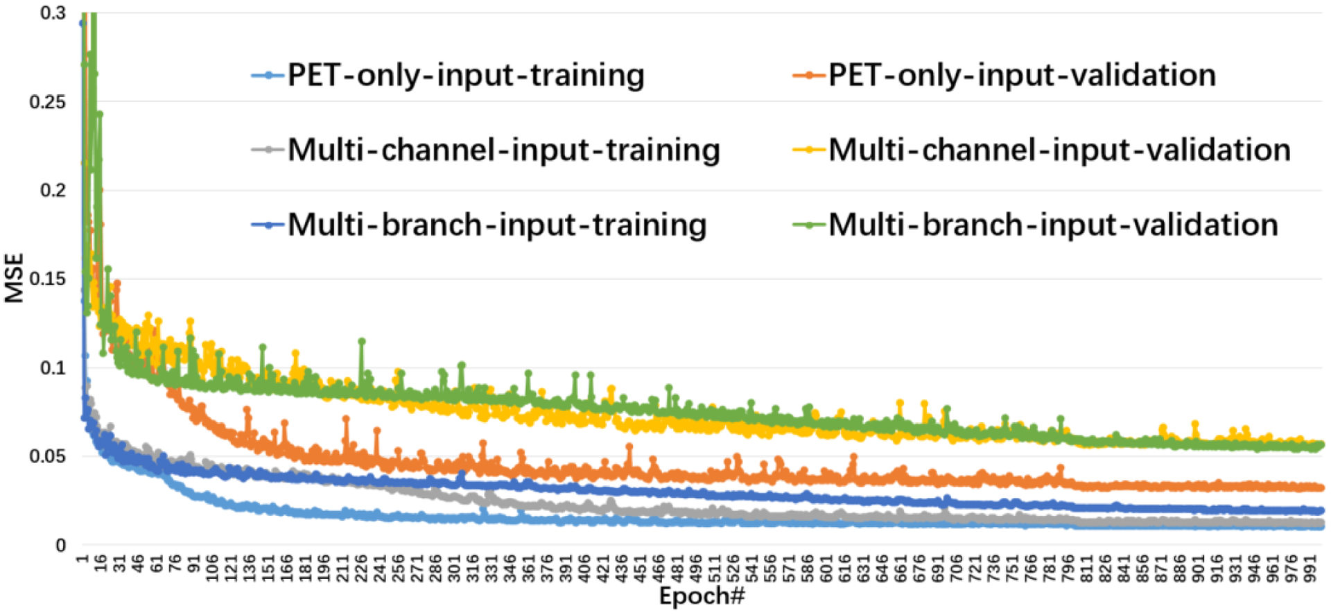
The training and validation losses as a function of epoch.
II.C. Data pre-processing
Prior to training, the CT image was downsampled using linear interpolation to match the PET pixel size and global registration was performed. In order to enhance soft-tissue contrast in CT images, we used the histogram equalization technique, which was performed using the function “histeq” in MATLAB. Essentially, the histogram equalization process finds a monotonic gray scale transformation such that the pixel intensities in the transformed image are uniformly distributed across the full gray scale. The image after histogram equalization would have a linearized cumulative distribution across the value range. Typical Hounsfield unit (HU) values of CT images are ranging from −1000 to 1000. In this paper, we add 1000 to the CT images and therefore the gray scale ranges from 0 to 2000. As shown in Fig.3, histogram equalization enhances soft-tissue contrast. Additionally, the intensity of CT and PET images are normalized by their own standard deviation. For a fair comparison, we use histogram equalized CT images in all anatomically aided reconstruction methods.
Figure 3:
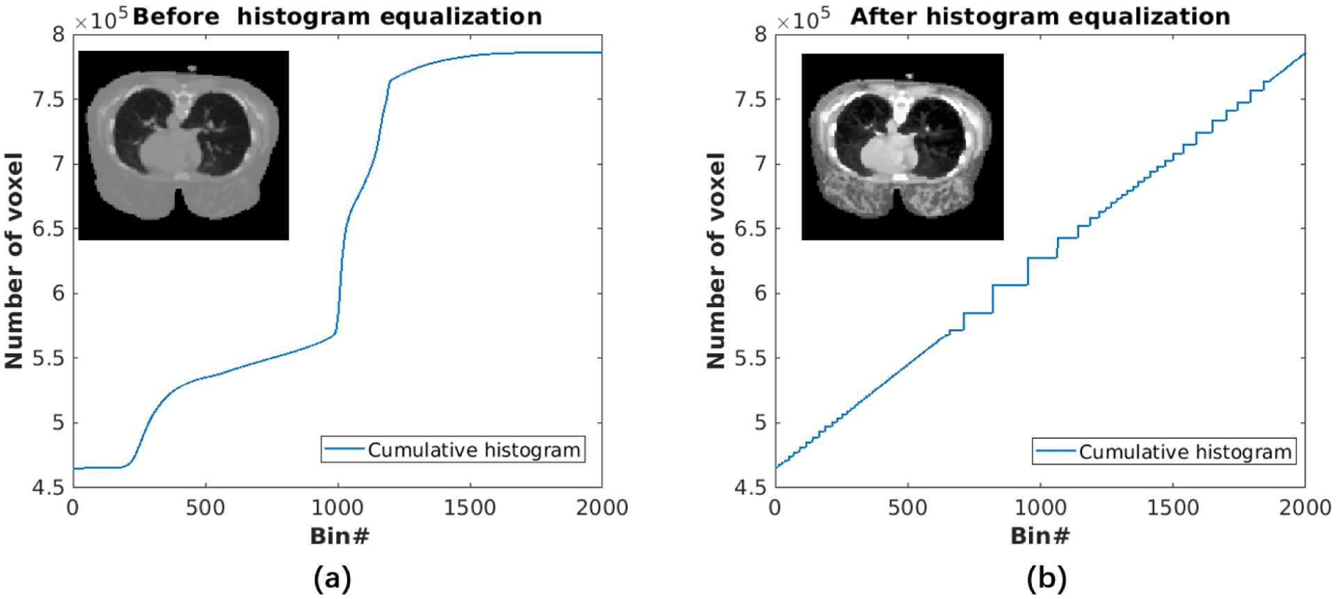
CT images and corresponding cumulative histogram (a) before and (b) after histogram equalization.
II.D. Reference Methods
In this study, we compared the proposed method with the kernel based reconstruction12, a state-of-the-art CNN-based regularized reconstruction48,49, and the iterative CNN constrained method published previously38.
Kernel method:
We used the CT image to generate a kernel matrix using a radial Gaussian function
| (14) |
where μi and μj are 3×3×3 local patches centered at voxel i and voxel j, respectively, in the CT image and Nf = 27 is the number of voxels in the patch. For efficient computation, all kernel matrices were constructed using a k-Nearest-Neighbor (kNN) search13 in a 7×7×7 search window with k = 30. Before feature extraction, CT images were normalized so that the image standard variation (σ) was equal to 1. The reconstructed image is then obtained by
| (15) |
which is solved by the kernel-EM algorithm12. This method is referred to as KEMCT.
Non–local meanpost–filtering method:
We applied non-local means (NLM) post-filtering to MLEM reconstruction. The filter kernel was built using the histogram-equalized CT images as described in equation (14). This method is referred to as NLM.
Deep penalty method:
We use the pre-trained CNN in the penalty function of a penalized ML reconstruction48,49. The reconstruction of the image x is formulated as the following optimization problem:
| (16) |
where x0 denotes an initial noisy reconstruction. The networks used in equation (16) are the same networks shown in Fig. 1 with either PET images only or PET/CT multi-modality images as the input. By using different networks, this method is denoted as DP-PET-only, DP-MC and DP-MB, respectively. Similar to equation (7), equation (16) with the quadratic prior can be solved by the optimization transfer method5.
Previous CNN constrained method:
This method represents the unknown PET image x by the output of a pre-trained CNN with PET only input without using anatomical information:
| (17) |
Similar to our proposed method, equation (17) is solved by ADMM38. This iterative CNN constrained method is denoted as ADMM-PET-only.
III. Experimental evaluations
III.A. Simulation Study
The computer simulation was used to evaluate the proposed method based on the geometry of a GE 690 scanner50. We simulated twenty XCAT51 phantoms (18 for training, 1 for validation and 1 for testing) with different organ sizes and genders. The image dimension and voxel size were 128 × 128 × 49 and 3.27 × 3.27 × 3.27 mm3, respectively. In the training datasets, 30 hot spheres were inserted in the lung region with diameters ranging from 12.8 mm to 22.1 mm. Similarly, we inserted two spherical lesions with diameters of 12.8 mm in the test phantom. The tissue specific time-activity curves were obtained using a compartmental model with kinetic parameters mimicking an 18F-FDG scan. Details of the simulation setup were described in our previous work38. The neural networks were trained with low-count reconstructions (4-min scans) as inputs and high-count reconstructions (40-min scans) as labels. Afterward, we quantitatively evaluated the performance of each method using the test phantom. The contrast recovery (CR) for the lesions vs. the background standard deviation (STD) curves were plotted. The CR was determined by
| (18) |
where is the uptake of the lung lesion in realization r, and is the true lesion uptake value. The total number of realizations is R = 10. The background STD was calculated as
| (19) |
where br,k is the average value of the kth background ROI in the rth realization and Kb = 20 is the number of 2D circular ROIs in each image. The background ROIs were manually drawn in the liver region across multiple axial slices.
III.B. Real patient studies
III.B.1. Hybrid lesion datasets
The hybrid lesion dataset consisted of 6 female patients (5 for training and 1 for testing), who received one-hour 18F-FDG dynamic scans on the GE Discovery 690 TOF-PET/CT scanner50 (GE Healthcare, Waukesha, WI, USA). The study was approved by the UC Davis Institutional Review Board. More patient information can be found in our previous work39. We generated high-count data using the measured events from 20 to 60 minutes post injection. Ten realizations of low-count data were obtained by randomly down-sampling the high-count data to 1/10th events. The reconstruction image dimension and voxel size were 180 × 180 × 49 and 3.27 × 3.27 × 3.27 mm3, respectively. For each realization, image augmentation was used by rotating the image with an angle randomly sampled between 0 and 90 degree39. The neural networks were trained with low-count reconstructions as inputs and high-count reconstructions as labels.
For quantitative analysis, spherical lesions with diameters of 13.1 mm and 16.4 mm were manually inserted into the testing data, but not into the training data. Lesion CR vs. background STD curves were obtained using the procedure described in Section III.A..
III.B.2. Lung cancer datasets
The lung cancer dataset included seven 18F-FDG patient scans (5 for training, 1 for validation and 1 for testing) from a Canon Celesteion TOF-PET/CT scanner52 (Canon Medical Corporation, Tochigi, Japan). Two 50% overlapping bed positions were acquired with 14 minutes per bed. The body weights distribution of patients was in a moderate range from 45 to 74 kg and the injected activity ranged from 160 to 250 MBq. The 14-minute scans were used as the high-count datasets and the low-count datasets were generated by downsampling the high-count datasets to 1/7th events. The same image augmentation procedure described above was used39. The reconstructed image dimension and voxel size were respectively 272 × 272 × 141 and 2.0 × 2.0 × 2.0 mm3. For quantitative analysis, liver ROIs were placed in a uniform area to calculate the STD. Although true lesion uptakes in real patient datasets were not known, we computed the CR based on the high-count reconstruction (100 MLEM iterations), which can serve as a reasonable surrogate of the ground truth.
IV. Results
IV.A. Simulation data
Fig. 4 shows transverse (top), coronal (middle), and sagittal (bottom) views of different reconstructed images through the lesion of interest. All of the methods are compared at a matched lesion contrast, indicated by the dashed black line in Fig. 5 (a). Both the NLM filter and the CT-aided kernel reconstruction demonstrated reduced noise and reduced partial volume effects (PVE), in comparison with the commonly used MLEM. Compared with the NLM filter, KEMCT can generate clearer myocardial structures with the help of the data consistency. Comparing images in fig 4(d)–(f) with those in fig 4(g,h,j), we can see that the results of CNN constrained reconstructions (ADMM-PET-only, ADMM-MC, ADMM-MB) have lower noise in the uniform region compared to their deep penalty counterparts (DP-PET-only, DP-MC, DP-MB). Comparing Fig. 4(i) with Fig. 4(j), we found that with histogram equalization, the myocardium boundary is more continuous and the liver region is smoother. We also computed the mean squared error (MSE) of the reconstructed test image with respect to the high-count reference image (HC-MLEM) as a function of iterations. The MSE curves in Fig. 5 (b) indicated that ADMM-MB has the lowest MSE.
Figure 4:
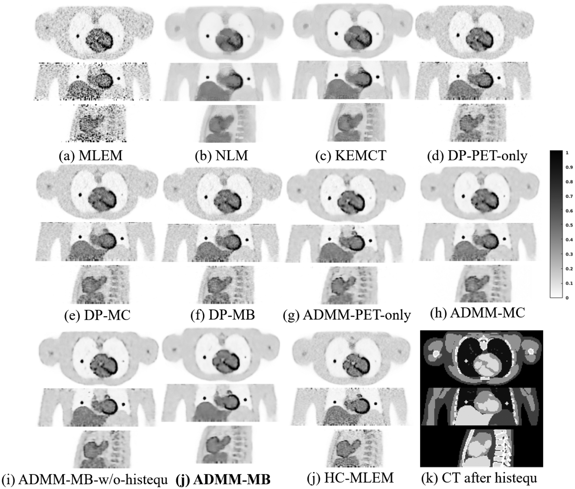
Reconstructed low-count images using different methods for the simulated test dataset. ADMM-MB-histequ denotes our proposed method method that uses the multi-branch input CNN constrained reconstruction with histogram equalized CT image. HC-MLEM represents MLEM reconstruction of high-count data for reference. Our proposed method is marked in bold face.
Figure 5:
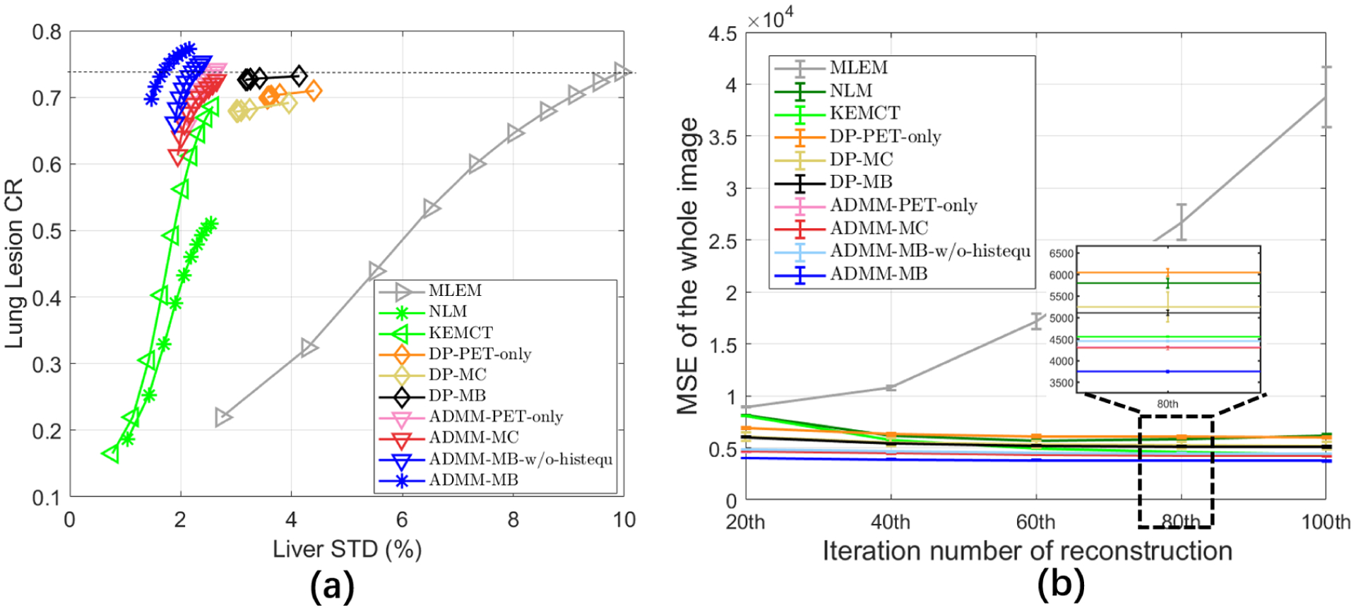
(a) The contrast recovery (CR) versus background standard derivation (STD) curves for the simulated test dataset. (b) The MSE as a function of iteration number for the simulated test dataset. Markers are plotted for every 10 iterations. Deep learning based methods were initialized with the 30th MLEM iteration.
From the CR vs. STD curves shown in Fig. 5, we see that the proposed iterative CNN constrained reconstruction with the multi-branch input outperforms all other methods with the highest CR at any matched STD level. In contast to the NLM method, both KEMCT and deep learning based reconstruction can better preserve lesions uptake. We can also see that both multi-channel input and multi-branch input have lower liver STD than the PET-only input result, although the difference between the CNN constrained reconstructions is relatively small. This finding indicates that the use of CT information in these methods can reduce noise in uniform soft-tissue regions. Including histogram equalization (ADMM-MB-histequ) also improves the convergence speed over using the CT image directly (ADMM-MB).
IV.B. Hybrid lesion datasets
Fig. 6 shows three orthogonal views of different reconstructed images through the lesion of interest. Similar to the simulation test dataset, all of the methods were compared at a matched lesion contrast, as indicated by the dashed black line in the CR vs. STD curves (Fig. 7). The CT-aided kernel reconstruction reduced noise and partial volume effects (PVE), in comparison with the commonly used MLEM. Compared with the deep penalty approaches, the CNN constrained reconstruction framework can recover more image details. Fig. 6 (c), (d), and (e) show that the deep penalty methods resulted in lower lung lesion contrast due to an increased smoothing across the images. The multi-channel network loses some fine details around the spine, as shown in Fig. 6 (d) and (g). Similar to KEMCT, the high activity region inside the bone marrow cannot be successfully identified.
Figure 6:
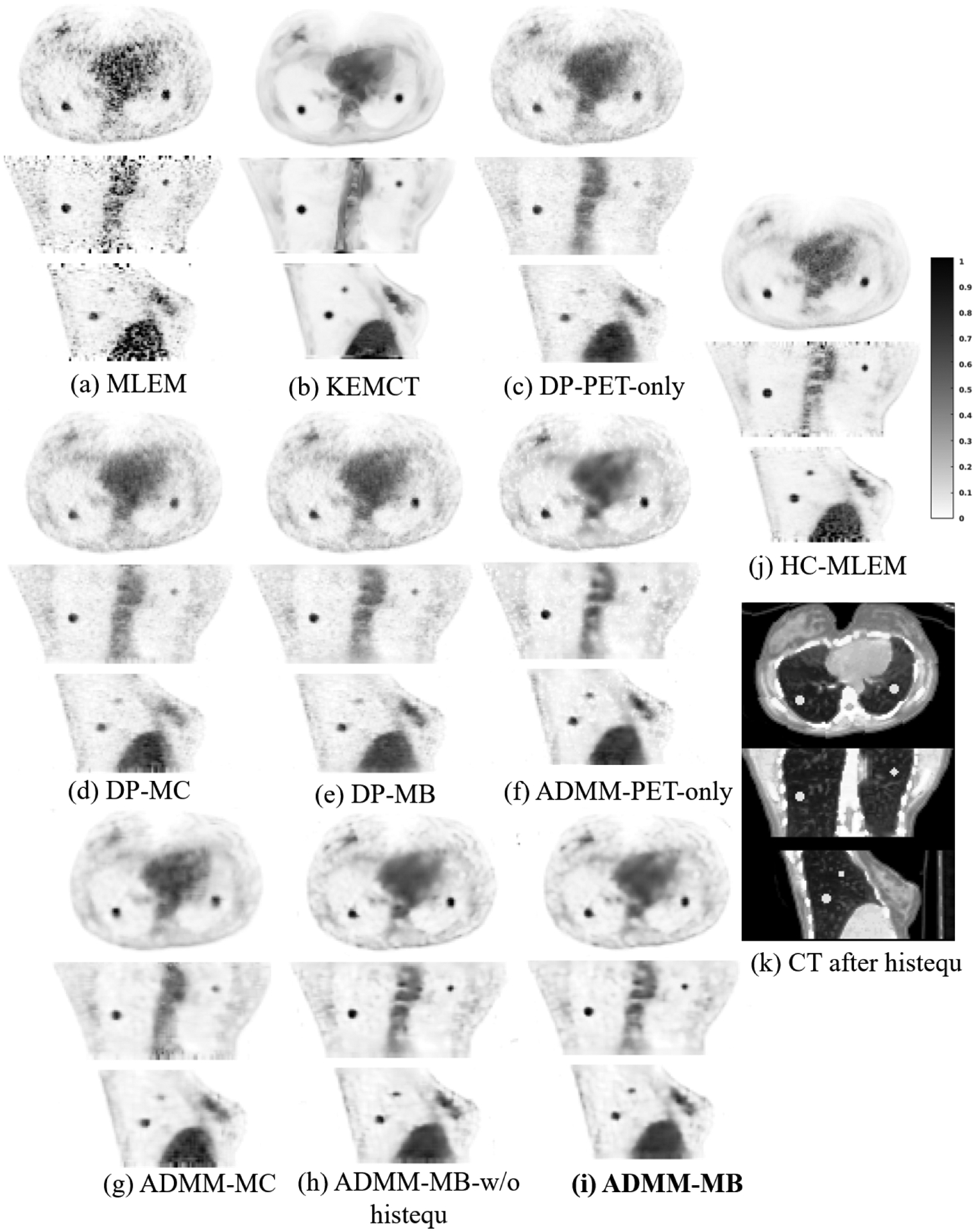
Reconstructed low-count images using different methods for the hybrid lesion test dataset. Our proposed method is marked in bold face. HC-MLEM denotes MLEM reconstruction of high-count data for reference.
Figure 7:
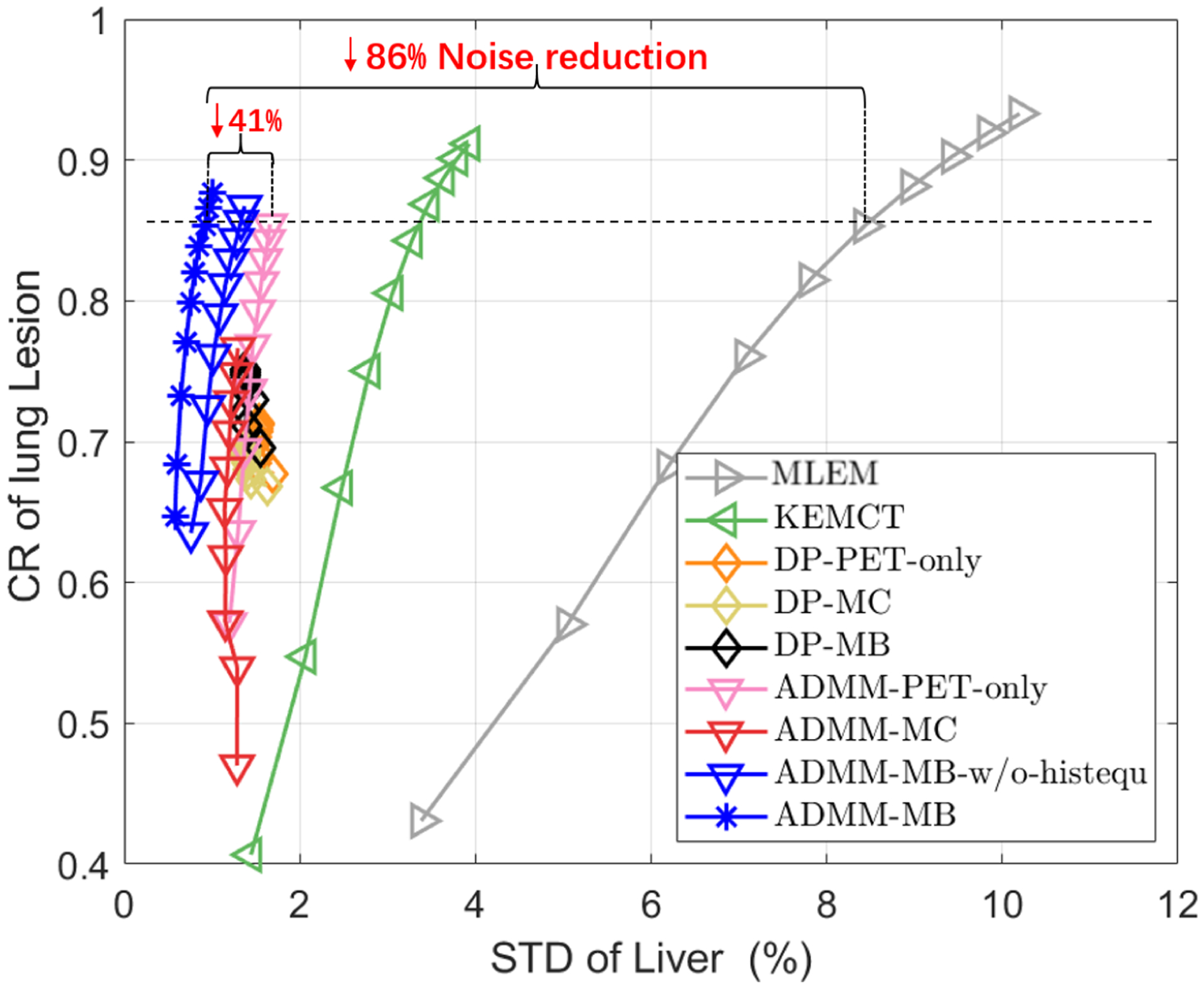
The contrast recovery (CR) versus background standard derivation (STD) curves for the hybrid lesion test dataset. Markers are plotted for every 10 iterations. Deep learning based methods were initialized with the 30th MLEM iteration.
In comparison, the multi-branch CNN constrained reconstruction holds the best CR-STD trade-off among all the methods. Fig. 7 demonstrates the proposed anatomy-aided CNN constrained reconstruction (ADMM-MB) can achieve better performance than KEMCT. After introducing histogram equalization, ADMM-MB-histequ converges faster and achieves a slightly better performance than ADMM-MB. Finally, compared with methods without using anatomical information, such as ADMM-PET-only and MLEM, our method can obtain 41% and 86% noise reduction, respectively, at matched CR levels.
IV.C. Lung cancer datasets
Fig. 8 shows the representative slices of reconstructed images and Fig. 9 shows the lung lesion contrast vs. liver STD curves for the test dataset. Using the KEMCT method (Fig. 8(b)), the noise has been suppressed but the lesion contrast is reduced. This is due to the imperfect registration between CT and PET. From our observations, there are some local mis-registrations between the CT and the PET, possibly due to repiratory motion. Compared with the KEMCT method, CNN constrained reconstruction achieved a higher lesion contrast while keeping a lower noise level. Moreover, ADMM-MB produces higher lesion contrast and has better noise tolerance than ADMM-PET-only. Similar to the results of hybrid lesion dataset, we also find that the liver is smoother in the anatomy-aided reconstructions compared to PET-only results (indicated by the black arrow). By visual inspection, our proposed method (ADMM-MB) has similar texture pattern compared to the high-count ML-EM reference. For instance, we can see that tumor activity in the lung is more uniformly distributed in the ADMM-MB method (Fig. 8(e)) compared to the ADMM-MB-w/o-histequ image (Fig. 8 (d)) and the ADMM-PET-only image (Fig. 8(c)).
Figure 8:
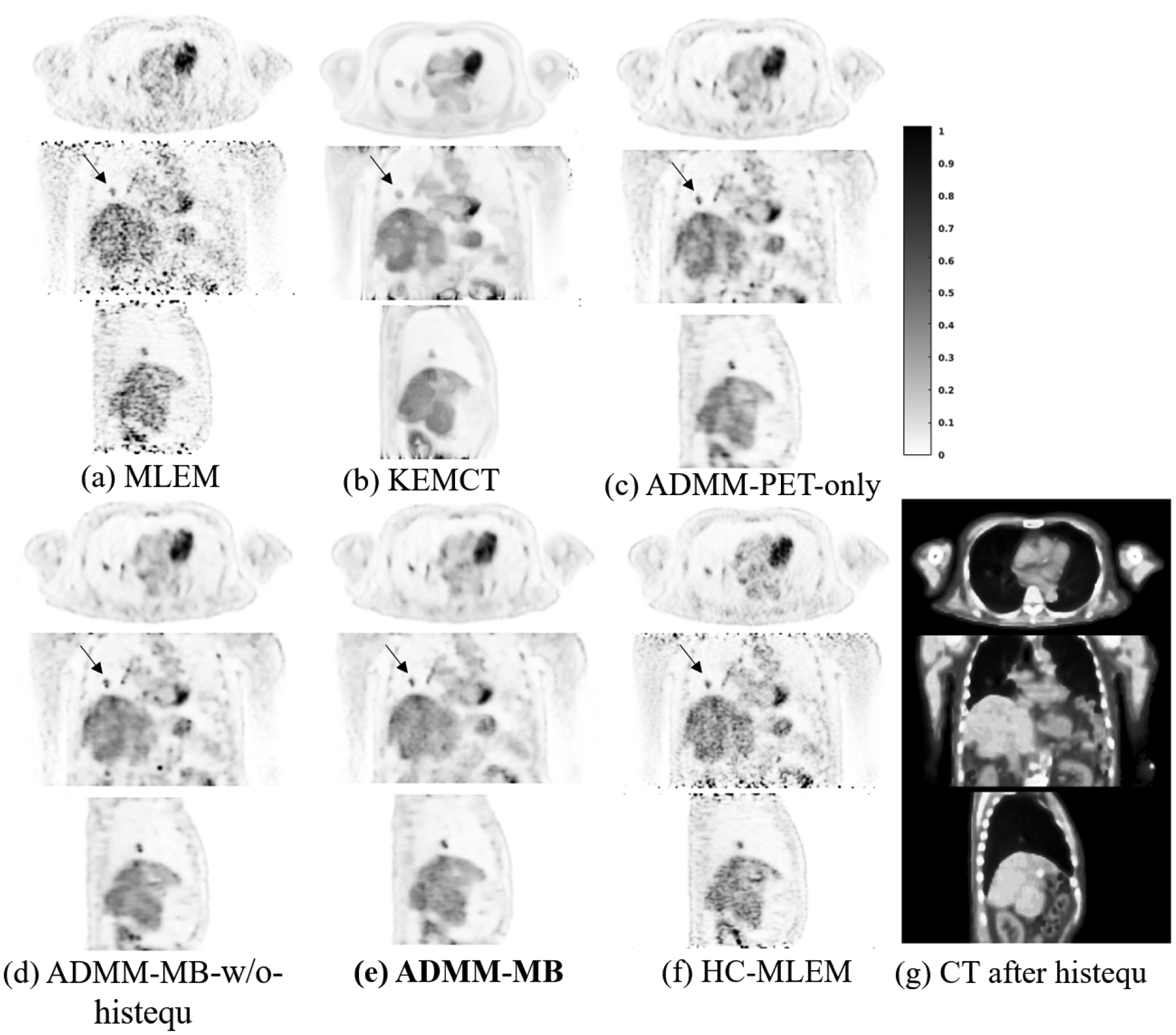
Reconstructed low-count images using different methods for the lung cancer test dataset. Our proposed method is marked in bold face. HC-MLEM denotes MLEM reconstruction of high-count data for reference.
Figure 9:
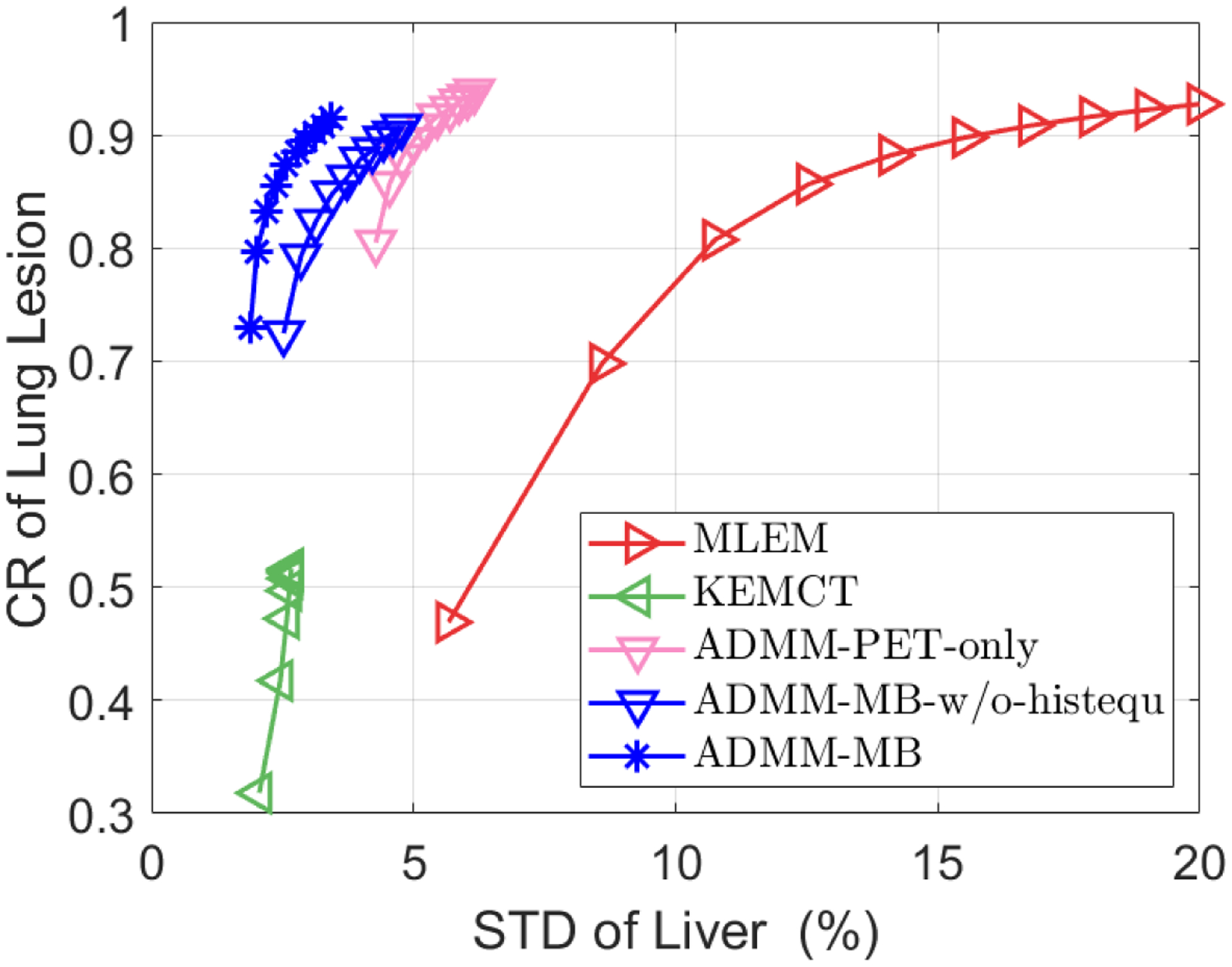
The contrast recovery (CR) versus background standard derivation (STD) curves for the lung cancer test dataset. Markers are plotted for every 10 iterations. Deep learning based methods were initialized with the 30th MLEM iteration.
V. Discussion
In this paper, we investigated two co-learning strategies for regularized PET image reconstruction. Our experimental results showed that the ADMM-MB-histequ outperformed existing methods, such as PET-only CNN-based reconstruction38 and anatomy-aided kernel reconstruction11. Although the KEMCT method has demonstrated reduced noise and reduced PVE properties, in practice, CT(only)-aided method is easily influenced by the mis-registration introduced by respiratory motion or the registration algorithm, as shown in the lung cancer dataset. In comparison, a deep network trained using real PET/CT images learns the mis-registration between low-count PET and CT inputs. Our experimental results demonstrated that the co-learning methods could compensate mismatch effects at least to some extent compared with KEMCT, as shown in Fig. 8.
Similar to previously reported methods16, the anato-functional methods which combine both anatomical and functional information, perform better than anatomy-aided only methods. It also should be noted that two co-learning strategies behave differently in terms of recovering small lesions, while both MC and MB have similar noise reduction ability. Without the help of modality-specific encoders, the multi-channel CNN combines both modalities in the first convolutional layer. However, as indicated by the metrics in Fig. 7 and the images in Fig. 6, this co-learning strategy tends to prioritize information from CT images at the expense of information from the PET data. A clear example is in the bone marrow, and only part of the bone marrow can be separated in DP-MC and ADMM-MC, because the tracer uptakes in the bone marrow are better separated in the PET image than in the CT image. Also the multi-channel network may not be able to fully learn the correlation between features in PET and CT images. To show that the improvement in performance was due to the change in network architecture, not simply by increasing the number of trainable parameters, we also trained a multi-branch network with 0.54 million parameters (8 root features). The new multi-branch network still outperformed the multi-channel network with 0.8 million parameters.
Compared with deep image prior based37 regularized reconstruction, our pre-trained network is capable of incorporating both inter-patient information and intra-patient information by learning from high-quality training samples. Additionally, the deep image prior method requires early stopping and the optimal iteration number is difficult to determine. In this paper, we do not introduce an extra likelihood function that encourages the network input to be similar to the unregularized ML reconstruction as we did in39, because we observed monotonic increase of L(y|α)) after incorporating the anatomical information. This indicates that with the introduction of anatomical information, pre-trained networks are less likely to generate undesirable outputs.
Another popular way of deep learning based reconstruction is the unrolling approach, which unrolls an iterative image reconstruction algorithm into a layer-wise structure and replaces certain components by neural networks. It often results in better interpretability. An unrolled network consists of series of modules, each having a regularization and data consistency unit. The number of trainable parameters increases with the number of modules if the network parameters are not shared among the modules53, and the GPU memory usage of the whole unrolled network can be huge. Furthermore, because the forward and back projections are embedded inside each module, the computational cost for an end-to-end training is extremely high. In comparison, we incorporate a pre-trained network in a constraint iterative reconstruction framework. The GPU memory usage is independent of iteration number, so we can use a deeper network. Also because the training does not involve any forward and back projection operations, the computational cost for training is much lower. Compared with unrolled methods, the performance of the ADMM in our method is sensitive to the hyperparameter ρ, which was manually adjusted in this work. How to address and alleviate this issue is of interest in our future studies.
One challenge in anatomically guided PET reconstruction is the potential mismatch between PET and CT images. We observed an example of a PET-unique lesion case in the validation data of the lung cancer dataset. As shown in Fig.10, the lesion can be barely identified in the CT image. Fig. 10(b) shows that KEMCT, which only uses CT information, has the worst lesion contrast. ADMM-PET-only performs better than ADMM-MB in terms of lesion contrast. However, ADMM-MB has a lower STD in the liver region at matched contrast level, which is mainly attributed to the much smoother background in CT images.
Figure 10:
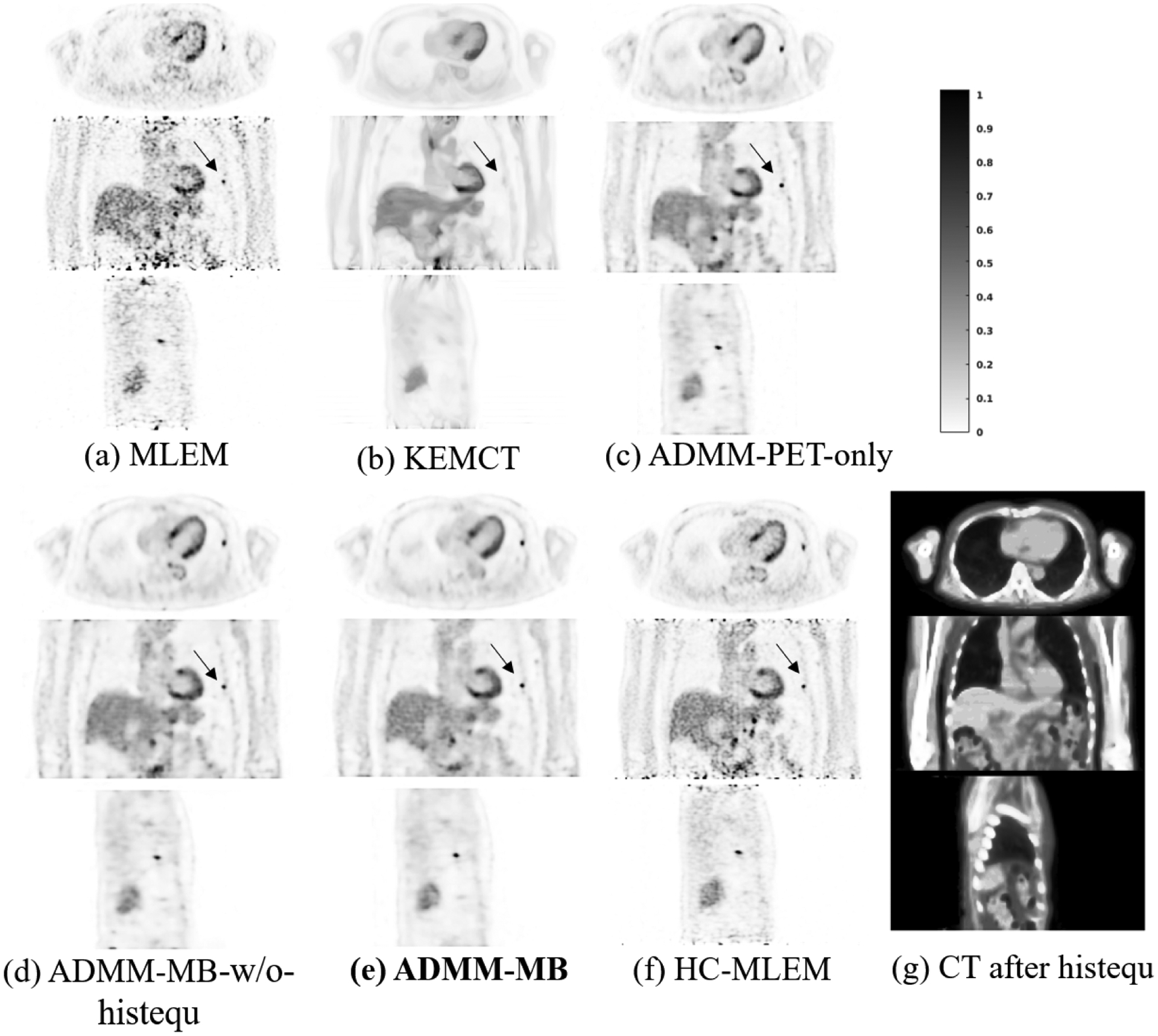
Reconstructed low-count images using different methods for the lung cancer validation dataset. Our proposed method is marked in bold face. HC-MLEM denotes MLEM reconstruction of high-count data for reference.
In this study, we trained two CNNs with datasets acquired on GE and Canon scanners separately. In a previous work54, we also tried to directly deployed the network trained using GE dataset to the Canon dataset. The results indicated a reasonable generalizability of the pre-trained network between inter-vendor scanners. Furthermore, integrating the deep neural network in iterative reconstruction can improve the image quality and reduce the variation between different networks. While we have only studied FDG PET scans so far, our reconstruction framework is applicable to other PET tracers. However, to achieve the best performance, additional fine tuning of the network parameters may be necessary for some PET tracers.
VI. Conclusion
In this work, we proposed an anatomy-aided PET image reconstruction method. By co-learning PET/CT information, the pre-trained deep neural network is used to represent PET images and to incorporate inter- and intra-patient information into PET image reconstruction. Evaluations using computer simulations and real datasets indicated that the proposed reconstruction method improved image quality and produced a better lesion contrast vs. background standard deviation trade-off curve compared existing methods, such as ML-EM reconstruction, kernel-based reconstruction and CNN-based penalized reconstruction with and without anatomical guidance.
Table 1:
The acronyms of different methods.
| Methods | Abbreviation | Histequ preprocessing | |
|---|---|---|---|
| Low count | |||
| High count MLEM | HC-MLEM | -- | |
| Low count MLEM | MLEM | -- | |
| Non-local mean post processing based on CT kernel | NLM | w/ | |
| CT kernel base reconstruction | KEMCT | w/ | |
| Deep penalty reconstruction base on PET-only input network | DP-PET-only | -- | |
| Deep penalty reconstruction base on multi-channel input network | DP-MC | w/ | |
| Deep penalty reconstruction base on multi-branch input network | DP-MB | w/ | |
| Deep penalty reconstruction base on PET-only input network | DP-PET-only | -- | |
| PET-only input network-based iterative reconstruction with input constrain | ADMM-PET-only | -- | |
| Multi-channel input network-based iterative reconstruction with input constrain | ADMM-MC | w/ | |
| Multi-branch input network-based iterative reconstruction with input constrain | ADMM-MB | w/ | |
| Multi-branch input network-based iterative reconstruction with input constrain | ADMM-MB-w/o-hisequ | w/o |
-- : The inputs do not include CT.
Table 2:
The summary of three datasets.
| Dataset | Scan time | Numbers of subject | Image dimension |
Voxel size (mm3) | ||
|---|---|---|---|---|---|---|
| Simulation | GE 690 geometry | Low count (20th, 30th, 50th MLEM iteration) |
4 min | 20 phantoms: 18 for training, 1 for validation, 1 for testing |
128 × 128 × 49 | 3:27 × 3:27 × 3:27 |
| High count (50th MLEM iteration) |
40 min | |||||
| Real patient | GE 690 | Low count (20th, 30th, 50th MLEM iteration) |
4 min | 6 patients: 5 for training, 1 for testing |
128 × 128 ×49 | 3:27 × 3:27 × 3:27 |
| High count (50th MLEM iteration) |
40 min | |||||
| Canon Celesteion | Low count (20th, 30th, 50th MLEM iteration) |
2 min | 7 patients: 5 for training, 1 for validation, 1 for testing |
272 × 272 × 141 | 2:0 × 2:0 × 2:0 | |
| High count (50th MLEM iteration) |
14 min |
Acknowledgments
This work was supported in part by the National Institutes of Health under Grant R21EB026668. The authors have no other conflicts to disclose.
Data Availability Statement
The authors are unable to share patient data at this time.
References
- 1.Gambhir SS, Molecular imaging of cancer with positron emission tomography, Nature Reviews Cancer 2, 683–693 (2002). [DOI] [PubMed] [Google Scholar]
- 2.Van Sluis J, De Jong J, Schaar J, Noordzij W, Van Snick P, Dierckx R, Borra R, Willemsen A, and Boellaard R, Performance characteristics of the digital Biograph Vision PET/CT system, Journal of Nuclear Medicine 60, 1031–1036 (2019). [DOI] [PubMed] [Google Scholar]
- 3.Cherry SR, Jones T, Karp JS, Qi J, Moses WW, and Badawi RD, Total-body PET: maximizing sensitivity to create new opportunities for clinical research and patient care, Journal of Nuclear Medicine 59, 3–12 (2018). [DOI] [PMC free article] [PubMed] [Google Scholar]
- 4.Sawatzky A, Brune C, Wubbeling F, Kosters T, Schafers K, and Burger M, Accurate EM-TV algorithm in PET with low SNR, in 2008 IEEE nuclear science symposium conference record, pages 5133–5137, IEEE, 2008. [Google Scholar]
- 5.Wang G and Qi J, Penalized likelihood PET image reconstruction using patch-based edge-preserving regularization, IEEE transactions on medical imaging 31, 2194–2204 (2012). [DOI] [PMC free article] [PubMed] [Google Scholar]
- 6.Sastry S and Carson RE, Multimodality Bayesian algorithm for image reconstruction in positron emission tomography: a tissue composition model, IEEE Transactions on Medical imaging 16, 750–761 (1997). [DOI] [PubMed] [Google Scholar]
- 7.Baete K, Nuyts J, Van Paesschen W, Suetens P, and Dupont P, Anatomical-based FDG-PET reconstruction for the detection of hypo-metabolic regions in epilepsy, IEEE transactions on medical imaging 23, 510–519 (2004). [DOI] [PubMed] [Google Scholar]
- 8.Bowsher JE, Johnson VE, Turkington TG, Jaszczak RJ, Floyd C, and Coleman RE, Bayesian reconstruction and use of anatomical a priori information for emission tomography, IEEE Transactions on Medical Imaging 15, 673–686 (1996). [DOI] [PubMed] [Google Scholar]
- 9.Tang J and Rahmim A, Bayesian PET image reconstruction incorporating anatofunctional joint entropy, Physics in Medicine & Biology 54, 7063 (2009). [DOI] [PMC free article] [PubMed] [Google Scholar]
- 10.Cheng-Liao J and Qi J, PET image reconstruction with anatomical edge guided level set prior, Physics in Medicine & Biology 56, 6899 (2011). [DOI] [PMC free article] [PubMed] [Google Scholar]
- 11.Hutchcroft W, Wang G, Chen KT, Catana C, and Qi J, Anatomically-aided PET reconstruction using the kernel method, Physics in Medicine and Biology 61, 6668 (2016). [DOI] [PMC free article] [PubMed] [Google Scholar]
- 12.Wang G and Qi J, PET image reconstruction using kernel method, IEEE Transactions on Medical Imaging 34, 61–71 (2015). [DOI] [PMC free article] [PubMed] [Google Scholar]
- 13.Gong K, Cheng-Liao J, Wang G, Chen KT, Catana C, and Qi J, Direct Patlak reconstruction from dynamic PET data using kernel method with MRI information based on structural similarity, IEEE transactions on medical imaging 37, 955–965 (2018). [DOI] [PMC free article] [PubMed] [Google Scholar]
- 14.Bai B, Li Q, and Leahy RM, Magnetic resonance-guided positron emission tomography image reconstruction, in Seminars in nuclear medicine, volume 43, pages 30–44, Elsevier, 2013. [DOI] [PMC free article] [PubMed] [Google Scholar]
- 15.Schramm G, Holler M, Rezaei A, Vunckx K, Knoll F, Bredies K, Boada F, and Nuyts J, Evaluation of parallel level sets and Bowsher’s method as segmentation-free anatomical priors for time-of-flight PET reconstruction, IEEE transactions on medical imaging 37, 590–603 (2017). [DOI] [PMC free article] [PubMed] [Google Scholar]
- 16.Bland J, Mehranian A, Belzunce MA, Ellis S, da Costa-Luis C, McGinnity CJ, Hammers A, and Reader AJ, Intercomparison of MR-informed PET image reconstruction methods, Medical physics 46, 5055–5074 (2019). [DOI] [PMC free article] [PubMed] [Google Scholar]
- 17.LeCun Y, Bengio Y, and Hinton G, Deep learning, nature 521, 436 (2015). [DOI] [PubMed] [Google Scholar]
- 18.Zhao X, Li L, Lu W, and Tan S, Tumor co-segmentation in PET/CT using multi-modality fully convolutional neural network, Physics in Medicine & Biology 64, 015011 (2018). [DOI] [PMC free article] [PubMed] [Google Scholar]
- 19.Kumar A, Fulham M, Feng D, and Kim J, Co-learning feature fusion maps from PET-CT images of lung cancer, IEEE Transactions on Medical Imaging 39, 204–217 (2019). [DOI] [PubMed] [Google Scholar]
- 20.Xiang L, Qiao Y, Nie D, An L, Lin W, Wang Q, and Shen D, Deep auto-context convolutional neural networks for standard-dose PET image estimation from low-dose PET/MRI, Neurocomputing 267, 406–416 (2017). [DOI] [PMC free article] [PubMed] [Google Scholar]
- 21.Liu C-C and Qi J, Higher SNR PET image prediction using a deep learning model and MRI image, Physics in Medicine & Biology 64, 115004 (2019). [DOI] [PMC free article] [PubMed] [Google Scholar]
- 22.da Costa-Luis CO and Reader AJ, Micro-networks for robust MR-guided low count PET imaging, IEEE Transactions on Radiation and Plasma Medical Sciences, 1–1 (2020). [DOI] [PMC free article] [PubMed] [Google Scholar]
- 23.Cui J et al. , PET image denoising using unsupervised deep learning, European journal of nuclear medicine and molecular imaging 46, 2780–2789 (2019). [DOI] [PMC free article] [PubMed] [Google Scholar]
- 24.Ulyanov D, Vedaldi A, and Lempitsky V, Deep image prior, in IEEE CVPR, pages 9446–9454, 2018. [Google Scholar]
- 25.Lei Y, Wang T, Dong X, Higgins K, Liu T, Curran WJ, Mao H, Nye JA, and Yang X, Low dose PET imaging with CT-aided cycle-consistent adversarial networks, in Medical Imaging 2020: Physics of Medical Imaging, volume 11312, page 1131247, International Society for Optics and Photonics, 2020. [Google Scholar]
- 26.Yang X, Lei Y, Fu Y, Wang T, Liu T, Higgins K, Curran W, Mao H, and Nye J, CT-aided Low-Count Whole-body PET Imaging Using Cross-Modality Attention Pyramid Network, Journal of Nuclear Medicine 61, 1416–1416 (2020). [Google Scholar]
- 27.Lei Y, Dong X, Wang T, Higgins K, Liu T, Curran WJ, Mao H, Nye JA, and Yang X, Whole-body PET estimation from low count statistics using cycle-consistent generative adversarial networks, Physics in Medicine & Biology 64, 215017 (2019). [DOI] [PMC free article] [PubMed] [Google Scholar]
- 28.Zhou L, Schaefferkoetter JD, Tham IW, Huang G, and Yan J, Supervised learning with CycleGAN for low-dose FDG PET image denoising, Medical Image Analysis, 101770 (2020). [DOI] [PubMed] [Google Scholar]
- 29.Antun V, Renna F, Poon C, Adcock B, and Hansen AC, On instabilities of deep learning in image reconstruction and the potential costs of AI, Proceedings of the National Academy of Sciences (2020). [DOI] [PMC free article] [PubMed] [Google Scholar]
- 30.Wang G, Ye JC, Mueller K, and Fessler JA, Image reconstruction is a new frontier of machine learning, IEEE transactions on medical imaging 37, 1289–1296 (2018). [DOI] [PubMed] [Google Scholar]
- 31.Ravishankar S, Ye JC, and Fessler JA, Image Reconstruction: From Sparsity to Data-Adaptive Methods and Machine Learning, Proceedings of the IEEE, 1–24 (2019). [DOI] [PMC free article] [PubMed] [Google Scholar]
- 32.Gong K, Berg E, Cherry SR, and Qi J, Machine Learning in PET: From Photon Detection to Quantitative Image Reconstruction, Proceedings of the IEEE 108, 51–68 (2020). [DOI] [PMC free article] [PubMed] [Google Scholar]
- 33.Zhu B, Liu JZ, Cauley SF, Rosen BR, and Rosen MS, Image reconstruction by domain-transform manifold learning, Nature 555, 487 (2018). [DOI] [PubMed] [Google Scholar]
- 34.Häggström I, Schmidtlein CR, Campanella G, and Fuchs TJ, DeepPET: A deep encoder–decoder network for directly solving the PET image reconstruction inverse problem, Medical image analysis 54, 253–262 (2019). [DOI] [PMC free article] [PubMed] [Google Scholar]
- 35.Kim K, Wu D, Gong K, Dutta J, Kim JH, Son YD, Kim HK, El Fakhri G, and Li Q, Penalized PET reconstruction using deep learning prior and local linear fitting, IEEE transactions on medical imaging 37, 1478–1487 (2018). [DOI] [PMC free article] [PubMed] [Google Scholar]
- 36.Sun J et al. , Deep ADMM-Net for compressive sensing MRI, in Advances in neural information processing systems, pages 10–18, 2016. [Google Scholar]
- 37.Gong K, Catana C, Qi J, and Li Q, PET image reconstruction using deep image prior, IEEE transactions on medical imaging 38, 1655–1665 (2018). [DOI] [PMC free article] [PubMed] [Google Scholar]
- 38.Gong K, Guan J, Kim K, Zhang X, Yang J, Seo Y, El Fakhri G, Qi J, and Li Q, Iterative PET image reconstruction using convolutional neural network representation, IEEE transactions on medical imaging 38, 675–685 (2019a). [DOI] [PMC free article] [PubMed] [Google Scholar]
- 39.Xie Z, Baikejiang R, Li T, Zhang X, Gong K, Zhang M, Qi W, Asma E, and Qi J, Generative adversarial network based regularized image reconstruction for PET, Physics in Medicine & Biology (2020). [DOI] [PMC free article] [PubMed] [Google Scholar]
- 40.Zhang W, Li R, Deng H, Wang L, Lin W, Ji S, and Shen D, Deep convolutional neural networks for multi-modality isointense infant brain image segmentation, NeuroImage 108, 214–224 (2015). [DOI] [PMC free article] [PubMed] [Google Scholar]
- 41.Teramoto A, Fujita H, Yamamuro O, and Tamaki T, Automated detection of pulmonary nodules in PET/CT images: Ensemble false-positive reduction using a convolutional neural network technique, Medical physics 43, 2821–2827 (2016). [DOI] [PubMed] [Google Scholar]
- 42.Boyd S et al. , Distributed optimization and statistical learning via the alternating direction method of multipliers, Foundations and Trends in Machine learning 3, 1–122 (2011). [Google Scholar]
- 43.Ronneberger O, Fischer P, and Brox T, U-net: Convolutional networks for biomedical image segmentation, in International Conference on Medical image computing and computer-assisted intervention, pages 234–241, Springer, 2015. [Google Scholar]
- 44.Zhang H, Goodfellow I, Metaxas D, and Odena A, Self-Attention Generative Adversarial Networks, arXiv preprint arXiv:1805.08318 (2018). [Google Scholar]
- 45.Oktay O et al. , Attention u-net: Learning where to look for the pancreas, arXiv preprint arXiv:1804.03999 (2018). [Google Scholar]
- 46.Xie Z, Baikejiang R, Gong K, Zhang X, and Qi J, Generative adversarial networks based regularized image reconstruction for PET, in 15th International Meeting on Fully Three-Dimensional Image Reconstruction in Radiology and Nuclear Medicine, edited by Matej S and Metzler SD, volume 11072, pages 114 – 118, International Society for Optics and Photonics, SPIE, 2019. [Google Scholar]
- 47.Kingma DP and Ba J, Adam: A method for stochastic optimization, arXiv preprint arXiv:1412.6980 (2014). [Google Scholar]
- 48.Wang S, Su Z, Ying L, Peng X, Zhu S, Liang F, Feng D, and Liang D, Accelerating magnetic resonance imaging via deep learning, in 2016 IEEE 13th International Symposium on Biomedical Imaging (ISBI), pages 514–517, IEEE, 2016. [DOI] [PMC free article] [PubMed] [Google Scholar]
- 49.Aggarwal HK, Mani MP, and Jacob M, MoDL: Model-based deep learning architecture for inverse problems, IEEE transactions on medical imaging 38, 394–405 (2018). [DOI] [PMC free article] [PubMed] [Google Scholar]
- 50.Bettinardi V, Presotto L, Rapisarda E, Picchio M, Gianolli L, and Gilardi M, Physical Performance of the new hybrid PET/CT Discovery-690, Medical physics 38, 5394–5411 (2011). [DOI] [PubMed] [Google Scholar]
- 51.Segars W, Sturgeon G, Mendonca S, Grimes J, and Tsui BM, 4D XCAT phantom for multimodality imaging research, Medical physics 37, 4902–4915 (2010). [DOI] [PMC free article] [PubMed] [Google Scholar]
- 52.Kaneta T, Ogawa M, Motomura N, Iizuka H, Arisawa A, Yoshida K, and Inoue T, Initial evaluation of the Celesteion large-bore PET/CT scanner in accordance with the NEMA NU2–2012 standard and the Japanese guideline for oncology FDG PET/CT data acquisition protocol version 2.0, EJNMMI research 7, 83 (2017). [DOI] [PMC free article] [PubMed] [Google Scholar]
- 53.Gong K, Wu D, Kim K, Yang J, El Fakhri G, Seo Y, and Li Q, Emnet: an unrolled deep neural network for pet image reconstruction, in Medical Imaging 2019: Physics of Medical Imaging, volume 10948, page 1094853, International Society for Optics and Photonics, 2019. [Google Scholar]
- 54.Xie Z, Li T, Zhang M, Qi W, Asma E, and Qi J, Deep learning based PET image reconstruction protocol for inter-vendor scanners, in IEEE Symposium Conference Record Nuclear Science 2019., 2019. [Google Scholar]
Associated Data
This section collects any data citations, data availability statements, or supplementary materials included in this article.
Data Availability Statement
The authors are unable to share patient data at this time.


