Dynamical consequences of sensory feedback in a half-center oscillator coupled to a simple motor system

Abstract

We investigate a simple model for motor pattern generation that combines central pattern generator (CPG) dynamics with a sensory feedback (FB) mechanism. Our CPG comprises a half-center oscillator with conductance-based Morris–Lecar model neurons. Output from the CPG drives a push–pull motor system with biomechanics based on experimental data. A sensory feedback conductance from the muscles allows modulation of the CPG activity. We consider parameters under which the isolated CPG system has either “escape” or “release” dynamics, and we study both inhibitory and excitatory feedback conductances. We find that increasing the FB conductance relative to the CPG conductance makes the system more robust against external perturbations, but more susceptible to internal noise. Conversely, increasing the CPG conductance relative to the FB conductance has the opposite effects. We find that the “closed-loop” system, with sensory feedback in place, exhibits a richer repertoire of behaviors than the “open-loop” system, with motion determined entirely by the CPG dynamics. Moreover, we find that purely feedback-driven motor patterns, analogous to a chain reflex, occur only in the inhibition-mediated system. Finally, for pattern generation systems with inhibition-mediated sensory feedback, we find that the distinction between escape- and release-mediated CPG mechanisms is diminished in the presence of internal noise. Our observations support an antireductionist view of neuromotor physiology: Understanding mechanisms of robust motor control requires studying not only the central pattern generator circuit in isolation, but the intact closed-loop system as a whole.

1. Introduction

Most peripheral axons carry sensory rather than motor information, but the role of sensory feedback in motor dynamics and control has been underemphasized. On the one hand, the importance of sensory feedback in motor control systems can hardly be overstated. For example, in a comprehensive study of the 350,000 axons emerging from the spinal cord to innervate the human arm, over 90% carried sensory information from the limb to central circuits and fewer than 10% conveyed motor information to the periphery [25]. In his founding treatise on cybernetics, Wiener emphasized the significance of sensory feedback (Chap. IV), as well as the analogy between control principles in biological and engineering automata (Introduction) [72]. On the other hand, physiologists studying control of rhythmic movements have put considerable effort toward understanding intrinsic dynamical properties of central circuitry, in isolation from peripheral dynamics. The existence of central pattern generators (CPGs) has been hypothesized for over a century [7,8] and demonstrated experimentally in the spinal cord of mammals [30] and of lamprey [31], in wingbeat control in insects [52], in control of swallowing in invertebrates [43] and in control of breathing [59].

Bässler observed that the mechanisms of rhythm generation in an intact neuromotor system could be distinct from those at work in an isolated subsystem extracted (whether mathematically or surgically) from the original intact system [2]. He distinguished the “pattern generator” (the intact system) from the “central pattern generator” (the isolated central circuit). This observation suggests the importance of studying both the isolated and the intact systems for rhythmic biological control, whether experimentally or through simulation and analysis.

In one such study, Kuo explored the relative contributions of feedforward and feedback pathways to robust rhythm generation in a simplified discrete-time version of a central pattern generator coupled to a push/pull motor system [37]. Kuo concluded that (i) purely feedforward systems were less robust against outside perturbations than systems incorporating sensory feedback from the periphery to central units and (ii) completely feedback-dependent systems (analogous to a chain reflex architecture) were less robust against sensory pathway noise. Moreover, in Kuo’s view, one may “interpret … the neural oscillator as a filter for processing sensory information rather than as a generator of commands.”

In this paper, we extend Kuo’s model from a discrete-time setting with impulsive motor action to a continuous-time system with rudimentary biomechanics. For concreteness, we incorporate length–tension properties measured in muscles from the feeding system in the marine mollusc Aplysia californica [75]. Kuo’s model combined a pendulum activated by opposing, alternating driving muscles. Here, we ask to what extent Kuo’s insights about the roles of feedforward and feedback signaling carry over to a continuous-time model for a CPG circuit coupled to a simple biomechanical system. To answer this question, we construct a simple brain–body system based on a half-center oscillator (HCO) model of the type studied by Zhang and Lewis [76] and introduced earlier by [57,58]. This HCO model incorporates two Morris–Lecar neurons [46] coupled by fast inhibitory synapses [60].

As observed in the earliest papers on half-center oscillators [57,58,68], the oscillation of the isolated circuit may be controlled by either of two complementary mechanisms. In a “release” mechanism, switching is triggered by a spontaneous decline in activity of the active cell, allowing the suppressed cell to become active. In an “escape” mechanism, spontaneous buildup of activity in the suppressed cell leads it to become active, thereby suppressing the previously active cell. Daun et al. investigated the different roles that release and escape transitions play in controlling the silent and active phase durations and oscillation periods in response to external drive modulation, and observed profound differences in sensitivity of the two mechanisms. In addition, they found that including adaptation currents leads to a blending of release and escape properties, with responses between the two extremes [14]. Subsequently, Zhang and Lewis noted different sensitivities to perturbations under the two mechanisms, reflected in the phase response curve [76].

The model we develop below leads to several conclusions. First, we confirm the broad outlines of Kuo’s analysis: increasing the strength of sensory feedback relative to the strength of coupling internal to the CPG generally increases the robustness of the system to external perturbations, in exchange for greater susceptibility to internal noise. Second, when sensory feedback is included in the model, it softens the distinction between the escape and release mechanisms. Specifically, the trade-off between sensitivity to internal versus external noise follows a similar pattern in the two cases, particularly when the feedback is mediated by inhibitory synapses. Finally, we observe that the closed-loop system incorporating sensory feedback exhibits a richer repertoire of dynamical behaviors than the purely feedforward CPG-driven system. In the model system studied here, we find that while the purely feedforward configuration produces symmetric periodic orbits (cf. Definition 1, p. 27), the configuration combining feedforward and feedback control exhibits both symmetric and nonsymmetric behaviors (cf. Definition 2, p. 27).

Together, these observations lend support to an antireductionist view of neuromotor physiology: Understanding mechanisms of robust motor control requires studying not only the central pattern generator circuit in isolation, but the intact closed-loop system as a whole [2,12,16,42,56].

2. Model

Our model falls within the framework proposed by [40,56] for studying the interaction of central nervous activity with biomechanics and sensory feedback, namely motor control models of the form

$$\frac{da}{dt}=f(a)+g(a,x),\frac{dx}{dt}=h(a,x)+\ell (x),$$ (1)

where a and x are the neural activity variables and body/motor variables, respectively, f represents the internal neural dynamics, h captures the biomechanics, g carries the sensory feedback and ℓ is an externally applied load. In this paper, we study unloaded motions, i.e., we set ℓ ≡ 0.

Figure 1 depicts the elements of our model: a CPG circuit coupled to a simple biomechanical system. The neural activity variables a in (1) correspond to the Morris–Lecar voltage and gating variables, {V₁, V₂, N₁, N₂}, and the body/motor variables x correspond to two muscle activation variables and the limb position, respectively, {A₁, A₂, x}.

Fig. 1.

Hybrid system combining central pattern generator (CPG), motor and feedback components. The CPG system comprises two mutually inhibitory Morris–Lecar neurons which produce a half-center oscillator pattern: Alternating bursts of activity driving opposite muscles. The muscles act on a limb with a 1D range of motion, shown here as a pendulum. Muscle stretch and contraction in turn produce reflex commands to feedback receptors and contralateral inhibition to neurons. Inhibitory connections end with a round ball, and excitatory connections end with a triangle

In the model, the HCO can have a release-type or an escape-type mechanism [57,68], and the sensory feedback can be ipsilateral or contralateral, excitatory or inhibitory, and activating or inactivating. Taking into account symmetries in the possible circuits, we reduce the possible configurations to four distinct variations, which we call inhibition-release, inhibition-escape, excitation-release and excitation-escape. In each case we presume contralateral, inactivating sensory feedback (see equation (18) for the full current balance model).

2.1. Half-center oscillator model

We study a central pattern generator (CPG) system comprising a “half-center oscillator” (HCO) consisting of two neurons connected by reciprocally inhibitory synapses. Following Skinner et al. [57,76], we use neurons based on the Morris–Lecar equations [46]. The model equations for cell 1 are

$$C\frac{d{V}_1}{dt}=I_{\text{ext}}-g_{\text{L}}\left(V_1-E_{\text{L}}\right)-g_{\text{Ca}}{M}_{\infty }\left(V_1\right)\left(V_1-E_{\text{Ca}}\right)-g_{\text{K}}{N}_1\left(V_1-E_{\text{K}}\right)-g_{\text{syn}}^{\text{CPG}}{S}_{\infty }^{\text{CPG}}\left(V_2\right)\left(V_1-E_{\text{syn}}^{\text{CPG}}\right),$$ (2)

$$\frac{d{N}_1}{dt}={\lambda }_N\left(V_1\right)\left(N_{\infty }\left(V_1\right)-N_1\right),$$ (3)

where V₁ is the membrane voltage for cell 1 and N₁ is the gating variable for potassium channels in cell 1. C is the capacitance; I_ext is an external or imposed current; g_L, g_Ca and g_K are the leak, calcium and potassium maximal conductances, respectively; and E_L, E_Ca and E_K are the corresponding reversal potentials. The functions M_∞ and N_∞ represent the voltage-dependent activation curves for the calcium and potassium conductances at steady state, respectively:

$$M_{\infty }\left(V_1\right)=\frac{1}{2}\left(1+\text{tanh}\left(\frac{V_1-E_1}{E_2}\right)\right),$$

$$N_{\infty }\left(V_1\right)=\frac{1}{2}\left(1+\text{tanh}\left(\frac{V_1-E_3}{E_4}\right)\right).$$ (4)

Here, E₁ describes the voltage at which the calcium conductance is half maximal, and E₂ determines the steepness of the calcium activation curve M_∞(V₁). E₃ and E₄ for potassium channels have the same meanings as E₁ and E₂. In equation (3), λ_N is the time constant for the potassium conductance activation, given by

$${\lambda }_N\left(V_1\right)={\varphi }_N\left(\text{cosh}\left(\frac{V_1-E_3}{2E_4}\right)\right),$$ (5)

where ϕ_N is the minimum rate constant for potassium channels opening. The activation dynamics of g_Ca is significantly faster than that of g_K, and we treat it as instantaneous. Following [76], we adopt parameters for which the isolated Morris–Lecar neuron (i.e., with $g_{\text{syn}}^{\text{CPG}}=0$) has a globally attracting fixed point at (V ≈ 13.3 mV, N ≈ 0.85), corresponding to a state of depolarization block [21,54]. Figure 2 shows the (V, N) plane for a single cell with $g_{\text{syn}}^{\text{CPG}}$ settozero.

Fig. 2.

(V, N) phase plane for a single Morris–Lecar model neuron. Green solid line: N-nullcline (invariant as $g_{\text{syn}}^{\text{CPG}}$ varies). Red solid line: V-nullcline for the isolated cell, i.e., when $g_{\text{syn}}^{\text{CPG}}=0$. Solid black line: trajectory from an arbitrary initial point V₀ = −50, N₀ = 0.1 when $g_{\text{syn}}^{\text{CPG}}=0$. The trajectory converges to a globally attracting stable fixed point (black dot) which is the intersection of the V-nullcline and N-nullcline. Blue solid line: inhibited cell’s V-nullcline with CPG synaptic conductance $g_{\text{syn}}^{\text{CPG}}$ set to 0.008 and S_∞ ≡ 1. Black dashed line: trajectory from the same initial point when $g_{\text{syn}}^{\text{CPG}}=0.008$. In this example, the trajectory of the full model converges to a symmetric stable limit cycle

For the reciprocally inhibitory coupling, the fast synaptic current imposed by cell 2 on cell 1 is

$$g_{\text{syn}}^{\text{CPG}}{S}_{\infty }^{\text{CPG}}\left(V_2\right)\left(V_1-E_{\text{syn}}^{\text{CPG}}\right),$$ (6)

where $g_{\text{syn}}^{\text{CPG}}$ is the maximal CPG synaptic conductance and $E_{\text{syn}}^{\text{CPG}}$ is the reversal potential of the CPG conductance. The CPG synaptic activation is also assumed to be instantaneous and is given by the monotonically increasing sigmoidal function

$$S_{\infty }^{\text{CPG}}\left(V_2\right)=\frac{1}{2}\left(1+\text{tanh}\left(\frac{V_2-E_{\text{thresh }}}{E_{\text{slope }}}\right)\right),$$ (7)

where E_thresh is the voltage at which half of the CPG synaptic channels are open at steady state and E_slope determines the steepness of the CPG synaptic activation curve $S_{\infty }^{\text{CPG}}\left(V_2\right)$. Note that $g_{\text{syn }}^{\text{CPG}}{S}_{\infty }^{\text{CPG}}>0$, so that as long as $V_1>E_{\text{syn}}^{\text{CPG}}$, the CPG synaptic drive current gives a negative contribution to V₁.

The model equations for cell 2 are identical, after exchanging the subscript of variables, mutatis mutandis. Thus, our CPG model has the mirror symmetry typical of half-center oscillator models: the equations are equivariant with respect to interchanging of the labels 1 ↔ 2. See Sect. 4.1 for further discussion of model symmetries.

The HCO consists of two nonoscillatory neurons that are connected by reciprocally inhibitory synapses, as described above. The rapid calcium current kinetics and the fast synaptic CPG inhibition interact with the slow potassium current kinetics to produce anti-phase oscillations, so that the neurons periodically transition between an active state and a suppressed state. If the neurons’ transition between the two states is triggered by changes in the active neuron, the underlying mechanism is called “release.” If the transition is triggered by changes in the suppressed cell, it is called “escape” [57,60]. To be specific, for the release-type HCO, the cells’ transition between the active and suppressed states does not depend on the intrinsic dynamics of the suppressed cell. Instead, the timing of transition is controlled by the membrane potential of the active cell falling below the synaptic threshold E_thresh and releasing the suppressed cell from inhibition. On the other hand, for the escape-type HCO, the dynamics of the active cell and the synaptic threshold do not play a role in initiating the transition of the cells between the active and suppressed states; the timing of the transition is controlled by the intrinsic properties of the suppressed cell. That is, as the potassium gating variable of the suppressed cell drops below the escape threshold, the fast inward current overcomes the slow outward current, leading to a rapid depolarization of the suppressed cell and its escape from inhibition.

2.2. Muscle model

We couple the HCO to a simple biomechanical system, following the modeling framework developed in [75]. That is, we use a Hill-based kinetic model for smooth muscle in which the muscle force F is the product of three biomechanical factors: activation dynamics, length/tension properties and force/velocity properties, i.e.,

$$F(t)=F_0\cdot a(t)\cdot FV(v(t))\cdot LT(L(t)),$$ (8)

where F₀ is a scaling factor, a is the neurally controlled activation, FV is the force–velocity function of the muscle velocity υ and LT is the length–tension function of the muscle length L, measured in millimeters.

Yu et al. measured these factors for one the I2 muscle of the buccal mass from the marine mollusc Aplysia californica [75]. Since muscle velocity only influences the rate of change of the muscle force, but not its steady state (Fig. 4 in [75]), we make the simplifying assumption that the force–velocity relationship is a constant function,

$$FV(v)=1.$$ (9)

Therefore, the muscle force is given by

$$F(t)=F_0\cdot a(t)\cdot LT(L(t)).$$ (10)

In [75], the length–tension curve was modeled as a quadratic function¹

$$LT\left(L\right)=-\left(5.27\times {10}^{-4}\right){\left(L/\mathcal{l}\right)}^2+0.1054(L/\mathcal{l})-4.27,$$ (11)

and activation dynamics was modeled as a first-order low-pass filter, described by the following equations

$$U(t)=\left(1.03-4.31e^{(-0.198u(t))}\right)\Theta (u(t)-8),$$ (12)

$$\frac{dA(t)}{dt}={\tau }^{-1}\left\{U(t)-[\beta +(1-\beta )U(t)]A(t)\right\},$$ (13)

$$a(t)=g{\left[A(t)-a_0\right]}_{+}.$$ (14)

Here, Θ is the Heaviside step function and [u]₊ = uΘ(u). We assume that the neural input to the corresponding muscle in our model is $u=\frac{1}{2}V$.² The neural input u(t) is scaled in (12) by a nonlinear force–frequency relationship to U(t). The isometric force–frequency relationship of I2 has a frequency threshold of about 6–8 Hz, and thus, U is set to be initiated as u reaches 8 Hz. A nonlinear differential equation (13) gives the dynamic properties, relating the (unitless) internal variables U and A. The parameters τ and β are time constants of isometric force development. The final nonlinearity, (14), requires an excitation threshold a₀ to prevent negative forces at low frequencies, and the scale factor g is used to normalize the output.

Fig. 4.

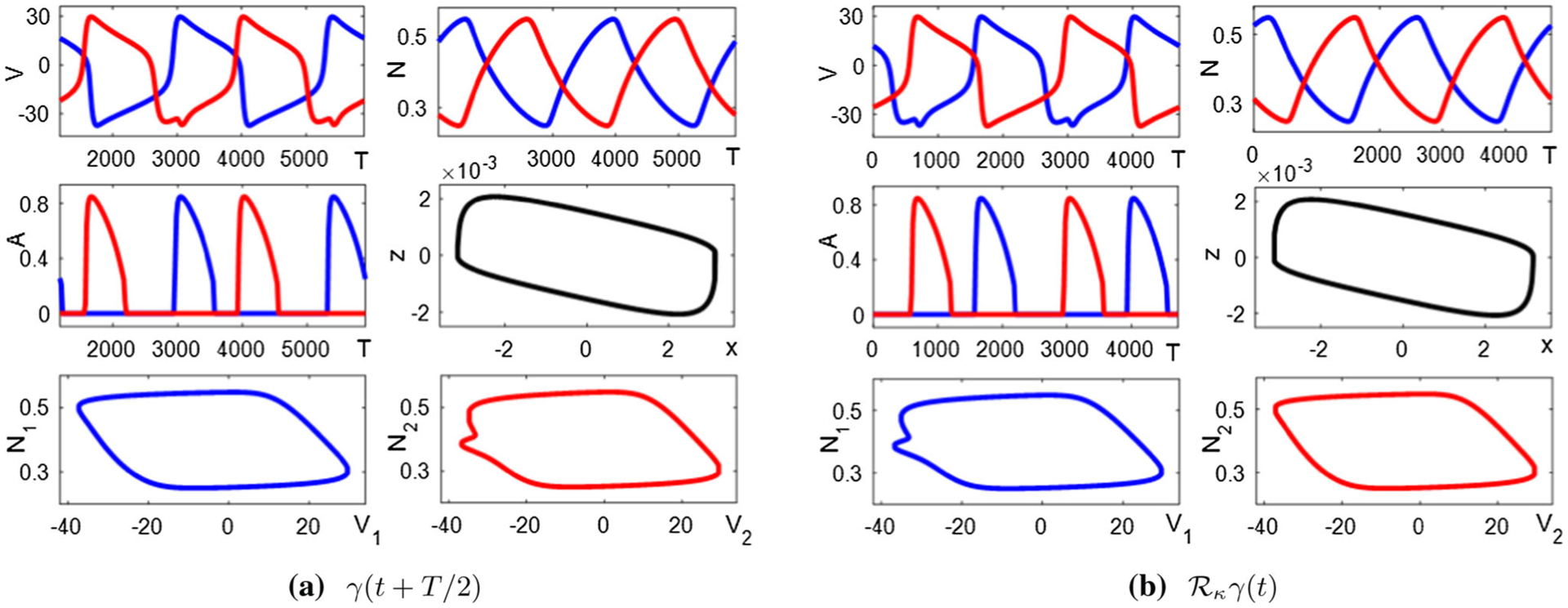
Inhibition-release mechanism (see Sect. 3.3) with $g_{\text{syn }}^{\text{CPG}}=0.008$ and $g_{\text{syn}}^{\text{FB}}=0.008$ has an asymmetric limit cycle solution with T ≈ 2361. a Components of the limit cycle γ (t) after a half-period shift. Blue trace: cell/muscle 1. Red trace: cell/muscle 2. Black trace: position (x) and velocity (z). b Components of γ after reflection operation, illustrating that ${\mathcal{R}}_{\kappa }\gamma (t)\ne \gamma (t+T/2)$ (see Sect. 4.1). Colors as in a

For mathematical convenience, Kuo employed a damped pendulum suspended between the two muscles under the influence of short bursts from muscular activity [37]. We adopt Kuo’s geometry and assume for simplicity that the relation between the pendulum position, x, and muscle lengths, L₁ and L₂, are linear:

$$L_1=(50+0.8x)\ell ,L_2=(50-0.8x)\ell ,-50<x<50,$$ (15)

where ℓ = 1 mm sets a nominal length scale. The dimensionless position x is described by

$$\frac{dx}{dt}=\frac{F_2-F_1}{b\ell },$$ (16)

where b is the friction coefficient and F_i (i = 1, 2) is the force applied to the pendulum by muscle i.

Sensory feedback from the “body” to the “brain” takes the form of feedback currents induced by the biomechanical system on the CPG circuit,

$$g_{\text{syn}}^{\text{FB}}{S}_{\infty }^{\text{FB}}\left(L_2\right)\left(V_1-E_{\text{syn}}^{\text{FB}}\right),g_{\text{syn}}^{\text{FB}}{S}_{\infty }^{\text{FB}}\left(L_1\right)\left(V_2-E_{\text{syn}}^{\text{FB}}\right),$$ (17)

where $g_{\text{syn}}^{\text{FB}}$ is the maximal feedback synaptic conductance and $E_{\text{syn}}^{\text{FB}}$ is the reversal potential of the feedback conductance. The sign of $E_{\text{Syn}}^{\text{FB}}\left(\left|E_{\text{syn}}^{\text{FB}}\right|=80\right)$ determines whether the feedback current is inhibitory (−) or excitatory (+) to the neuron. We assume that the feedback conductance has fast dynamics, so that it is taken to be an instantaneous function relative to the muscle length. In principle, the sensory feedback from a muscle could be imposed on either the ipsilateral or contralateral neuron in the CPG. Equation (17) represents the effect on the contralateral side. If acting on the ipsilateral neurons, the feedback current becomes $g_{\text{syn}}^{\text{FB}}{S}_{\infty }^{\text{FB}}\left(L_i\right)\left(V_i-E_{\text{syn}}^{\text{FB}}\right)$ (i = 1, 2). Furthermore, the feedback current channels might open when the corresponding muscle is either contracted or stretched; these two cases are represented either by a monotonically decreasing sigmoidal function $S_{\infty }^{\text{FB}}\left(L_i\right)=1-\frac{1}{2}\text{tanh}\left(\frac{L_i-x_0\ell }{L_{\text{slope}}}\right)$ (inactivating) or else by an increasing sigmoidal function $S_{\infty }^{\text{FB}}\left(L_i\right)=\frac{1}{2}\left(1+\text{tanh}\left(\frac{L_i-x_0\ell }{L_{\text{slope}}}\right)\right)$ (activating), respectively. Here, x₀ is the initial position of the pendulum, and L_slope determines the steepness of the feedback synaptic activation curves $S_{\infty }^{\text{FB}}\left(L_i\right)$. Taking these alternatives into account, there are prima facie sixteen possible variations of the neuromechanical system architecture: The HCO could be release-mediated or escape-mediated; the feedback current could be inhibitory or excitatory; the feedback current imposed on the neuron could come from the contralateral or ipsilateral muscle; and the feedback current could be activating or inactivating. In Sect. 3.2, we will explain how these sixteen possibilities reduce effectively to four functionally distinct scenarios. Figure 1 illustrates one of these cases: an inhibition-contralateral-inactivating system.

With sensory feedback incorporated into the model, we arrive at the full dynamics of the membrane voltage V_i (i ≠ j):

$$C\frac{d{V}_i}{dt}=I_{\text{ext}}-g_{\text{L}}\left(V_i-E_{\text{L}}\right)-g_{\text{Ca}}{M}_{\infty }\left(V_i\right)\left(V_i-E_{\text{Ca}}\right)-g_{\text{K}}{N}_i\left(V_i-E_{\text{K}}\right)-g_{\text{syn}}^{\text{CPG}}{S}_{\infty }^{\text{CPG}}\left(V_j\right)\left(V_i-E_{\text{syn}}^{\text{CPG}}\right)-g_{\text{syn}}^{\text{FB}}{S}_{\infty }^{\text{FB}}\left(L_j\right)\left(V_i-E_{\text{syn}}^{\text{FB}}\right).$$ (18)

The full seven-variable model (V₁, V₂, N₁, N₂, A₁, A₂, x) has the mirror symmetry typical of half-center oscillator based CPG systems. The ordinary differential equations are equivariant with respect to exchange of indices 1 ↔ 2 together with the reflection x ↔ −x. See Sect. 4.1 for further discussion of model symmetries. We solve the differential equations (3), (13), (16) and (18) numerically using MATLAB. Appendix A specifies parameter values used for simulations, and Appendix B lists the model equations discussed above and provides a link to the simulation codes, available through https://github.com/zhuojunyu-appliedmath/CPG-FB/.

3. Results

3.1. Symmetric and nonsymmetric trajectories

Like other central pattern generator models based on a hal-fcenter oscillator circuit, the model has a simple form of symmetry: Exchanging the labels “1” and “2” and reversing the sign of x leave the equations unchanged. In a dynamical system with mirror symmetry, we can also classify periodic orbits according to their symmetry. We observe two types of limit cycles occurring in our system: symmetric and nonsymmetric (see Sect. 4.1 for precise definitions). In a symmetric solution, the trajectory and its mirror image are identical after a time delay of one half period. In a nonsymmetric solution, the trajectory and its half-period delayed mirror image are different from one another. Figure 3 shows an example of a symmetric solution. As an example of a nonsymmetric solution, Fig. 4 shows a period-T trajectory in which the active phase of cell 1 (V₁ > V₂) lasts longer than T/2 time units, and the active phase of cell 2 (V₂ > V₁) has duration less than T/2. In our model, such pairs of asymmetric limit cycle solutions bifurcate from a single symmetric limit cycle solution via a pitchfork bifurcation under several circumstances, which is discussed below. We discuss the possible biological significance of symmetric vs. nonsymmetric solutions in Sect. 5.

Fig. 3.

Inhibition-release mechanism (see Sect. 3.3) with $g_{\text{syn}}^{\text{CPG}}=0.008$ and $g_{\text{syn}}^{\text{FB}}=0.006$ has a symmetric limit cycle solution with T ≈ 2254. a Components of the limit cycle γ (t). Blue trace: cell/muscle 1. Red trace: cell/muscle 2. Black trace: position (x) and velocity (z). b Components of γ after a half-period shift and reflection operation, illustrating that ${\mathcal{R}}_{\kappa }\gamma (t)=\gamma (t+T/2)$ (see Sect. 4.1). Colors as in a

3.2. Equivalent architectures

In order to study how movement generation is influenced by the relative strength of CPG-based and feedback-based rhythm-generating mechanisms, we focus on two key parameters: the CPG synaptic conductance, $g_{\text{syn }}^{\text{CPG }}$, and the feedback synaptic conductance, $g_{\text{syn}}^{\text{FB}}$, and ask how these conductances affect the oscillations produced by the system. Although the synaptic architecture affords sixteen superficially distinct variations, many of them are functionally equivalent. That is, we find empirically that the range of synaptic CPG and feedback conductances which can sustain steady oscillations are qualitatively similar despite changes in contralateral vs. ipsilateral feedback and in activating vs. inactivating feedback. This qualitative behavior is consistent with the observation that whether the muscles’ contraction or stretching activates the feedback current does not affect the topology of the brain–body circuit; neither does the contralateral versus ipsilateral muscle triggering the feedback current. Consequently, the sixteen different configurations fall into four functionally equivalent subgroups, which we call inhibition-release (IR), inhibition-escape (IE), excitation-release (ER), and excitation-escape (EE). Figure 5 illustrates our classification. For each of these four classes of architecture, we study the range for oscillation, the oscillation period, the limit cycle stability, and identify bifurcations, as functions of $g_{\text{syn}}^{\text{CPG}}$ and $g_{\text{syn}}^{\text{FB}}$. Moreover, we study the response of the systems when subjected to external perturbation and to internal noise.

Fig. 5.

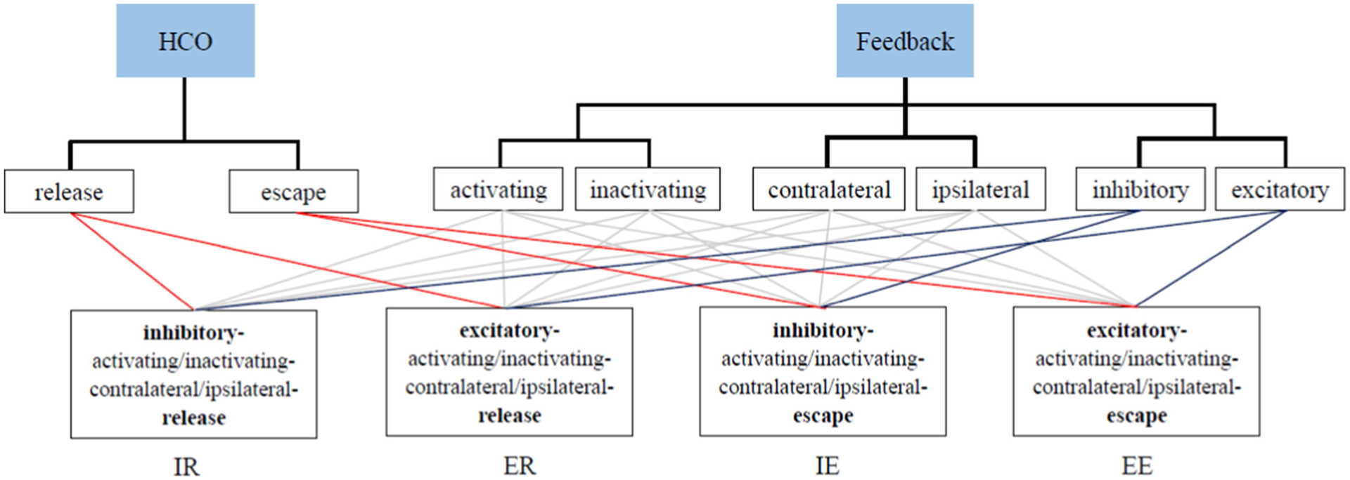
Although the CPG–motor system model has in principle sixteen different variants, we find empirically that they fall into four functionally equivalent architectures with qualitatively similar behavior (not shown), which we call inhibition-release (IR), excitation-release (ER), inhibition-escape (IE), excitation-escape (EE). Each distinct scenario includes four qualitatively similar cases. For example, in the left bottom block (IR), the four cases are inhibitory-activating-contralateral-release, inhibitory-inactivating-contralateral-release, inhibitory-activating-ipsilateral-release and inhibitory-inactivating-ispilateral-release

It is worth noting that when both the CPG conductance and the feedback conductance are removed, the system does not oscillate; the individual Morris–Lecar neurons are uncoupled and each has a stable fixed point (Sect. 2.1, Fig. 2). The eigenvalues of the isolated single-cell systems at the fixed point are strictly negative; therefore, there should exist an open set in parameter space in which the stable fixed point remains globally attracting. Thus, for the parameters we consider, rhythm generation depends on having either nonzero CPG conductance (the purely feedforward central pattern generator scenario), or nonzero feedback conductance (the pure “chain reflex” scenario) or a combination of both (the hybrid scenario).

3.3. Inhibition-release

The inhibition-release system cannot sustain oscillations with excessively large feedback conductance ($g_{\text{syn}}^{\text{FB}}\gtrsim 0.012\mu \text{S}/{\text{cm}}^2$). In contrast, the oscillations persist over a large range of the CPG conductance (up to 1 μS/cm²). Here, we focus on a range where the CPG and FB conductances are of comparable size, $0\le g_{\text{syn}}^{\text{FB}}\lesssim 0.012$ μS/cm², and $0\le g_{\text{syn}}^{\text{CPG}}\lesssim 0.014$ μS/cm². Within this range, we investigate how the oscillation period and the magnitude of the leading nontrivial Floquet multiplier vary over the two conductances (Fig. 6). These and subsequent results are computed using our model implemented in MatCont, and some of them are also tested through MATLAB. The method and its principles are explained in Sect. 4.

Fig. 6.

Oscillation period and the magnitude of the second Floquet multiplier of the inhibition-release mechanism. a Period. b Next-to-largest magnitude Floquet multiplier

Kuznetsov classified codimension-1 bifurcations of cycles in ${\mathbb{Z}}_2$-equivariant systems and gave sufficient conditions for fold, pitchfork and torus bifurcations in terms of the leading nontrivial Floquet multiplier(s) (μ₁, if real, or μ_1,2, if a complex conjugate pair) and normal forms in [38]. For a symmetric cycle (cf. Definition 1, p. 27), only the cases μ₁ = 1 and μ_1,2 = e^±iθ have to be considered: Fold and pitchfork bifurcations occur at μ₁ = 1, which is the only nontrivial multiplier with |μ| = 1; a torus bifurction occurs with complex multipliers |μ_1,2| = |e^±iθ| = 1 for some θ ≠ 0, π, which are the only nontrivial multipliers with |μ| = 1. Numerically estimating the leading nontrivial multiplier forms the basis for the bifurcation analysis performed by MatCont, as we discuss in Sect. 4.

In Fig. 6b, there is a narrow black band where the second Floquet multiplier approaches unit magnitude, suggesting loss of stability. In this region, a supercritical pitchfork bifurcation occurs. For instance, Fig. 7 shows that two stable asymmetric periodic orbits (which are mirror images of each other) bifurcate from a stable symmetric orbit, as the FB conductance increases past the bifurcation point. Such a bifurcation gives rise to the asymmetric behavior described in Sect. 3.1. Another pitchfork bifurcation occurs along the left border stretching from $\left(g_{\text{syn}}^{\text{CPG}},g_{\text{syn}}^{\text{FB}}\right)\approx (0,0.006)$ to ≈ (0.003, 0) (Fig. 6b). In this case, the pitchfork bifurcation is of the subcritical type (Fig. 8), where a stable limit cycle, surrounded by two unstable limit cycles, evolves into a single unstable limit cycle. Sect. 4 explains our methods of bifurcation analysis and Table 1 (p. 28) lists the calculation results for the two cases.

Fig. 7.

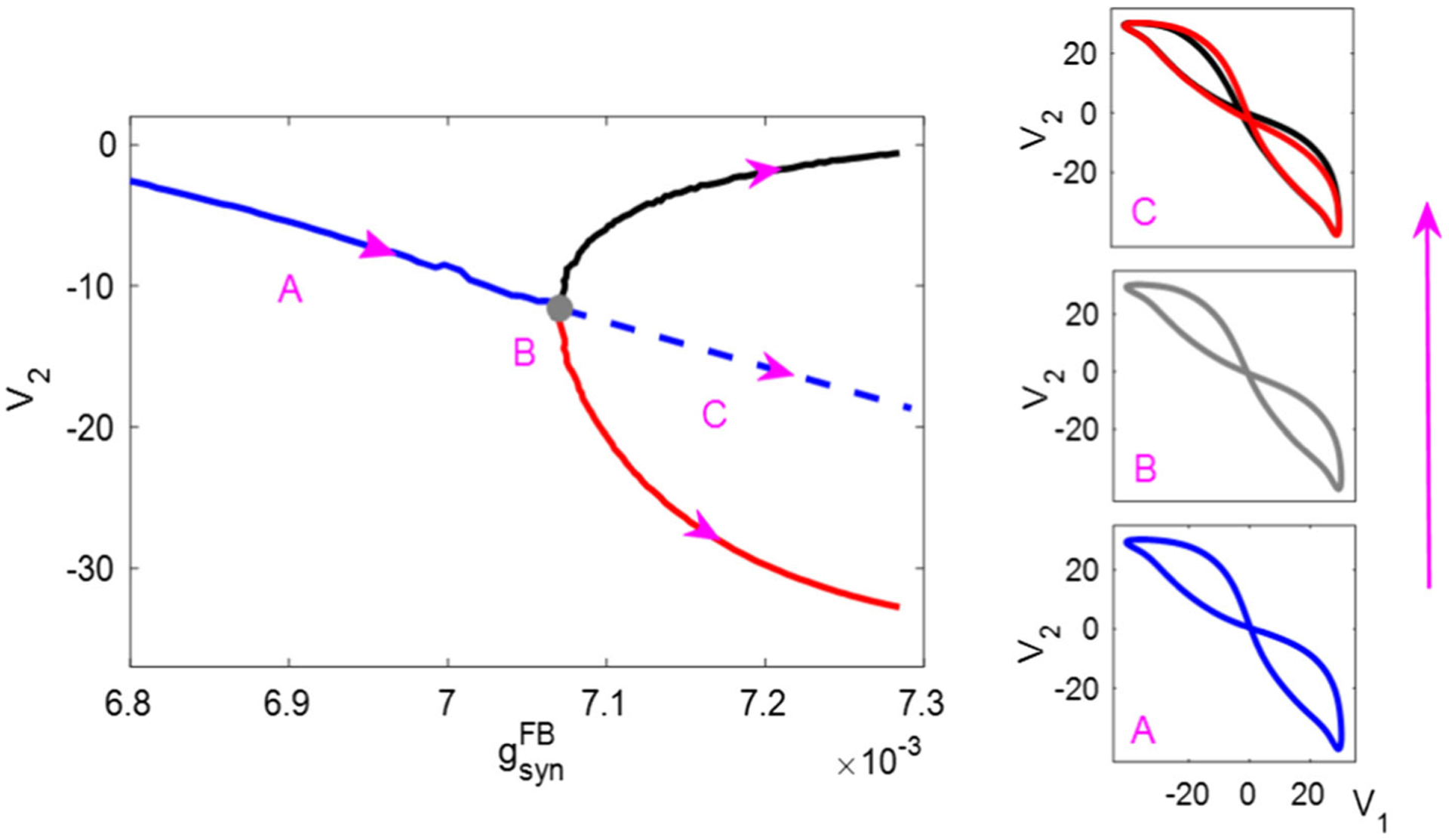
Supercritical pitchfork bifurcation on the middle band of the IR mechanism. Left: bifurcation diagram, recording the value of V₂ at the Poincaré section {V₁ = 20, dV₁/dt > 0} transverse to the limit cycle. Right: V₁ versus V₂ trajectory, occurring on region A (before bifurcation), B (on bifurcation) and C (after bifurcation) in the left panel. At $g_{\text{syn}}^{\text{CPG}}=0.008$, as $g_{\text{syn}}^{\text{FB}}$ increases to around 7.06×10⁻³ (gray point), two asymmetric stable limit cycles bifurcate from the symmetric stable one. Solid blue trace: symmetric stable limit cycles. Solid black/red trace: pairs of asymmetric stable limit cycles. Gray trace: limit cycle exactly on the bifurcation (dashed blue trace in the left diagram, representing a symmetric unstable solution, is extended by hand from the solid blue trace; available numerical methods do not allow its explicit identification, although its existence is indicated by the pitchfork bifurcation theorem for limit cycles [38])

Fig. 8.

Subcritical pitchfork bifurcation on the left border of the IR mechanism. Left: bifurcation diagram, recording the value of V₂ at the Poincaré section {V₁ = 20, dV₁/dt > 0} transverse to the limit cycle. Right: V₁ versus V₂ trajectory, occurring on region A (before bifurcation), B (on bifurcation) and C (after bifurcation) in the left panel. At $g_{\text{Syn}}^{\text{CPG}}=0.0016$, as $g_{\text{syn}}^{\text{FB}}$ passes 2.64 × 10⁻³ (gray point) from above, the stable limit cycle loses stability and an unstable limit cycle appears. Before bifurcation, there are two unstable limit cycle solutions coexisting with the stable one, consistent with a subcritical pitchfork. Solid blue trace: symmetric stable limit cycles. Dashed blue trace: symmetric unstable limit cycles. Dashed black/red trace: pairs of asymmetric unstable limit cycles. Gray trace: limit cycle exactly on the bifurcation

Table 1.

Detection of Fold vs Pitchfork Bifurcation

Mechanism	$g_{\text{syn}}^{\text{CPG}}$	$g_{\text{Syn}}^{\text{FB}}$	||Bv − v||	||Bv + v||	Type	Figures
Inhibition-release	0.008	0.00692	1.9934	0.0066	Pitchfork	Fig. 7
Inhibition-release	0.0016	0.002664	1.9916	0.0084	Pitchfork	Fig. 8
Inhibition-escape	0.0004	0.00355	1.9948	0.0052	Pitchfork	Fig. 15
Excitation-release	0.008	0.005565	0.0191	2.0191	Fold	Fig. 19

We then study the system’s robustness against disturbances (external perturbation) and measurement noise (internal noise) under different balances of the CPG conductance and FB conductance. To assess the response to external perturbation, we apply a 10% displacement away from the unperturbed periodic orbit at the maximal pendulum position in the trajectory, which results in an oscillatory behavior and convergence to the unperturbed limit cycle (see Fig. 9).

Fig. 9.

IR system ($g_{\text{syn}}^{\text{CPG}}=0.006$, $g_{\text{syn}}^{\text{FB}}=0.006$), initiated with a 10% displacement to the original maximal position, then allowed to converge back to the unperturbed trajectory

To describe this behavior, we compute the absolute percentage difference (error) between the minimal velocity of the perturbed and unperturbed trajectory, denoted by Δz in Fig. 9. Results are presented in Fig 10a.

Fig. 10.

Robustness of the IR mechanism against external and internal disturbances. a Under external perturbation, the absolute percentage difference (error) between the minimal velocity of the perturbed and unperturbed trajectory. b Under internal noise, the standard deviation of the maximal position of the noisy fluctuating trajectory over 100 periods

For every value of the CPG synaptic conductance, we observe that the larger the sensory feedback synaptic conductance is, the more quickly the perturbed trajectory returns to the unperturbed trajectory. The pure feedforward system $g_{\text{syn}}^{\text{FB}}=0$ shows the greatest error, consistent with Kuo’s observations.

However, the pure feedback system does not perform well when measurements of the system state are imperfect. We incorporate sensory pathway noise into the model as follows. We interpret the gating variable $S_{\infty }^{\text{FB}}$ in (18) as the open-state probability for a population of synaptic ion channels. To incorporate the noise arising from a finite population of channels, we replace the deterministic synaptic feedback current $-g_{\text{syn}}^{\text{FB}}{S}_{\infty }^{\text{FB}}\left(L_j\right)\left(V_i-E_{\text{syn}}^{\text{FB}}\right)$ with a fluctuating current represented by Gaussian white noise with the same mean and variance proportional to $S_{\infty }^{\text{FB}}\left(1-S_{\infty }^{\text{FB}}\right)$. That is, for each neuron cell i (≠ j), we replace (18) with

$$d{V}_i=\frac{1}{C}[I_{\text{ext}}-g_{\text{L}}\left(V_i-E_{\text{L}}\right)-g_{\text{Ca}}{M}_{\infty }\left(V_i\right)\left(V_i-E_{\text{Ca}}\right)-g_{\text{K}}{N}_i\left(V_i-E_{\text{K}}\right)-g_{\text{syn}}^{\text{CPG}}{S}_{\infty }^{\text{CPG}}\left(V_j\right)\left(V_i-E_{\text{syn}}^{\text{CPG}}\right)-g_{\text{syn}}^{\text{FB}}{S}_{\infty }^{\text{FB}}\left(L_j\right)\left(V_i-E_{\text{syn}}^{\text{FB}}\right)]dt+\frac{{ϵ}_{\text{FB}}}{C}{g}_{\text{syn}}^{\text{FB}}\left(V_i-E_{\text{syn}}^{\text{FB}}\right)\sqrt{S_{\infty }^{FB}\left(L_j\right)\left(1-S_{\infty }^{FB}\left(L_j\right)\right)}d{W}_i^{FB}(t).$$ (19)

Here, ϵ_FB, which is inversely proportional to the square root of the channel population size, controls the amount of noise in the sensory feedback channel. Of course, if $g_{\text{syn}}^{\text{FB}}$ is set to zero, then this source of noise vanishes trivially.

Such internal noise results in noisy fluctuating behavior of the pendulum (cf. Fig. 11). To quantitatively analyze this behavior, we compute the standard deviation of the maximal position of the noisy fluctuating trajectory each time the pendulum reaches the right extremum (z = 0) over 100 periods (see Fig. 10b). For every value of the CPG conductance, from Fig. 10b we observe that the dominant effect of increasing the FB conductance is to make the fluctuating trajectory deviate more relative to the deterministic limit cycle. The pure feedback system $g_{\text{syn}}^{\text{CPG}}=0$ shows much greater deviation than the pure feedforward system $g_{\text{syn}}^{\text{FB}}=0$, which is also consistent with Kuo’s observations.

Fig. 11.

IR system ($g_{\text{syn}}^{\text{CPG}}=0.006$, $g_{\text{syn}}^{\text{FB}}=0.006$) with internal noise in the feedback signal exhibits a noisy fluctuating behavior about the unperturbed trajectory over 100 periods

3.4. Inhibition-escape

Using the same method as Sect. 3.3, we compute the oscillation period and the second Floquet multiplier (see Fig. 12). For the range of the inhibition-escape mechanism, the main difference from that of the inhibition-release mechanism is that the pure CPG-feedforward system cannot generate periodic oscillations when the CPG’s synaptic conductance is large ($g_{\text{syn}}^{\text{CPG}}\gtrsim 1.0$, beyond the range shown). We use a nullcline structure to explain such inability to oscillate in Fig. 13. The increasing reciprocal inhibition from the active cell makes the inhibited cell rest at a voltage that is below the synaptic threshold, prohibiting its escape.

Fig. 12.

Oscillation period and the magnitude of the second Floquet multiplier of the inhibition-escape mechanism. a Period. b Next-to-largest magnitude Floquet multiplier

Fig. 13.

Phase portrait, V versus N, of the escape mechanism without feedback $\left(g_{\text{syn}}^{\text{FB}}\equiv 0\right)$, near the lower right boundary in Fig. 12. Two cube-shaped V-nullclines represent the active (red) and inhibited (blue) cells. The sigmoid-shaped N-nullcline (green) is identical for both active and inhibited cells. The synaptic threshold (magenta) is 0 mV. When the inihibition strength is small enough $\left(g_{\text{syn}}^{\text{CPG}}<0.0108\right)$, the intersection of N-nullcline and inhibited V-nullcline is on the middle branch (blue dot). Following the black trajectory, the inhibited cell reaches the left knee of its V-nullcline and jumps up to the active nullcline, inhibiting the other cell. When the inhibition strength grows above $g_{\text{syn}}^{\text{CPG}}=0.0108$, however, the inhibited nullcline becomes sufficiently lowered such that the intersection point lies on the left branch of the inihibited V-nullcline, prohibiting escape. This accounts for the disappearance of oscillations in the right bottom of Fig. 12

In Fig. 12b, when approaching the right boundary from above, an unstable limit cycle coexists with a stable fixed point (Fig. 14). As $g_{\text{syn}}^{\text{FB}}$ decreases, the unstable cycle shrinks to the stable fixed point via a subcritical Hopf bifurcation.

Fig. 14.

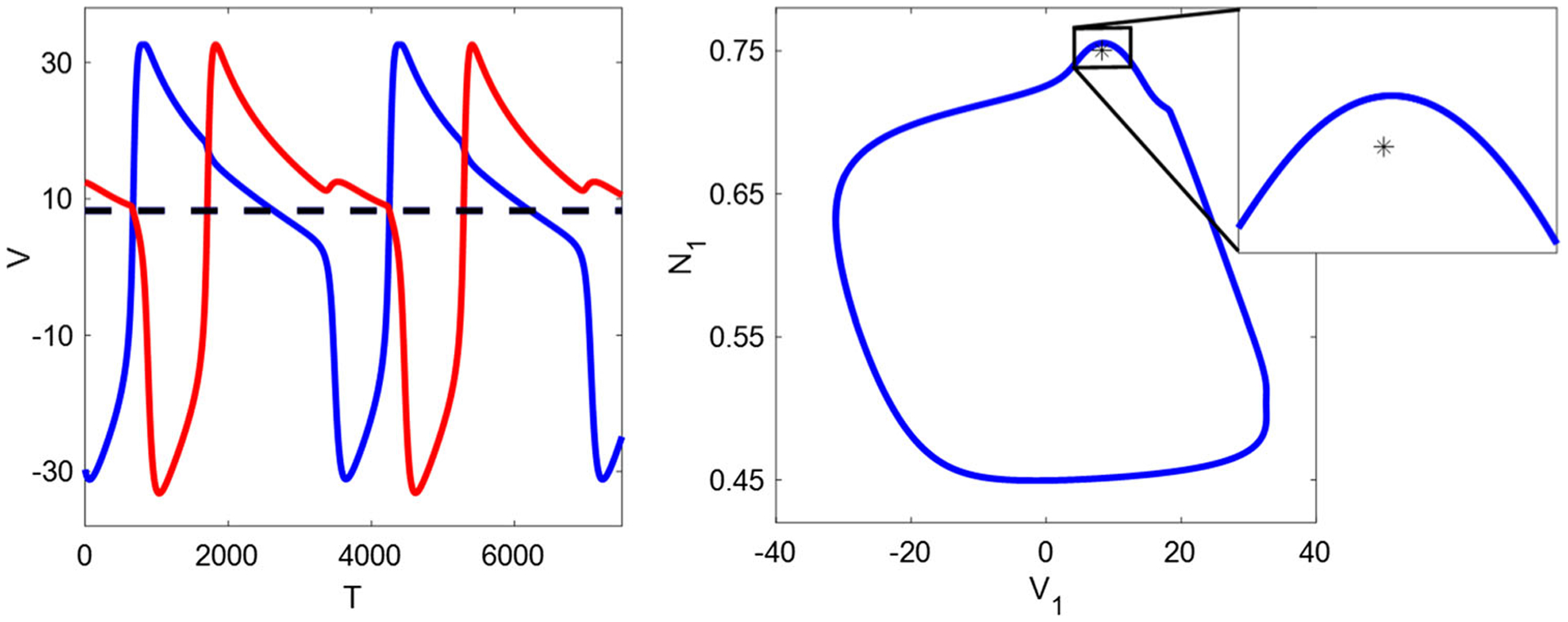
IE mechanism with $g_{\text{syn}}^{\text{CPG}}=0.012$ and $g_{\text{syn}}^{\text{FB}}=2.7145\times {10}^{-3}$, near the right domain boundary. A stable fixed point (black star) is surrounded by an unstable limit cycle (blue circle). The fixed point, with slowest decaying eigenvalue mode given by a complex conjugate pair with negative real part, coexists with the limit cycle, consistent with a subcritical Hopf bifurcation occurring on the boundary. Solid blue/red trace: cell 1/cell 2 on the unstable limit cycle. Dashed black/green trace: cell 1/cell 2 at the fixed point

Around the left border, there are two types of bifurcation. On the narrow black region close to the boundary, the unit-magnitude leading nontrivial Floquet multiplier implies a pitchfork-of-limit-cycle bifurcation, contributing to the generation of stable asymmetric limit cycles as described in Sect. 3.1. Figure 15 illustrates that as $g_{\text{syn}}^{\text{FB}}$ decreases, two stable nonsymmetric limit cycles, which are mirror images of each other, bifurcate from a stable one. See calculation results in Table 1 (p. 28). As the FB conductance further decreases, another bifurcation—subcritical Hopf bifurcation occurs exactly on the border, which results in the failure of oscillations in the parameter space. Figure 16 shows the coexistence of a stable fixed point and an asymmetric limit cycle when approaching to the bifurcatin point, as in the case shown in Fig. 14.

Fig. 15.

Supercritical pitchfork bifurcation near the left border of IE mechanism. Left: bifurcation diagram, recording the value of V₂ at the Poincaré section {V₁ = 20, dV₁/dt > 0} transverse to the limit cycle. Right: V₁ versus V₂ trajectory, occurring on region A (before bifurcation), B (on bifurcation) and C (after bifurcation) in the left panel. At $g_{\text{syn}}^{\text{CPG}}=0.0004$, as $g_{\text{syn}}^{\text{FB}}$ decreases to around 0.0035 (gray point), two asymmetric stable limit cycles bifurcate from the symmetric stable one. Colors as in Fig. 7

Fig. 16.

IE mechanism with $g_{\text{syn }}^{\text{CPG}}=0.0004$ and $g_{\text{syn}}^{\text{FB}}=2.35\times {10}^{-3}$, near the left boundary. A stable fixed point (black star) is surrounded by an unstable limit cycle (blue circle), consistent with a subcritical Hopf bifurcation occurring on the boundary. Solid blue/red trace: cell 1/cell 2 on the unstable limit cycle. Dashed black trace: cell 1/cell 2 with identical voltages at the fixed point

We quantify the robustness against external and internal disturbances in the inhibition-escape mechanism, with the same method as Sect. 3.3. The calculation results are shown in Fig. 17. Qualitatively, the larger the FB conductance, the more susceptible the system is to internal noise, and the more robust against external perturbation. Thus, this type of mechanism yields similar responses to noise as those of the inhibition-release mechanism (cf. Fig. 10), consistent with Kuo’s general conclusion.

Fig. 17.

Robustness of the IE mechanism against external and internal disturbances. a Under external perturbation, the absolute percentage difference (error) between the minimal velocity of the perturbed and unperturbed trajectory. b Under internal noise, the standard deviation of the maximal position of the noisy fluctuating trajectory over 100 periods

3.5. Excitation-release

A major difference between the inhibition-mediated mechanism and the excitation-mediated mechanism is that a purely feedback-driven system does not oscillate if the feedback is excitatory. Qualitatively, in the absence of the CPG or the feedback conductance, both cells sit in depolarization block, and some source of phasic inhibition is required to maintain rhythmic activity [57]. When the sensory feedback conductance is excitatory, we find that sensory feedback alone cannot sustain a periodic rhythm, and the (inhibitory) CPG conductance is required. Moreover, the larger the excitatory sensory feedback conductance, the more inhibitory the CPG conductance must be to sustain rhythmicity.

Like the inhibition-release system, the excitation-release system is unable to oscillate when the feedback conductance is large $\left(g_{\text{syn}}^{\text{FB}}\gtrsim 0.012\right)$. Figure 18 shows the shape of the (CPG, FB) range where periodic oscillations are observed, as well as the oscillation period and the magnitude of the second Floquet multiplier over the range.

Fig. 18.

Oscillation period and the magnitude of the second Floquet multiplier of the excitation-release mechanism. a Period. b Next-to-largest magnitude Floquet multiplier

In the excitation-release mechanism, there is only one type of bifurcation on its left boundary—a fold of limit cycles (see Fig. 19). A stable and an unstable limit cycles collide and annihilate each other on the boundary point. Descriptions of our bifurcation analysis and results are also detailed in Sect. 4.

Fig. 19.

Fold bifurcation on the left border of ER mechanism. Left: bifurcation diagram, recording the value of N₁ at the Poincaré section {V₁ = 20, dV₁/dt > 0} transverse to the limit cycle. Right: N₁ versus V₁ trajectory, occurring on region A (before bifurcation) and B (on bifurcation) in the left panel. At $g_{\text{syn}}^{\text{CPG}}=0.008$, as $g_{\text{syn}}^{\text{FB}}$ increases, a stable limit cycle (blue solid circle with the next-to-large magnitude Floquet multiplier smaller than 1) coexists with an unstable cycle (red dashed circle with the next-to-large magnitude Floquet multiplier larger than 1) until they coalesce at $g_{\text{syn}}^{\text{FB}}\approx 5.58\times {10}^{-3}$ (gray trace)

As in Sects. 3.3 and 3.4, Fig. 20 shows the system’s susceptibilities to the external perturbation and internal noise. Although the ER system is unable to support oscillations in the absence of feedforward signaling, its sensitivity to disturbances is consistent with Kuo’s system: for every value of the CPG conductance, as the FB conductance increases, the system grows increasingly robust against external perturbation but increasingly sensitive to internal noise.

Fig. 20.

Robustness of the ER mechanism against external and internal disturbances. a Under external perturbation, the absolute percentage difference (error) between the minimal velocity of the perturbed and unperturbed trajectory. b Under internal noise, the standard deviation of the maximal position of the noisy fluctuating trajectory over 100 periods

3.6. Excitation-escape

Like the inhibition-escape system (Fig. 12), the excitation-escape system in the absence of sensory feedback supports oscillations over a narrow range of CPG conductances $\left(0.0023\lesssim g_{\text{syn}}^{\text{CPG}}\lesssim 0.01\right)$. And like the excitation-release system (Fig. 18), increasing the excitatory sensory feedback conductance requires a compensating increase in the inhibitory CPG conductance. Consequently, we see a narrow band of (CPG, FB) conductances compatible with sustained oscillations. Thus, besides the inability to oscillate in a completely feedback-dependent system, the excitation-escape mechanism cannot sustain oscillation under a large CPG conductance and a small FB conductance—the range for the system to generate periodic oscillations is a narrow band. Moreover, the band narrows further as both conductances increase (not shown), although we have found sustained oscillations for, e.g., $g_{\text{syn}}^{\text{CPG}}=0.052$ and $g_{\text{syn}}^{\text{FB}}=0.057$. Figure 21 shows how the oscillation period and the magnitude of the leading nontrivial Floquet multiplier vary over the range of (CPG, FB) conductances for oscillations.

Fig. 21.

Oscillation period and the magnitude of the second Floquet multiplier of the excitation-escape mechanism. a Period. b Next-to-largest magnitude Floquet multiplier

At the left border of the excitation-escape mechanism, oscillations terminate in a torus bifurcation (see Fig. 22), which is a different mechanism from the bifurcation on the left boundary of the excitation-release mechanism. At the bifurcation point, there are two complex multipliers with (approximately) |μ| = 1 and one trivial multiplier with μ = 1. Following the bifurcation, we suspect the system develops an invariant torus. The properties of this torus are beyond the scope of the present paper. On the right boundary, the excitation-escape system bifurcates via a subcritical Hopf bifurcation and then loses the ability to oscillate. For instance, Fig. 23 shows the coexistence of a stable fixed point and an unstable limit cycle near the right border.

Fig. 22.

Torus bifurcation on the left border of EE mechanism. Left: bifurcation diagram, recording the value of N₁ at the Poincaré section {V₁ = 20, dV₁/dt > 0} transverse to the limit cycle. Right: N₁ versus V₁ trajectory, occurring on region A/B (before/on bifurcation) and C (after bifurcation) in the left panel. With $g_{\text{syn}}^{\text{CPG}}=0.008$, the system may develop an invariant torus at $g_{\text{syn}}^{\text{FB}}\approx 7.8\times {10}^{-3}$. Colors as in Fig. 19

Fig. 23.

EE mechanism with $g_{\text{syn}}^{\text{CPG}}=0.0132$ and $g_{\text{syn}}^{\text{FB}}=2.305\times {10}^{-3}$, near the right boundary. A stable fixed point (black star) is surrounded by an unstable limit cycle (blue circle). The fixed point, with seven negative-real-part eigenvalues, coexists with the limit cycle, consistent with a subcritical Hopf bifurcation occurring on the boundary. Solid blue/red trace: cell 1/cell 2 on the limit cycle. Dashed black/green trace: cell 1/cell 2 at the fixed point

Likewise, Fig. 24 shows how the system reacts to external and internal noise, which confirms Kuo’s outline as well as our observations in other three systems discussed above.

Fig. 24.

Robustness of the EE mechanism against external and internal disturbances. a Under external perturbation, the absolute percentage difference (error) between the minimal velocity of the perturbed and unperturbed trajectory. b Under internal noise, the standard deviation of the maximal position of the noisy fluctuating trajectory over 100 periods

4. Methods

4.1. Mathematical methods

Symmetry.

Limit cycle trajectories produced by the model fall in different symmetry classes. Eqs. (3), (13), (16), (18) define a dynamical system on $\Omega \subset {ℝ}^7$, dX/dt = F(X), with X = [V₁, V₂, N₁, N₂, A₁, A₂, x]^⊤ and F : $\Omega \to {ℝ}^7$ a smooth vector field. The model has a simple form of symmetry: exchanging the labels “1” and “2” and reversing the sign of x leaves the equations unchanged. Mathematically, we say that the dynamical system is equivariant with respect to the reflection group ${\mathbb{Z}}_2(\kappa )$ represented by the matrix

$${\mathcal{R}}_{\kappa }=\left(\begin{array}{ccccccc}& 1& & & & & \\ 1& & & 1& & & \\ & & 1& & & 1& \\ & & & & 1& & -1\\ & & & & & & \end{array}\right).$$ (20)

Equivariance means that for all X for which F is defined, $F\left({\mathcal{R}}_{\kappa }X\right)={\mathcal{R}}_{\kappa }F(X)$. Consequently, if X = ϕ (t) is a solution of $\dot{X}=F(X)$, then $Y={\mathcal{R}}_{\kappa }\varphi (t)$ is also a solution.

In a dynamical system with ${\mathbb{Z}}_2$ symmetry, we can also classify periodic orbits according to their symmetry. We observe two types of limit cycles occurring in our system: symmetric and nonsymmetric. In a symmetric solution, the solution and its mirror image are identical after a time delay of one half period. We make this statement precise with the following:

Definition 1 A T-periodic limit cycle solution X = γ (t) = γ (t + T) is symmetric if for all t ∈ [0, T), ${\mathcal{R}}_{\kappa }\gamma (t)=\gamma \left(t+T/2\right)$.

For a symmetric solution, the variables V, N, A of one unit coincide with those of the other unit half a period later, and the pendulum position is equal and opposite after half a period. Figure 3 shows an example of a symmetric solution.

To classify spontaneously occurring nonsymmetric behaviors, we adopt the following definition:

Definition 2 A T-periodic limit cycle solution X = γ (t) = γ (t + T) is asymmetric if ${\mathcal{R}}_{\kappa }\gamma (t)\ne \gamma (t+T/2)$.

Figure 4 shows an example. If X = γ₁(t) is an asymmetric limit cycle solution with period T, then $Y={\gamma }_2(t)={\mathcal{R}}_{\kappa }{\gamma }_1(t+T/2)$ is another, distinct solution.

Poincaré maps and bifurcations of limit cycles.

In order to study bifurcations of orbits as we vary the CPG and feedback conductance parameters, we define the Poincaré section

$${\Sigma }_1=\left\{V_1=0,\frac{d{V}_1}{dt}>0\right\}.$$ (21)

This section is transverse to the limit cycle at the point where the voltage of cell 1 crosses zero from below (cf. Figs. 3, 4). We also define a second section, Σ₂, which is the image of Σ₁ under the reflection operator:

$${\Sigma }_2={\mathcal{R}}_{\kappa }\left({\Sigma }_1\right)=\left\{V_2=0,\frac{d{V}_2}{dt}>0\right\}.$$ (22)

That is, Σ₂ is transverse to the limit cycle at the point where the voltage of cell 2 crosses zero from below. Let p₁ denote the point at which the limit cycle crosses Σ₁, and similarly p₂ ∈ Σ₂. For small displacements X₁ = p₁ + u₁ such that X₁ ∈ Σ₁ and |u₁| ≪ 1, we define the Poincaré map P₁ : Σ₁ → Σ₁ as the location in Σ₁ one cycle after starting from the displaced initial condition X₁. Following [38], §7.4 (Codimension 1 bifurcations of S-cycles), Lemma 7.6, we note that P₁ can be written P₁ = Q² for a smooth map Q : Σ₁ → Σ₁. Let B be the Jacobian matrix for Q at the fixed point p₁. At a bifurcation point where P₁ has a simple multiplier (eigenvalue) μ = 1 with eigenvector v, there are two scenarios: either Bv = v, in which case we have a fold-of-limit-cycle bifurcation; or else Bv = −v, in which case we have a pitchfork bifurcation.

4.2. Numerical methods

In order to identify the range of (CPG, FB) conductances that can sustain periodic oscillations, we sample initial conditions uniformly and at random from a compact subset of ${ℝ}^7$ containing a flow-invariant set Ω, namely V_i ∈ [V_max, V_min], N_i ∈ [0, 1], A_i ∈ [0, A_max], and x ∈ [−x_max, x_max] (see Appendix C). While this random sampling approach cannot exclude the coexistence of periodic orbits with stable fixed points, especially when (CPG, FB) lies on the boundaries of the range, it appears to yield consistent results, cf. Figs. 6, 12, 18, 21.

MatCont is a numerical tool for bifurcation analysis of parameterized dynamical systems [15]. Here, we exploit its ability to compute branches of codimension-1 bifurcations of equilibria and limit cycles and critical coefficients of periodic normal forms to a center manifold of the critical cycle. At an LPC-bifurcation, i.e., limit point (fold) bifurcation of cycles, where a limit cycle has a nonsemisimple Floquet multiplier μ = 1, MatCont computes the quadratic coefficient b of the normal form to the corresponding two-dimensional center manifold. When b ≠ 0, two limit cycles collide and disappear at the LPC point. See the example of LPC bifurcation in Fig. 19. At a PD bifurcation, i.e., period doubling (flip) bifurcation, where the limit cycle has a multiplier μ = −1, MatCont computes the cubic coefficient c of the normal form to the corresponding two-dimensional center manifold. If c ≠ 0, then a limit cycle of double the period bifurcates from the original limitcycle at the PD point; the new branch of limit cycles is stable if c < 0 and unstable if c > 0. At a NS bifurcation, i.e., Neimark–Sacker (torus) bifurcation, where the limit cycle has a pair of multipliers μ_1,2 = e^±iθ, 0 < θ < π, MatCont computes the real part of the cubic coefficient d of the normal form to the corresponding three-dimensional center manifold. If Re(d) ≠ 0, then an invariant torus bifurcates from the original limit cycle, stable within the center manifold if Re(d) < 0 and unstable if Re(d) > 0. See the example of NS bifurcation in Fig. 22.

In practice, around the bifurcation point detected in MatCont, which has a simple nontrivial Floquet multiplier μ = 1, we calculate the Jacobian matrix A = B² of the associated Poincaré map P₁ = Q². In order to calculate B, we apply to the point on section Σ₁ (cf. Eq. (21)) 1% displacement of the range in each of the 6 directions (V₂, N₁. N₂, A₁, A₂, x), respectively. We evolve a trajectory starting from Σ₁ until it crosses Σ₂ (cf. Eq. (22)) at point X₂, and then reflect $X_2\to {\mathcal{R}}_{\kappa }\left(X_2\right)$ to Σ₁. The six linear vectors on Σ₁ from the start point to the end point, divided by the respective displacement, form the 6×6 matrix B, and thus, the Jacobian matrix of P₁ is computed as B². At the point where P₁ has a simple eigenvalue μ = 1 with eigenvector v, there are two cases: either Bv = v (numerically 0 ≈ ∥Bv – v∥≪ ∥Bv – v∥), in which case we have a fold bifurcation (Fig. 19); or else Bv = −v (numerically 0 ≈ ∥Bv+v∥≪ ∥Bv−v∥), in which case we have a pitchfork bifurcation (Figs. 7, 8, 15). Table 1 presents the MATLAB calculation results. The parameter values (FB conductance) at the bifurcation point obtained with MATLAB agree with those produced by MatCont to within 1.4 × 10⁻⁴.

In addition to the bifurcation analysis, we also use MatCont to efficiently compute and record the oscillation period and Floquet multipliers (eigenvalues) in the process of the continuation of limit cycles (cf. Figs. 6, 12, 18, 21). Furthermore, we benefit from its ability to obtain unstable limit cycle solutions (cf. Figs. 8, 19, 22).

Simulation codes required to produce each figure and table are available at https://github.com/zhuojunyu-appliedmath/CPG-FB.

5. Discussion

Sensory feedback plays a significant role in the control of rhythmic movements. As one example, consider the regulation of breathing by circuits in the brainstem. The respiratory central pattern generator in the pre-Bötzinger complex can sustain fictive breathing in vitro [59] and may be modeled with an isolated single neuron [9] or a network of coupled respiratory neurons [10]. But in order to adapt to changes in metabolic load or changes in external metabolic gas concentrations (O2, CO2) the CPG has to be modulated by closed-loop sensory feedback [3–5,23,29,45,77]. As an illustration of Bässler’s principle, Diekman et al. showed that the eupneic (regular breathing) rhythm in the intact closed-loop pattern generator involves a dynamical mechanism distinct from the superficially similar rhythm generated by the open-loop central pattern generator [16], an effect that was consistent with experimental observations [17]. Similarly, sensory feedback changes the dynamical properties of the coupled brain–body–environment system in a closed-loop model for control of feeding movements in the marine mollusc Aplysia californica; in particular, sensory feedback was essential for maintaining robustness of swallowing despite resisting loads applied to food [40,56]. Sensory feedback can also change both the shape and timing of oscillation, which is particularly important when parts of the system operate on different timescales, e.g., the muscles developing force slowly compared to the switching times of neural elements [69].

For robotic locomotion control, the neural circuitry composed of coupled CPGs can produce rhythmic patterns of neural activity without rhythmic inputs [33]. In [61], Song has proposed that to generate steady and diverse human locomotion behaviours, reflex-based control (with no CPG) is functionally more important than central pattern generation; as supporting experimental evidence, the feedback-integrated model has similar response trends against disturbances as those of human walkers [62]. Similarly, a bipedal robotic controller, based on sensory reflexes and without any central pattern generators, can support stable robotic walking [44]. Song and Geyer showed that age-related declines in walking performance, including reduced walking economy and speed, resulted primarily from a loss of muscle strength and mass (as opposed to central nervous system deficits) [63]. This analysis of elderly walking further indicates the importance of sensory feedback relative to forward control.

Previous studies have considered the behavior of central pattern generator systems under parametric variation. For instance, [57] investigated mechanisms of frequency control in HCO systems and the sensitivity of the coupled oscillators’ period to synaptic thresholds. The adaptability of frequency (oscillation period) to alterations of excitatory drive depends strongly on the intrinsic neural mechanisms involved in rhythm generation. In particular, the CPG formed from units incorporating a slowly inactivating persistent sodium current (escape-type) achieves the greatest range of oscillation periods controlled by asymmetric external inputs [14]. To the best of our knowledge, previous studies of half-center oscillators (e.g., [14,57,68]) have not investigated the failure to maintain oscillations in the isolated CPG for large values of the CPG conductance, as we observe in the escape mechanism (Figs. 12 and 21, cf. horizontal axis where feedback conductance is zero.)

Kuo’s study [37] was abstracted from motor control systems for legged locomotion. As Kuo noted, the dynamics of the limbs contribute significantly to how they respond to descending motor commands. Thus, when sensory feedback is present, the limbs may be seen as oscillators that entrain the central circuit, in contrast to the usual interpretation in which the central circuit activity entrains the movement of the limbs. In the present study, we considered an overdamped muscle system closer to that of the feeding apparatus in the marine mollusc Aplysia californica, from which our muscle model was derived [75]. The half-center oscillator model we use to drive the biomechanical system is based on another invertebrate-derived system, the Morris–Lecar model. Here, rather than attempt to model a specific neuromechanical system, we follow Kuo in seeking general principles relating the relative roles of feedback and feedforward signals in a coupled brain–body model system. In contrast to Kuo’s model, we work in a continuous-time framework with a biologically derived muscle and HCO model.

Our results broadly confirm the observations made by Kuo.

First, we showed that it is possible to sustain oscillatory motor patterns in the intact system both with a purely feedforward system (with $g_{\text{Syn}}^{\text{FB}}$ set to zero) and with a purely feedback system (with $g_{\text{syn }}^{\text{CPG }}$ set to zero), as well as in mixed systems (both $g_{\text{syn}}^{\text{CPG}}>0$ and $g_{\text{syn}}^{\text{FB}}>0$). In our HCO framework, there are two distinct types of oscillation mechanisms at the level of the isolated HCO: escape and release [57,68]; we investigated parameters corresponding to both scenarios. Likewise, the topology of sensory feedback allows two distinct types: excitation-mediated and inhibition-mediated contralateral feedback. In our model, sensory feedback is contralateral, meaning feedback to CPG unit i is activated depending on the contraction or stretch state of muscle j ≠ i and is activated when muscle j is stretched. We could also consider ipsilateral feedback or feedback activated when the muscle is contracted rather than stretched. We found that each of these combinations behaves equivalently to a corresponding contralateral/stretch-activated version of the system, reducing the sixteen possible cases available a priori to the four functionally distinct cases we pursue in the paper. Taking into account these several possibilities, we showed that purely feedback-driven motor patterns, analogous to a chain reflex, occurred in the inhibition-mediated and not the excitation-mediated cases.

Second, we investigated the response of the system to external perturbation, and to internal noise. As Kuo argued, “The relative roles of feedforward and feedback should … be dependent on the relative significance of unexpected disturbances and imperfect sensors.” In Kuo’s discrete-time model, the purely feedforward system was susceptible to external disturbances, namely a 10% displacement of the initial velocity, whereas the system with feedback remained closer to the unperturbed trajectory under the perturbation. To pose a parallel question, we changed the initial position by making a 10% deviation away from the unperturbed orbit at a specific point in the trajectory, and measured the subsequent deviation in terms of the change in the minimum (greatest negative) velocity. For each fixed value of the CPG conductance, the relative absolute change in the minimal velocity shifted less and less, the greater the feedback conductance (Figs. 10a, 17a, 20a, 24a), consistent with Kuo’s observations. On the other hand, Kuo observed that purely feedback systems were susceptible to errors or noise in the measurement of the system state. We implemented “imperfect state measurements” by introducing a noisy synaptic feedback conductance. We found that the larger the FB conductance, the greater the position error, quantified as the spread of crossing points in a Poincaré section for the position at zero velocity (Figs. 10b, 17b, 20b, 24b). Once again, we confirmed Kuo’s fundamental observation.

By combining an explicit half-center oscillator circuit with a biomechanical model, we arrived at additional insights that reach beyond Kuo’s analysis.

Dependence of oscillation frequency on conductance parameters.

Prior investigations of half-center oscillators have studied the relationship between frequency of HCO cycling and parameters that could be subject to descending control or neuromodulation [14,57,58]. In [64,65], Spardy and colleagues observed the frequency increasing as a feedback conductance increased in a model for legged locomotion involving an escape-like CPG mechanism with excitatory sensory feedback. In our excitatory/escape configuration, cf. Fig. 21a, we also observe an increase in oscillator frequency (decrease in period) with increasing feedback conductance. We also observe decreasing frequency as the CPG conductance increases. For the excitation-release mechanism, we see frequency decreases with an increase in either the feedback or the synaptic conductance, consistent with [64]. In the inhibition-escape and inhibition-release scenarios, the period does not monotonically increase or decrease with feedback conductance, but shows a more complicated behavior.

Spontaneous symmetry breaking with sensory feedback.

We showed that incorporating sensory feedback allows the system to have a wider range of behaviors than the purely feedforward CPG-driven system, at least for the specific parameters used here. By construction, our CPG and biomechanical model has ${\mathbb{Z}}_2$ or mirror symmetry under exchange of the indices 1 ↔ 2 and reflection of the spatial axis x ↔ −x (see Sect. 3.1 and Sect. 4.1). This symmetry arises in many HCO-based CPG models as a mathematical idealization of the naturally occurring right/left symmetry found in bilateral organisms. Symmetric solutions are typical in such half-center oscillators. In such systems, a symmetric solution corresponds to a steady gait in which the animal moves forward without any bias toward the right or the left. Right/left nonsymmetric patterns of neuromotor activity can be induced to occur experimentally, either through a steering mechanism such as klinotaxis or chemotaxis in a swimming or crawling nematode [22,35], goal-driven steering in bioinsipred lamprey-like swimming robots [34,41], or through split-belt treadmill experiments that reproduce the effect of walking along a curved path [18,24]. In each of these examples, an external factor breaks the right/left symmetry: a gradient in salt concentration, a control signal set by a remote operator or uneven treadmill belt speeds. In contrast, spontaneous breaking of right/left CPG symmetry could provide a source for autopoietic steering behvior, which could play a role in escape from predation or random foraging behaviors.

Because we do not couple our model to an external substrate, we do not interpret its ${\mathbb{Z}}_2$ symmetry as a physical right/left symmetry, but rather as a purely mathematical property of the governing equations. Nevertheless, we can observe whether the solutions produced are symmetric or nonsymmetric. We find that in our model, for the parameter values considered in this paper, the pure feedforward system only exhibits symmetric movements (cf. Definition 1 on page 27), while combining feedforward and feedback control, in contrast, gives rise to both symmetric and nonsymmetric solutions (cf. Figs. 3, 4), the latter arising through supercritical pitchfork bifurcations (cf. Figs. 7, 15).

Although we do not observe nonsymmetric solutions in our system in the absence of sensory feedback, we point out that this observation does not reflect an underlying restriction imposed by the symmetry of our isolated HCO. Indeed, other systems with equivalent symmetry in the underlying equations have been shown to produce nonsymmetric solutions spontaneously without “sensory feedback.” For example, in a four-dimensional ${\mathbb{Z}}_2$-equivariant model constructed by coupling two identical Wilson–Cowan E–I oscillators, [6] observed a spontaneous symmetry-breaking bifurcation from a symmetric to a nonsymmetric limit cycle as a parameter was reduced (α₃, representing the strength of coupling from one excitatory population to the contralateral inhibitory population (cf. Fig. 7 of [6]).

Central pattern generators considered in isolation typically produce solutions with a discrete set of symmetries, cf. the discrete quadruped gaits discussed in [28]. In our system, when sensory feedback is included, we observe the emergence of nonsymmetric solutions ranging from nearly anti-phase (cf. Fig. 4) to nearly in phase. Figure 25 shows models with parameters $g_{\text{syn}}^{\text{FB}}=0.01$ fixed and $g_{\text{syn }}^{\text{CPG}}$ ranging from zero to 0.01, generating a continuum of nonsymmetric limit cycle solutions.

Fig. 25.

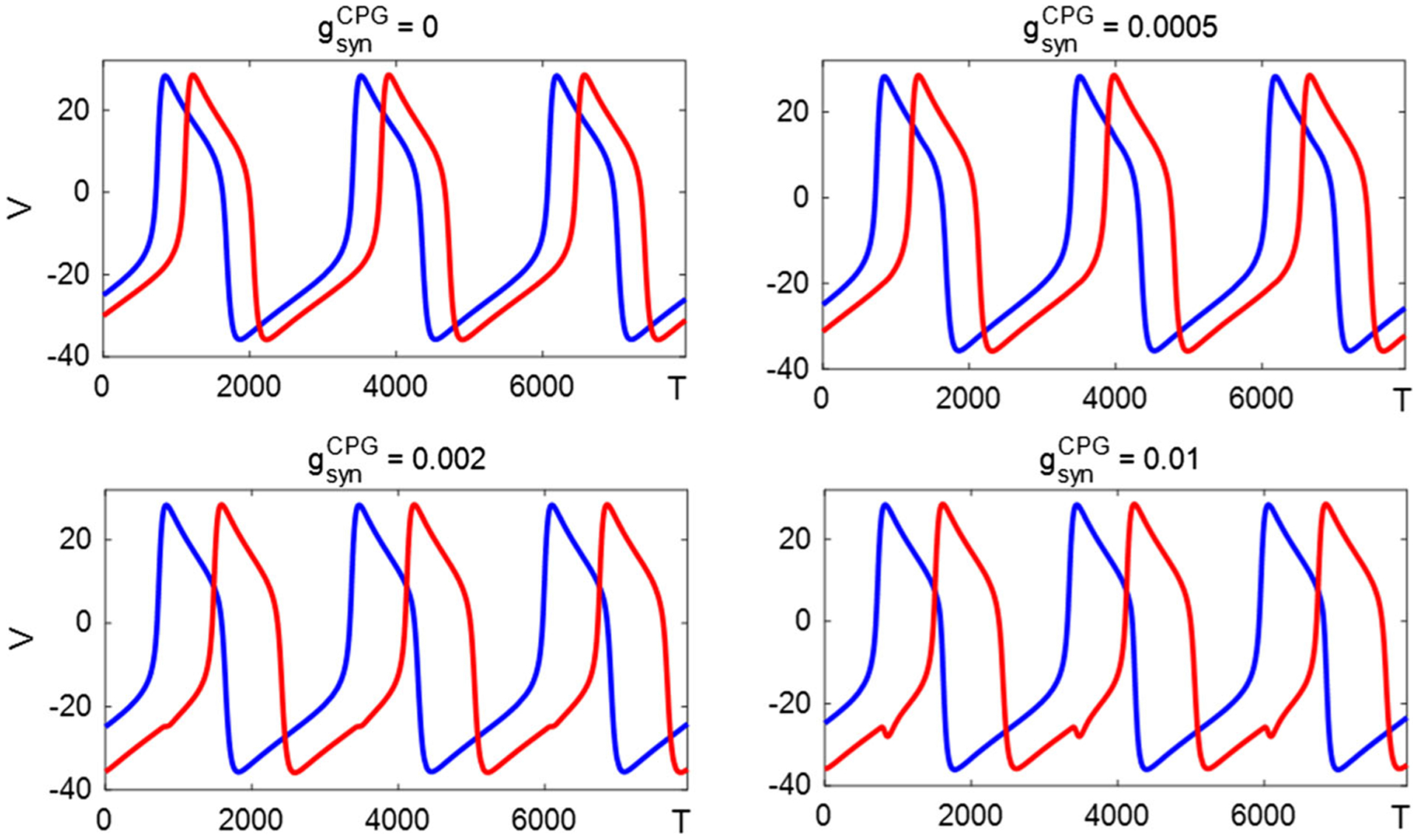
Inhibition-release system with sensory feedback can produce a continuum of nonsymmetric solutions, from nearly in-phase $\left(g_{\text{syn}}^{\text{CPG}}=0\right)$ to nearly anti-phase $\left(g_{\text{syn}}^{\text{CPG}}=0.01\right)$. V₁(t) (blue trace) is almost fixed and V₂(t) (red trace) shifts to the right

Escape and release.

Second, we find that the distinction between the escape and release mechanisms appears less stark in the presence of reciprocal CPG/biomechanical coupling, when internal noise is included in the sensory feedback pathway (cf. Fig. 26). When the rhythm is driven as much by the biomechanics as it is by the central activity, both inhibition-mediated escape and release systems have similar internal/external noise trade-offs (at least for the model and parameter values used here). Clearly, when the CPG conductance is set to zero, then “escape” and “release” are the same; if the CPG conductance is small, then the two cases remain similar (Fig. 27a). Likewise, if the feedback conductance is zero, then “inhibition” and “excitation” are the same; and they remain similar if the feedback is small (Fig. 27b).

Fig. 26.

Robustness to internal and external perturbations. In the two inhibition-mediated systems, the quantitative responses to external perturbation and internal noise fall on similar curves, indicating that the distinction between the release- and escape-mediated mechanisms is reduced in the presence of sensory feedback

Fig. 27.

Inhibition-dominated systems have similar internal/external noise trade-offs if the CPG conductance is small; release-mediated systems behave similarly if the FB conductance is small. a The absolute difference of the error caused by external perturbation between two inhibition-mediated systems. There is a slight difference if the conductance $g_{\text{syn }}^{\text{CPG }}$ is small. The range selected is the intersection of the two ranges in Figs. 10a and 17a. b Absolute difference of the error caused by internal noise between two release-mediated systems. The errors remain similar if $g_{\text{syn}}^{\text{FB}}$ is small. The range selected is the intersection of the two in Fig. 10b and 20b. For all parameter values examined, the absolute difference does not exceed 2%

These observations underscore our broad conclusion, that understanding mechanisms of robust motor control requires study not only of the isolated central pattern generator, but of the intact closed-loop system as a whole [2].

Limitations of our study and directions for future investigation.

As in any modeling study we restricted the scope of our investigation in several ways. For example, “robustness to external perturbations” could be interpreted in myriad ways; the definition of “robustness” is itself a matter of debate in theoretical biology (cf. discussion of this point in [40]). Here, we chose a specific measure of robustness intended to mirror the robustness measure used in [37]. Adopting a different measure of robustness to external perturbations would be expected to change our results quantitatively, but we expect our qualitative observations to remain similar.

In the same way, we implemented a specific measure of robustness to “internal noise.” Because extending Kuo’s analysis to a continuous-time biomechanical system was one motivation of this work, we chose an internal noise that aligned conceptually with Kuo’s “measurement noise” [37]. Since the only information about the state of the peripheral motor system available to the CPG is through the sensory feedback, it was natural to focus on the effects of noise in that pathway. Thus, in order to introduce noise in the feedback pathway, we replaced a deterministic synaptic feedback conductance with a fluctuating conductance based on a simple binomial noise model. While our model for synaptic noise is more realistic than, say, a generic white noise model of fixed variance, it nevertheless has an infinitely short correlation time, which is strictly speaking unrealistic for a real synapse. A more biophysically grounded noise model might introduce correlated noise or noise that reflects the underlying channel structure, cf. [1,53,71]. Noise could also be introduced naturally in other parts of the system besides the feedback conductance. For instance, we could include noise in the synaptic connection driving the CPG by replacing the term (6) in (18) with a term such as

$$\frac{{ϵ}_{\text{CPG}}}{C}{g}_{\text{syn}}^{\text{CPG}}\left(V_i-E_{\text{syn}}^{\text{CPG}}\right)\times \sqrt{S_{\infty }^{\text{CPG}}\left(V_j\right)\left(1-S_{\infty }^{\text{CPG}}\left(V_j\right)\right)}d{W}_i^{\text{CPG}}(t).$$

Similarly, we could include noise in the internal Morris–Lecar currents in the form

$$\frac{{ϵ}_{\text{K}}}{C}{g}_{\text{K}}\left(V_i-E_{\text{K}}\right)\sqrt{N_i\left(1-N_i\right)}d{W}_i^{\text{K}}(t),$$

$$\frac{{ϵ}_{\text{Ca}}}{C}{g}_{\text{Ca}}\left(V_i-E_{\text{Ca}}\right)\sqrt{M_{\infty }\left(V_i\right)\left(1-M_{\infty }\left(V_i\right)\right)}d{W}_i^{\text{Ca}}(t).$$

Each of these “internal” noise sources may impact the path and timing of the trajectory differently, depending on the balance of the FB and CPG conductances.

Although we base our biomechanical model on a specific example—the I2 muscle from the feeding apparatus of the marine mollusk Aplysia californica—our model is not intended as a detailed biomechanical model of that system. Decades of painstaking experimental work has developed detailed understanding of many aspects of the Aplysia feeding system neuromechanics [11,74], including kinematics [19,20,48–50], the role of mechanical reconfiguration and mechanical advantage of the grasper organ [51,67], the role of timing in ingestive vs. Egestive behaviors [47], the mechanical properties of the muscles and tissues involved [36,39,66], patterns of neural activity impinging on the I2 muscle during feeding behaviors [32] and measurements of the force produced by the feeding apparatus [26], and have led to a series of increasingly sophisticated computational models [40,56,70]. Despite these extensive prior studies, the detailed form of the sensory feedback from the muscles to the central circuitry remains unknown. In seeking to extend Kuo’s study [37] to a continuous-time model with realistic biomechanics, we chose the Aplysia I2 muscle because of the level of detail with which it has been described [75]. The known properties of the I2 muscle relevant for the present paper are its nonlinear length–tension curve (11), the dependence of muscle activation on neural input activity (12) and the muscle dynamics (13), which are slow relative to the neural dynamics. While the precise form of our biomechanics is specific to Aplysia and I2, the general properties are likely to be seen across many systems.

In the present study, we only explored the autonomous behavior of the system in the absence of sustained interactions with the outside world, that is, without considering the performance of some task. From a teleological point of view, the purpose of a central pattern generator is not merely to produce rhythmic activity, but rather to support a vital goal through interaction with the world external to the animal [12]. Examples of such brain–body–world systems include ingesting food against a resisting load [40,56], maintaining homeostasis against metabolic fluctuations [27], e.g., through breathing [16,17], regulation of blood pressure [73], locomotion across terrain [55] or through a viscous medium [13]. In such scenarios, the CPG/FB/biomechanical system typically will encounter sustained external perturbations, such as a load opposing motion in a particular direction. Together with a measure of “progress” (food consumed, calories burned, distance covered, body temperature maintained), these systems lead to interesting questions about the relative roles of FF and FB pathways in the pursuit of a more realistic goal than just maintaining a clocklike motor pattern. Whether differences in oscillation mechanism (escape/release, excitation/inhibition) have implications for function of a CPG when external loads are included remains an interesting, and important avenue for further study.

A. Table of Parameter Values

Table 2 specifies the parameter values used for simulations.

B. Model equations

For completeness, we list here the full equations of the model, as introduced in Sect. 2. The simulation codes are available from https://github.com/zhuojunyu-appliedmath/CPG-FB. Instructions for reproducing each figure and table in the paper are provided (see the README file at the github site).

For cell i (≠ j),

$$C\frac{d{V}_i}{dt}=I_{\text{ext}}-g_{\text{L}}\left(V_i-E_{\text{L}}\right)-g_{\text{Ca}}{M}_{\infty }\left(V_i\right)\left(V_i-E_{\text{Ca}}\right)-g_{\text{K}}{N}_i\left(V_i-E_{\text{K}}\right)-g_{\text{syn}}^{\text{CPG}}{S}_{\infty }^{\text{CPG}}\left(V_j\right)\left(V_i-E_{\text{syn}}^{\text{CPG}}\right)-g_{\text{syn}}^{\text{FB}}{S}_{\infty }^{\text{FB}}\left(L_j\right)\left(V_i-E_{\text{syn}}^{\text{FB}}\right),$$

$$\frac{d{N}_i}{dt}={\lambda }_N\left(V_i\right)\left(N_{\infty }\left(V_i\right)-N_i\right),$$

and

$$M_{\infty }\left(V_i\right)=\frac{1}{2}\left(1+\text{tanh}\left(\frac{V_i-E_1}{E_2}\right)\right),$$

$$N_{\infty }\left(V_i\right)=\frac{1}{2}\left(1+\text{tanh}\left(\frac{V_i-E_3}{E_4}\right)\right),$$

$${\lambda }_N\left(V_i\right)={\varphi }_N\left(\text{cosh}\left(\frac{V_i-E_3}{2E_4}\right)\right),$$

$$S_{\infty }^{\text{CPG}}\left(V_j\right)=\frac{1}{2}\left(1+\text{tanh}\left(\frac{V_j-E_{\text{thresh}}}{E_{\text{slope }}}\right)\right),$$

$$S_{\infty }^{\text{FB}}\left(L_j\right)=1-\frac{1}{2}\text{tanh}\left(\frac{L_j-x_0\ell }{L_{\text{slope}}}\right).$$

For muscle i,

$$F_i(t)=F_0\cdot a_i(t)\cdot LT\left(L_i(t)\right).$$

Here,

$$LT\left(L_i(t)\right)=-\left(5.27\times {10}^{-4}\right){\left(L_i(t)/\ell \right)}^2+0.1054\left(L_i(t)/\ell \right)-4.27,$$

$$L_i(t)=(50\pm 0.8x(t))\ell ,$$

$$L_j(t)=(50\mp 0.8x(t))\ell ,-50<x<50,$$

Table 2.

Parameter Values

Parameter	Value	Units	Parameter	Value	Units
C	1	μF/cm2	Ethresh	0 or 30	mV
Iext	0.8	μA/cm2	Eslope	2	mV
gL	0.005	μS/cm2	ϕN	0.0005	msec−1
gCa	0.015	μS/cm2	x0	0	None
gK	0.02	μS/cm2	ℓ	1	mm
EL	−50	mV	Lslope	200	mm
ECa	100	mV	τ	2.45	s
EK	−80	mV	F0	150	mN
$E_{\text{syn}}^{\text{CPG}}$	−80	mV	g	2	None
$E_{\text{syn}}^{\text{FB}}$	±80	mV	a0	0.165	None
El	0	mV	β	0.703	None
E2	15	mV	b	4×103	None
E3	0	mV	$g_{\text{syn}}^{\text{CPG}}$	as in Figure	μS/cm2
E4	15	mV	$g_{\text{syn}}^{\text{FB}}$	as in Figure	μS/cm2

and

$$a_i(t)=g\left[A_i(t)-a_0\right],0<a_i\le 1,$$

where

$$\begin{array}{rr}\hfill d{A}_i/dt=& \hfill {\tau }^{-1}\left\{U_i-\left[\beta +(1-\beta )U_i\right]A_i\right\},\\ \hfill U_i=& \hfill 1.03-4.31e^{\left(-0.198u_i\right)},0\le U_i\le 1,\\ \hfill u_i=& \hfill (1/2)V_i.\end{array}$$

The position of the pendulum is determined by

$$\frac{dx}{dt}=\frac{1}{b\ell }\left(F_2-F_1\right).$$

C. Flow-invariant set

Here we show that the state space of our system has a a compact flow-invariant domain, that is, a subset $\Omega \subset {ℝ}^7$ that is invariant under the flow generated by the model, forward in time. We describe the set as follows:

$$\left(V_1,V_2,N_1,N_2,A_1,A_2,x\right)\in \Omega ={\left[V_{\text{min}},V_{\text{max}}\right]}^2\times {[0,1]}^2\times {\left[0,A_{\text{max}}\right]}^2\times \left[-x_{\text{max}},x_{\text{max}}\right].$$ (23)

For the specific parameters, we use V_min ≈ −76.63 mV, V_max = 110 mV, A_max ≈ 1.021, and x_max ≈ 8.05.

For the range of N_i, since N_∞ ∈ [0, 1], N_i ∈ [0, 1] for all time as in Eq. (3). The voltage V_i ∈ [V_min, V_max] because if $V<V_{\text{min}},\frac{dV}{dt}>0$ for all values of the other variables’ ranges, and if $V>V_{\text{max}},\frac{dV}{dt}<0$ always holds. Considering the reversal potentials of all conductances, when V ≥ E_Ca, the maximal possible inward current would occur if the potassium, CPG and FB conductances were shut off $\left(N=0,S_{\infty }^{\text{CPG}}=S_{\infty }^{\text{FB}}=0\right)$, with extremal value of the calcium gate (M_∞) to be determined. Thus,

$$\frac{d{V}_i}{dt}\le I_{\text{ext}}-g_{\text{L}}\left(V_i-E_{\text{L}}\right)-g_{\text{Ca}}{M}_{\infty }\left(V_i-E_{\text{Ca}}\right)=\left(I_{\text{ext}}+g_{\text{L}}{E}_{\text{L}}+g_{\text{Ca}}{M}_{\infty }{E}_{\text{Ca}}\right)-\left(g_{\text{L}}+g_{\text{Ca}}{M}_{\infty }\right)V_i.$$

To make $\frac{d{V}_i}{dt}<0$ hold ∀ V_i > V_max, then,

$$\begin{gathered} V_{\text{max}}=\underset{M_{\infty }\in [0,1]}{\text{max}}\left\{\frac{I_{\text{ext}}+g_{\text{L}}{E}_{\text{L}}+g_{\text{Ca}}{M}_{\infty }{E}_{\text{Ca}}}{g_{\text{L}}+g_{\text{Ca}}{M}_{\infty }}\right\} \\ =\underset{M_{\infty }\in [0,1]}{\text{max}}\left\{\frac{I_{\text{ext}}+g_{\text{L}}{E}_{\text{L}}+E_{\text{Ca}}\left(g_{\text{L}}+g_{\text{Ca}}{M}_{\infty }\right)-E_{\text{Ca}}{g}_{\text{L}}}{g_{\text{L}}+g_{\text{Ca}}{M}_{\infty }}\right\} \\ =E_{\text{Ca}}+\underset{M_{\infty }\in [0,1]}{\text{max}}\left\{\frac{I_{\text{ext}}+g_{\text{L}}{E}_{\text{L}}-E_{\text{Ca}}{g}_{\text{L}}}{g_{\text{L}}+g_{\text{Ca}}{M}_{\infty }}\right\}. \end{gathered}$$

As M_∞ takes its minimum at 0, V_max = 110 mV for parameters we choose in Table 2.

In order to find V_min, we turn off the Ca²⁺ channel and allow for maximal inhibitory feedback:

$$\begin{gathered} \frac{d{V}_i}{dt}\ge I_{\text{ext}}-g_{\text{L}}\left(V_i-E_{\text{L}}\right)-g_{\text{K}}{N}_i\left(V_i-E_{\text{K}}\right)-g_{\text{syn}}^{\text{CPG}}{S}_{\infty }^{\text{CPG}}\left(V_i-E_{\text{syn}}^{\text{CPG}}\right)-g_{\text{syn}}^{\text{FB}}{S}_{\infty }^{\text{FB}}\left(V_i-E_{\text{syn}}^{\text{FB}}\right) \\ =\left(I_{\text{ext}}+g_{\text{L}}{E}_{\text{L}}+g_{\text{K}}{N}_i{E}_{\text{K}}+g_{\text{syn }}^{\text{CPG}}{S}_{\infty }^{\text{CPG}}{E}_{\text{syn}}^{\text{CPG}}+g_{\text{syn}}^{\text{FB}}{S}_{\infty }^{\text{FB}}{E}_{\text{syn}}^{\text{FB}}\right)-\left(g_{\text{L}}+g_{\text{K}}{N}_i+g_{\text{syn}}^{\text{CPG}}{S}_{\infty }^{\text{CPG}}+g_{\text{syn}}^{\text{FB}}{S}_{\infty }^{\text{FB}}\right)V_i. \end{gathered}$$

If $\frac{d{V}_i}{dt}>0$ always holds for arbitrary V_i < V_min, then

$$\begin{gathered} V_{\text{min}}=\underset{N_i,S_{\infty }^{\text{CPG}},S_{\infty }^{\text{FB}}\in [0,1]}{\text{min}}\left\{\frac{I_{\text{ext}}+g_{\text{L}}{E}_{\text{L}}+g_{\text{K}}{N}_i{E}_{\text{K}}+g_{\text{syn}}^{\text{CPG}}{S}_{\infty }^{\text{CPG}}{E}_{\text{syn}}^{\text{CPG}}+g_{\text{syn}}^{\text{FB}}{S}_{\infty }^{\text{FB}}{E}_{\text{syn}}^{\text{FB}}}{g_{\text{L}}+g_{\text{K}}{N}_i+g_{\text{syn}}^{\text{CPG}}{S}_{\infty }^{\text{CPG}}+g_{\text{syn}}^{\text{FB}}{S}_{\infty }^{\text{FB}}}\right\} \\ =\underset{N_i,S_{\infty }^{\text{CPG}},S_{\infty }^{\text{FB}}\in [0,1]}{\text{min}}\left\{\frac{I_{\text{ext}}+g_{\text{L}}{E}_{\text{L}}-80\left(g_{\text{L}}+g_{\text{K}}{N}_i+g_{\text{syn}}^{\text{CPG}}{S}_{\infty }^{\text{CPG}}+g_{\text{syn}}^{\text{FB}}{S}_{\infty }^{\text{FB}}\right)+80g_{\text{L}}}{g_{\text{L}}+g_{\text{K}}{N}_i+g_{\text{syn}}^{\text{CPG}}{S}_{\infty }^{\text{CPG}}+g_{\text{syn}}^{\text{FB}}{S}_{\infty }^{\text{FB}}}\right\} \\ =-80+\underset{N_i,S_{\infty }^{\text{CPG}},S_{\infty }^{\text{FB}}\in [0,1]}{\text{min}}\left\{\frac{I_{\text{ext}}+g_{\text{L}}{E}_{\text{L}}+80g_{\text{L}}}{g_{\text{L}}+g_{\text{K}}{N}_i+g_{\text{syn}}^{\text{CPG}}{S}_{\infty }^{\text{CPG}}+g_{\text{syn}}^{\text{FB}}{S}_{\infty }^{\text{FB}}}\right\}. \end{gathered}$$

When N_i, $S_{\infty }^{\text{CPG}}$ and $S_{\infty }^{\text{FB}}$ simultaneously reach their maximum, V_min ≈ −76.63 mV. For comparison, the voltage range in Fig. 2 roughly corresponds to V_min < V < V_max.

For the variables related to the biomechanics, as shown in Eq. (12), the range of U_i is

$$\left[0,U_{\text{max}}\right]=\left[0,f\left(V_{\text{max}}/2\right)\right]\subset [0,1.03).$$

The U-A relation, Eq. (13), gives

$$A_i\in \left[0,A_{\text{max}}\right]=\left[0,\frac{U_{\text{max}}}{\beta +(1-\beta )U_{\text{max}}}\right]\subset [0,1.021).$$

Since L₁ = (50 + 0.8x)ℓ and L₂ = (50 + 0.8x)ℓ, then as in Eq. (11),

$$LT\left(L_1\right)=-\left(5.27\times {10}^{-4}\right){(50+0.8x)}^2+0.1054(50+0.8x)-4.27,$$

$$LT\left(L_2\right)=-\left(5.27\times {10}^{-4}\right){(50-0.8x)}^2+0.1054(50-0.8x)-\mathrm{4.27.}$$

For convenience, we drop the length scale ℓ (= 1mm) since it does not affect the calculation result. Equation (14) defines the range for a_i: a_i ∈ (0, a_max] = (0, g(A_max − a₀)] ⊂ (0, 1.712). Because F_i is determined by a_i and x (Eq. (10)), and x is in turn determined by F_i (Eq. (16)), we can compute x_min and x_max through the ODE $dx/dt=\frac{1}{b}\left(F_2-F_1\right)$, i.e.,

$$\begin{gathered} \frac{dx}{dt}=\frac{1}{b}\left(F_2-F_1\right) \\ =\frac{1}{b}\left(F_0\cdot a_2\cdot LT\left(L_2\right)-F_0\cdot a_1\cdot LT\left(L_1\right)\right) \\ =\frac{F_0}{b}\left\{a_2\left[-\left(5.27\times {10}^{-4}\right){(50-0.8x)}^2+0.1054(50-0.8x)-4.27\right]-a_1\left[-\left(5.27\times {10}^{-4}\right){(50+0.8x)}^2+0.1054(50+0.8x)-4.27\right]\right\} \\ =\frac{F_0}{b}\left[\left(3.3728\times {10}^{-4}\right)\left(a_1-a_2\right)x^2-0.04216\left(a_1+a_2\right)x+0.3175\left(a_1-a_2\right)\right] \\ ≔\frac{F_0}{b}\left[W\left(a_1-a_2\right)x^2-Y\left(a_1-a_2\right)x+Z\left(a_1-a_2\right)\right]. \end{gathered}$$

On the one hand, if x > x_max, then $\frac{dx}{dt}<0$ for all other variables within their respective ranges. Thus, we aim to find x_max ∈ (−50, 50) such that for all x_max < x < 50, W(a₁ − a₂)x² −Y(a₁ + a₂)x + Z(a₁ − a₂) < 0 for arbitrary a₁, a₂ ∈ (0,1.712). If a₁ ≤ a₂, the inequality holds for all x > 0. When a₁ > a₂, x = 50 always satisfies the inequality, indicating that x_max(< 50) exists and should be the maximal abscissa of the left intersection of the quadratic function and horizontal axis, denoted by x_L:

$$\begin{gathered} x_L=\frac{Y\left(a_1+a_2\right)-\sqrt{Y^2{\left(a_1+a_2\right)}^2-4WZ{\left(a_1-a_2\right)}^2}}{2W\left(a_1-a_2\right)} \\ =\frac{Y}{2W}\left(\frac{1+\frac{a_2}{a_1}}{1-\frac{a_2}{a_1}}\right)-\frac{1}{2W}\sqrt{Y^2{\left(\frac{1+\frac{a_2}{a_1}}{1-\frac{a_2}{a_1}}\right)}^2-4WZ}. \end{gathered}$$

Let $t=\frac{a_2}{a_1}\in (0,1)$ and let $r=\frac{1+t}{1-t}=1+\frac{2}{\frac{1}{t}-1}$. Then r is a monotonically increasing function from 1 to ∞. Hence,

$$x_{\text{L}}=\frac{Y}{2W}r-\frac{1}{2W}\sqrt{Y^2{r}^2-4WZ}.$$

It is not hard to find that x_L monotonically decreases by calculating its derivative, and thus,

$$x_{\text{max}}={\left(x_L\right)}_{\text{max}}={x_L|}_{r=1}=\frac{Y-\sqrt{Y^2-4WZ}}{2W}\approx \mathrm{8.05.}$$

On the other hand, if x < x_min, then $\frac{dx}{dt}<0$ for all other variables within their respective ranges. Given the symmetry of our model, x_min = −x_max ≈ −8.05. Therefore, the flow-invariant set for the solutions of our HCO–muscle model has the form given by (23), with V_min ≈ −76.63 mV, V_max = 110 mV, A_max ≈ 1.021 and x_max ≈ 8.05 for the specific parameters used in this paper.

References

- 1.Anderson DF, Ermentrout B, Thomas PJ (2015) Stochastic representations of ion channel kinetics and exact stochastic simulation of neuronal dynamics. J Comput Neurosci 38(1):67–82 [DOI] [PubMed] [Google Scholar]
- 2.Bässler U (1986) On the definition of central pattern generator and its sensory control. Biol Cybern 54(1):65–69 [Google Scholar]
- 3.Ben-Tal A, Smith JC (2008) A model for control of breathing in mammals: coupling neural dynamics to peripheral gas exchange and transport. J Theor Biol 251(3):480–497 [DOI] [PMC free article] [PubMed] [Google Scholar]
- 4.Ben-Tal A, Tawhai MH (2013) Integrative approaches for modeling regulation and function of the respiratory system. Wiley Interdiscip Rev Syst Biol Med 5(6):687–699 [DOI] [PMC free article] [PubMed] [Google Scholar]
- 5.Ben-Tal A, Wang Y, Leite MCA (2019) The logic behind neural control of breathing pattern. Sci Rep 9(1):1–19 [DOI] [PMC free article] [PubMed] [Google Scholar]
- 6.Borisyuk GN, Borisyuk RM, Khibnik AI, Roose D (1995) Dynamics and bifurcations of two coupled neural oscillators with different connection types. Bull Math Biol 57(6):809–840 [DOI] [PubMed] [Google Scholar]
- 7.Brown TG (1914) On the nature of the fundamental activity of the nervous centres; together with an analysis of the conditioning of rhythmic activity in progression, and a theory of the evolution of function in the nervous system. J Physiol 48(1):18–46 [DOI] [PMC free article] [PubMed] [Google Scholar]
- 8.Brown TG (1911) The intrinsic factors in the act of progression in the mammal. Proc R Soc Lond Ser B 84(572):308–319 [Google Scholar]
- 9.Butera RJ Jr, Rinzel J, Smith JC (1999) Models of respiratory rhythm generation in the pre-Bötzinger complex I Bursting pacemaker neurons. J Neurophysiol 82(1):382–397 [DOI] [PubMed] [Google Scholar]
- 10.Butera RJ Jr, Rinzel J, Smith JC (1999) Models of respiratory rhythm generation in the pre-Bötzinger complex. II. Populations of coupled pacemaker neurons. J Neurophysiol 82(1):398–415 [DOI] [PubMed] [Google Scholar]
- 11.Chiel HJ (2007) Aplysia feeding biomechanics. Scholarpedia 2(9):4165 [Google Scholar]
- 12.Chiel HJ, Beer RD (1997) The brain has a body: adaptive behavior emerges from interactions of nervous system, body and environment. Trends Neurosci 20(12):553–557 [DOI] [PubMed] [Google Scholar]
- 13.Crespi A, Lachat D, Pasquier A, Ijspeert AJ (2008) Controlling swimming and crawling in a fish robot using a central pattern generator. Autonomous Robots 25(1–2):3–13 [Google Scholar]
- 14.Daun S, Rubin JE, Rybak IA (2009) Control of oscillation periods and phase durations in half-center central pattern generators: a comparative mechanistic analysis. J Comput Neurosci 27(1):3. [DOI] [PMC free article] [PubMed] [Google Scholar]
- 15.Dhooge A, Willy Govaerts YA, Kuznetsov HGEM, Sautois B (2008) New features of the software matcont for bifurcation analysis of dynamical systems. Math Comput Model Dyn Syst 14(2):147–175 [Google Scholar]
- 16.Diekman CO, Thomas PJ, Wilson CG (2017) Eupnea, tachypnea, and autoresuscitation in a closed-loop respiratory control model. J Neurophysiol 118(4):2194–2215 [DOI] [PMC free article] [PubMed] [Google Scholar]
- 17.Diekman CO, Thomas PJ, Wilson CG (2018) Experimental validation of a closed-loop respiratory control model using dynamic clamp. In: 2018 40th annual international conference of the IEEE engineering in medicine and biology society (EMBC). IEEE, pp 5273–5276 [DOI] [PubMed] [Google Scholar]
- 18.Dietz V, Zijlstra W, Duysens J (1994) Human neuronal interlimb coordination during split-belt locomotion. Exp Brain Res 101(3):513–520 [DOI] [PubMed] [Google Scholar]
- 19.Drushel RF, Neustadter DM, Hurwitz I, Crago PE, Chiel HJ (1998) Kinematic models of the buccal mass of Aplysia californica. J Exp Biol 201(10):1563–1583 [DOI] [PubMed] [Google Scholar]
- 20.Drushel RF, Sutton GP, Neustadter DM, Mangan EV, Adams BW, Crago PE, Chiel HJ (2002) Radula-centric and odontophore-centric kinematic models of swallowing in Aplysia californica. J Exp Biol 205(14):2029–2051 [DOI] [PubMed] [Google Scholar]
- 21.Ermentrout GB, Terman DH (2010) Mathematical foundations of neuroscience, vol 35. Springer, Berlin [Google Scholar]
- 22.Ferree TC, Lockery SR (1999) Computational rules for chemotaxis in the nematode C. elegans. J Comput Neurosci 6(3):263–277 [DOI] [PubMed] [Google Scholar]
- 23.Flor KC, Barnett WH, Karlen-Amarante M, Molkov Y, Zoccal DB (2019) Inhibitory control of active expiration by the bötzinger complex in rats. bioRxiv [DOI] [PMC free article] [PubMed] [Google Scholar]
- 24.Frigon A, Desrochers É, Thibaudier Y, Hurteau M-F, Dambreville C (2017) Left-right coordination from simple to extreme conditions during split-belt locomotion in the chronic spinal adult cat. J Physiol 595(1):341–361 [DOI] [PMC free article] [PubMed] [Google Scholar]
- 25.Gesslbauer B, Hruby LA, Roche AD, Farina D, Blumer R, Aszmann OC (2017) Axonal components of nerves innervating the human arm. Ann Neurol 82(3):396–408 [DOI] [PubMed] [Google Scholar]
- 26.Gill Jeffrey P, Chiel Hillel J (2020) Rapid adaptation to changing mechanical load by ordered recruitment of identified motor neurons. Eneuro. 10.1523/ENEURO.0016-20.2020 [DOI] [PMC free article] [PubMed] [Google Scholar]
- 27.Golubitsky M, Stewart I (2018) Homeostasis with multiple inputs. SIAM J Appl Dyn Syst 17(2):1816–1832 [Google Scholar]
- 28.Golubitsky M, Stewart I, Buono P-L, Collins JJ (1999) Symmetry in locomotor central pattern generators and animal gaits. Nature 401(6754):693–695 [DOI] [PubMed] [Google Scholar]
- 29.Grodins FS, June B, Bart AJ (1967) Mathematical analysis and digital simulation of the respiratory control system. J Appl Physiol 22(2):260–276 [DOI] [PubMed] [Google Scholar]
- 30.Guertin PA (2009) The mammalian central pattern generator for locomotion. Brain Res Rev 62(1):45–56 [DOI] [PubMed] [Google Scholar]
- 31.Harris-Warrick RM, Cohen AH (1985) Serotonin modulates the central pattern generator for locomotion in the isolated lamprey spinal cord. J Exp Biol 116(1):27–46 [DOI] [PubMed] [Google Scholar]
- 32.Hurwitz I, Neustadter D, Morton DW, Chiel HJ, Susswein AJ (1996) Activity patterns of the B31/B32 pattern initiators innervating the I2 muscle of the buccal mass during normal feeding movements in Aplysia californica. J Neurophysiol 75(4):1309–1326 [DOI] [PubMed] [Google Scholar]
- 33.Ijspeert AJ (2008) Central pattern generators for locomotion control in animals and robots: a review. Neural Netw 21(4):642–653 [DOI] [PubMed] [Google Scholar]
- 34.Ijspeert AJ, Crespi A (2007) Online trajectory generation in an amphibious snake robot using a lamprey-like central pattern generator model. In: Proceedings 2007 IEEE international conference on robotics and automation. IEEE, pp 262–268 [Google Scholar]
- 35.Izquierdo EJ, Beer RD (2013) Connecting a connectome to behavior: an ensemble of neuroanatomical models of C. elegans klinotaxis. PLoS Comput Biol 9(2):e1002890. [DOI] [PMC free article] [PubMed] [Google Scholar]
- 36.Kehl CE, Wu J, Lu S, Neustadter DM, Drushel RF, Smoldt RK, Chiel HJ (2019) Soft-surface grasping: radular opening in Aplysia californica. J Exp Biol 222(16):jeb191254. [DOI] [PMC free article] [PubMed] [Google Scholar]
- 37.Kuo AD (2002) The relative roles of feedforward and feedback in the control of rhythmic movements. Mot Control 6(2):129–145 [DOI] [PubMed] [Google Scholar]
- 38.Kuznetsov Y (2004) Elements of Applied Bifurcation Theory, vol 112. Springer, New York [Google Scholar]
- 39.Lu H, McManus JM, Cullins MJ, Chiel HJ (2015) Preparing the periphery for a subsequent behavior: motor neuronal activity during biting generates little force but prepares a retractor muscle to generate larger forces during swallowing in Aplysia. J Neurosci 35(12):5051–5066 [DOI] [PMC free article] [PubMed] [Google Scholar]
- 40.Lyttle DN, Gill JP, Shaw KM, Thomas PJ, Chiel HJ (2017) Robustness, flexibility, and sensitivity in a multifunctional motor control model. Biol Cybern 111(1):25–47 [DOI] [PMC free article] [PubMed] [Google Scholar]
- 41.Manfredi L, Assaf T, Mintchev S, Marrazza S, Capantini L, Orofino S, Ascari L, Grillner S, Wallén P, Ekeberg Ö et al. (2013) A bioinspired autonomous swimming robot as a tool for studying goal-directed locomotion. Biol Cybern 107(5):513–527 [DOI] [PubMed] [Google Scholar]
- 42.Maturana HR, Varela FJ (1980) Autopoiesis and cognition: The realization of the living, volume 42 of Boston Studies in the Philosophy of Science. D. Reidel Publishing Company, Boston [Google Scholar]
- 43.McManus Jeffrey M, Lu Hui, Chiel Hillel J (2012) An in vitro preparation for eliciting and recording feeding motor programs with physiological movements in Aplysia californica. JoVE 70:e4320. [DOI] [PMC free article] [PubMed] [Google Scholar]
- 44.Meng L, Macleod CA, Porr B, Gollee H (2018) Bipedal robotic walking control derived from analysis of human locomotion. Biol Cybern 112(3):277–290 [DOI] [PMC free article] [PubMed] [Google Scholar]
- 45.Molkov YI, Shevtsova NA, Park C, Ben-Tal A, Smith JC, Rubin JE, Rybak IA (2014) A closed-loop model of the respiratory system: focus on hypercapnia and active expiration. PloS one 9(10):e109894. [DOI] [PMC free article] [PubMed] [Google Scholar]
- 46.Morris C, Lecar H (1981) Voltage oscillations in the barnacle giant muscle fiber. Biophys J 35(1):193–213 [DOI] [PMC free article] [PubMed] [Google Scholar]
- 47.Morton DW, Chiel HJ (1993) The timing of activity in motor neurons that produce radula movements distinguishes ingestion from rejection in Aplysia. J Comp Physiol A 173(5):519–536 [DOI] [PubMed] [Google Scholar]
- 48.Neustadter DM, Drushel RF, Chiel HJ (2002) Kinematics of the buccal mass during swallowing based on magnetic resonance imaging in intact, behaving Aplysia californica. J Exp Biol 205(7):939–958 [DOI] [PubMed] [Google Scholar]
- 49.Neustadter DM, Drushel RF, Crago PE, Adams BW, Chiel HJ (2002) A kinematic model of swallowing in Aplysia californica based on radula/odontophore kinematics and in vivo magnetic resonance images. J Exp Biol 205(20):3177–3206 [DOI] [PubMed] [Google Scholar]
- 50.Neustadter David M, Herman Robert L, Drushel Richard F, Chestek David W, Chiel Hillel J (2007) The kinematics of multifunctionality: comparisons of biting and swallowing in Aplysia californica. J Exp Biol 210(2):238–260 [DOI] [PubMed] [Google Scholar]
- 51.Novakovic VA, Sutton GP, Neustadter DM, Beer RD, Chiel HJ (2006) Mechanical reconfiguration mediates swallowing and rejection in Aplysia californica. J Comp Physiol A 192(8):857. [DOI] [PubMed] [Google Scholar]
- 52.Pearson KG (1985) Are there central pattern generators for walking and flight in insects? In: Feedback and motor control in invertebrates and vertebrates. Springer, pp 307–315 [Google Scholar]
- 53.Pu Shusen, Thomas Peter J (2020) Fast and accurate langevin simulations of stochastic Hodgkin-Huxley dynamics. Neural Comput 32(10):1775–1835 [DOI] [PubMed] [Google Scholar]
- 54.Rinzel J, Ermentrout GB (1998) Analysis of neural excitability and oscillations. Methods Neuronal Model 2:251–292 [Google Scholar]
- 55.Schroer RT, Boggess MJ, Bachmann RJ, Quinn RD, Ritzmann RE (2004) Comparing cockroach and whegs robot body motions. In:IEEE International conference on robotics and automation, 2004. Proceedings. ICRA’04. 2004, vol 4. IEEE, pp 3288–3293 [Google Scholar]
- 56.Shaw Kendrick M, Lyttle David N, Gill Jeffrey P, Cullins Miranda J, McManus Jeffrey M, Hui L, Thomas Peter J, Chiel Hillel J (2015) The significance of dynamical architecture for adaptive responses to mechanical loads during rhythmic behavior. J Comput Neurosci 38(1):25–51 [DOI] [PMC free article] [PubMed] [Google Scholar]
- 57.Skinner FK, Kopell N, Marder E (1994) Mechanisms for oscillation and frequency control in reciprocally inhibitory model neural networks. J Comput Neurosci 1(1–2):69–87 [DOI] [PubMed] [Google Scholar]
- 58.Skinner FK, Turrigiano GG, Marder E (1993) Frequency and burst duration in oscillating neurons and two-cell networks. Biol Cybern 69(5–6):375–383 [PubMed] [Google Scholar]
- 59.Smith JC, Ellenberger HH, Ballanyi K, Richter DW, Feldman JL (1991) Pre-Botzinger complex: a brainstem region that may generate respiratory rhythm in mammals. Science 254(5032):726–729 [DOI] [PMC free article] [PubMed] [Google Scholar]
- 60.Somers D, Kopell N (1993) Rapid synchronization through fast threshold modulation. Biol Cybern 68(5):393–407 [DOI] [PubMed] [Google Scholar]
- 61.Song S, Geyer H (2015) A neural circuitry that emphasizes spinal feedback generates diverse behaviours of human locomotion. J Physiol 593(16):3493–3511 [DOI] [PMC free article] [PubMed] [Google Scholar]
- 62.Song S, Geyer H (2017) Evaluation of a neuromechanical walking control model using disturbance experiments. Frontiers Comput Neurosci 11:15. [DOI] [PMC free article] [PubMed] [Google Scholar]
- 63.Song S, Geyer H (2018) Predictive neuromechanical simulations indicate why walking performance declines with ageing. J Physiol 596(7):1199–1210 [DOI] [PMC free article] [PubMed] [Google Scholar]
- 64.Spardy LE, Markin SN, Shevtsova NA, Prilutsky BI, Rybak IA, Rubin JE (2011) A dynamical systems analysis of afferent control in a neuromechanical model of locomotion: I. Rhythm generation. J Neural Eng 8(6):065003. [DOI] [PMC free article] [PubMed] [Google Scholar]
- 65.Spardy LE, Markin SN, Shevtsova NA, Prilutsky BI, Rybak IA, Rubin JE (2011) A dynamical systems analysis of afferent control in a neuromechanical model of locomotion: II. Phase asymmetry. J Neural Eng 8(6):065004. [DOI] [PMC free article] [PubMed] [Google Scholar]
- 66.Sutton GP, Macknin JB, Gartman SS, Sunny GP, Beer RD, Crago PE, Neustadter DM, Chiel HJ (2004) Passive hinge forces in the feeding apparatus of Aplysia aid retraction during biting but not during swallowing. J Comp Physiol A 190(6):501–514 [DOI] [PubMed] [Google Scholar]
- 67.Sutton GP, Mangan EV, Neustadter DM, Beer RD, Crago PE, Chiel HJ (2004) Neural control exploits changing mechanical advantage and context dependence to generate different feeding responses in Aplysia. Biol Cybern 91(5):333–345 [DOI] [PubMed] [Google Scholar]
- 68.Wang X-J, Rinzel J (1992) Alternating and synchronous rhythms in reciprocally inhibitory model neurons. Neural Comput 4(1):84–97 [Google Scholar]
- 69.Wang Y, Gill JP, Chiel HJ, Thomas PJ (2021) Shape versus timing: linear responses of a limit cycle with hard boundaries under instantaneous and static perturbation. SIAM J Appl Dyn Syst (in press). arXiv preprint arXiv:1906.04387 [DOI] [PMC free article] [PubMed] [Google Scholar]
- 70.Webster-W VA, Gill JP, Thomas PJ, Chiel HJ (2020) Control for multifunctionality: Bioinspired control based on feeding in Aplysia californica. arXiv preprint arXiv:2008.04978 [DOI] [PMC free article] [PubMed] [Google Scholar]
- 71.White JA, Rubinstein JT, Kay AR (2000) Channel noise in neurons. Trends Neurosci 23(3):131–137 [DOI] [PubMed] [Google Scholar]
- 72.Norbert W (1948) Cybernetics or control and communication in the animal and the machine. Technology Press [Google Scholar]
- 73.Williams ND, Mehlsen J, Tran HT, Olufsen MS (2019) An optimal control approach for blood pressure regulation during head-up tilt. Biol Cybern 113(1–2):149–159 [DOI] [PMC free article] [PubMed] [Google Scholar]
- 74.Ye H, Morton DW, Chiel HJ (2006) Neuromechanics of multi-functionality during rejection in Aplysia californica. J Neurosci 26(42):10743–10755 [DOI] [PMC free article] [PubMed] [Google Scholar]
- 75.Yu Sung Nien, Crago PE, Chiel HJ (1999) Biomechanical properties and a kinetic simulation model of the smooth muscle I2 in the buccal mass of Aplysia. Biol Cybern 81(5–6):505–513 [DOI] [PubMed] [Google Scholar]
- 76.Zhang C, Lewis TJ (2013) Phase response properties of half-center oscillators. J Comput Neurosci 35(1):55–74 [DOI] [PubMed] [Google Scholar]
- 77.Zoccal DB, Silva JN, Barnett WH, Lemes EV, Falquetto B, Colombari E, Molkov YI, Moreira TS, Takakura AC (2018) Interaction between the retrotrapezoid nucleus and the parafacial respiratory group to regulate active expiration and sympathetic activity in rats. Am J Physiol Lung Cellular Mol Physiol 315(5):L891–L909 [DOI] [PMC free article] [PubMed] [Google Scholar]