

Abstract
We present a methodology for defining and optimizing a general force field for classical molecular simulations, and we describe its use to derive the Open Force Field 1.0.0 small molecule force field, code-named Parsley. Rather than traditional atom-typing, our approach builds on the SMIRKS-native Open Force Field (SMIRNOFF) parameter assignment formalism, which handles increases in the diversity and specificity of the force field definition without needlessly increasing the complexity of the specification. Parameters are optimized with the ForceBalance tool, based on reference quantum chemical data that include torsion potential energy profiles, optimized gas-phase structures, and vibrational frequencies. These quantum reference data are computed and are maintained with QCArchive, an open-source and freely available distributed computing and database software ecosystem. In this initial application of the method, we present essentially a full optimization of all valence parameters and report tests of the resulting force field against compounds and data types outside the training set. These tests show improvements in optimized geometries and conformational energetics and demonstrate that Parsley’s accuracy for liquid properties is similar to that of other general force fields, as is accuracy on binding free energies. We find that this initial Parsley force field affords accuracy similar to that of other general force fields when used to calculate relative binding free energies spanning 199 protein-ligand systems. Additionally, the resulting infrastructure allows us to rapidly optimize an entire new force field with minimal human intervention.
Graphical Abstract

1. Introduction
Molecular mechanics (MM) force fields are empirical models of molecular potential energy surfaces, which yield the potential energy and atomic forces as a function of the atomic positions. Force fields are a crucial component of molecular simulations in many domains of chemistry and biophysics. In particular, force fields are used in simulations of biomolecular systems that may include biopolymers, aqueous solvent, and small molecules such as metabolites and therapeutics. They are also fundamental to technologies used in computer-aided drug design, such as molecular docking1–7 and simulation-based calculations of protein-ligand binding free energies.8–15
Decades of work have led to relatively refined force fields for proteins made up of the 20 common amino acids.16–24 However, it is more difficult to develop a high quality general force field, i.e., one that applies to the wide range of small, organic molecules of interest in biology and drug discovery, due to the high diversity of the chemical space that must be considered. For example, the nearly 100 million compounds in the PubChem database25 embody many different combinations of varied functional groups and heterocycles. Moreover, some of the most important applications of force fields involve the simulation of as-yet undiscovered compounds, such as those under investigation for small molecule drug development, which may lie in new regions of chemical space. Small molecule force fields in wide use today include the general AMBER force field (GAFF),26 the CHARMM general force field (CGenFF),27 and the optimized potentials for liquid simulations force field (OPLS).28 These important tools have undergone continuous development, and current generations are applicable to a wide range of small molecules. Nonetheless, calculations of hydration free energies, partition coefficients, and other properties show that there is room for improvement in current general force fields.29–32 In addition, weaknesses in the small molecule component of the potential function likely account for some of the errors in calculations of noncovalent binding free energies relevant in host-guest chemistry33 and drug design.34
Improvements in force fields may come from the use of more and/or better reference data to optimize force field parameters, changes in the chemical typing rules used to assign parameters to atoms, and/or changes in the functional form of the force field. Exploring such improvements has traditionally involved considerable human input, and limitations in available computer power have made it difficult or impossible to carry out systematic explorations and optimizations. This has led to uncertainties in how exactly to go about attaining greater accuracy. For example, until it is clear how much accuracy can be achieved with a given functional form, it is impossible to ascertain whether or in what cases more accuracy is achieved by adding more detail and hence greater computational cost, e.g., by accounting explicitly for electronic polarizability. In addition, it is often unclear how the specific types and parameters of a given force field were arrived at, and this condition poses obstacles to reproducing and building on prior work. There is thus a need not only for improved force fields, but also for an infrastructure that will enable systematic exploration, optimization, and evaluation of new simulation force fields. Today, advances in software technology and increasing compute power make it possible to move toward the systematization and automation of force field generation.
The present study describes a significant step in this direction, the optimization of a small molecule force field using an automated and reproducible procedure, with all software, data, and workflows made freely available to the maximum extent possible. The result, OpenFF 1.0.0, code-named Parsley, is the first optimized force field using the SMIRNOFF format, with direct chemical perception.35 To create Parsley, we started with an initial force field called SMIRNOFF99Frosst consisting of direct chemical perception typing rules and parameters adopted from the Parm@Frosst force field.36 We then optimized nearly all 500 of the valence parameters to improve agreement with quantum chemical optimized geometries, energetics, and vibrational frequencies, while largely retaining the Lennard-Jones and electrostatic parameters of SMIRNOFF99Frosst. In keeping with the Open Force Field Initiative’s core philosophy, the Parsley force field and the software tools and data sets used to develop it are released under permissive open source licenses.
We also report here on the initial benchmarking of Parsley to show its improved accuracy relative to its predecessor for a wide variety of properties, especially energetics and geometries relative to gas phase quantum chemical calculations. The quantum chemical benchmarks, which cover more than 2,000 molecules and probe the quality of optimized geometries and relative conformer energies, show substantially better performance relative to SMIRNOFF99Frosst. For the condensed-phase properties, which span density, dielectric constant, heat of vaporization, excess molar volume, and enthalpy of mixing, no dramatic performance differences relative to SMIRNOFF99Frosst were noted in this release, and the overall accuracy is similar to that of GAFF; this was expected as nonbonded parameter optimization was not included as part of this work. In addition, as a reality check for the critical application area of computer-aided drug design, we report Parsley’s favorable performance in benchmark protein-ligand binding free energy calculations covering 199 protein-ligand pairs, along with comparative results for other small molecule force fields. Importantly, the infrastructure described here establishes a foundation for going far beyond Parsley, through the ongoing creation of a series of continually improving, open, small molecule force fields. The process reported here in the OpenFF 1.0.0 release continues in subsequent releases (OpenFF 1.1, 1.2 and 1.3)37–41 which will be described in follow-up work.
2. Methods
The infrastructure used to generate Parsley takes an initial force field as its starting point and optimizes it against reference training data to create an optimized force field, which in turn is benchmarked against test-set data prior to release (Figure 1). The software part of this infrastructure comprises a toolkit that assigns force field parameters to molecules of interest (openff toolkit); a component that computes a set of target properties for a set of input molecules (openff evaluator); and the ForceBalance code, which uses the openff evaluator to optimize force field parameters against the selected reference data. In general, the reference dataset can include both quantum chemical and experimental data. The Parsley force field was generated by refitting the parameters in the valence terms of the initial SMIRNOFF99Frosst35 force field against an extensive new set of high-level quantum mechanical data, which include energies, gas-phase geometries, and other properties. Note that the starting parameters in SMIRNOFF99Frosst in turn originated from two parent force fields, AMBER parm9942 and Merck’s parm@Frosst,36 which had been parameterized to reproduce gas phase geometries and energetics computed at lower levels of QM than that used here, for selected molecules. Here, Section 2.1 details the force field parameters that were optimized, the QM dataset used to drive the optimization, and the application of ForceBalance43 to carry out the optimization from the SMIRNOFF99Frosst35 starting point. Section 2.2 then describes how the resulting Parsley force field was tested against benchmark data outside the training sets, comprising gas phase properties from QM calculations, measured liquid-state properties, and measured protein-ligand binding free energies.
Figure 1.
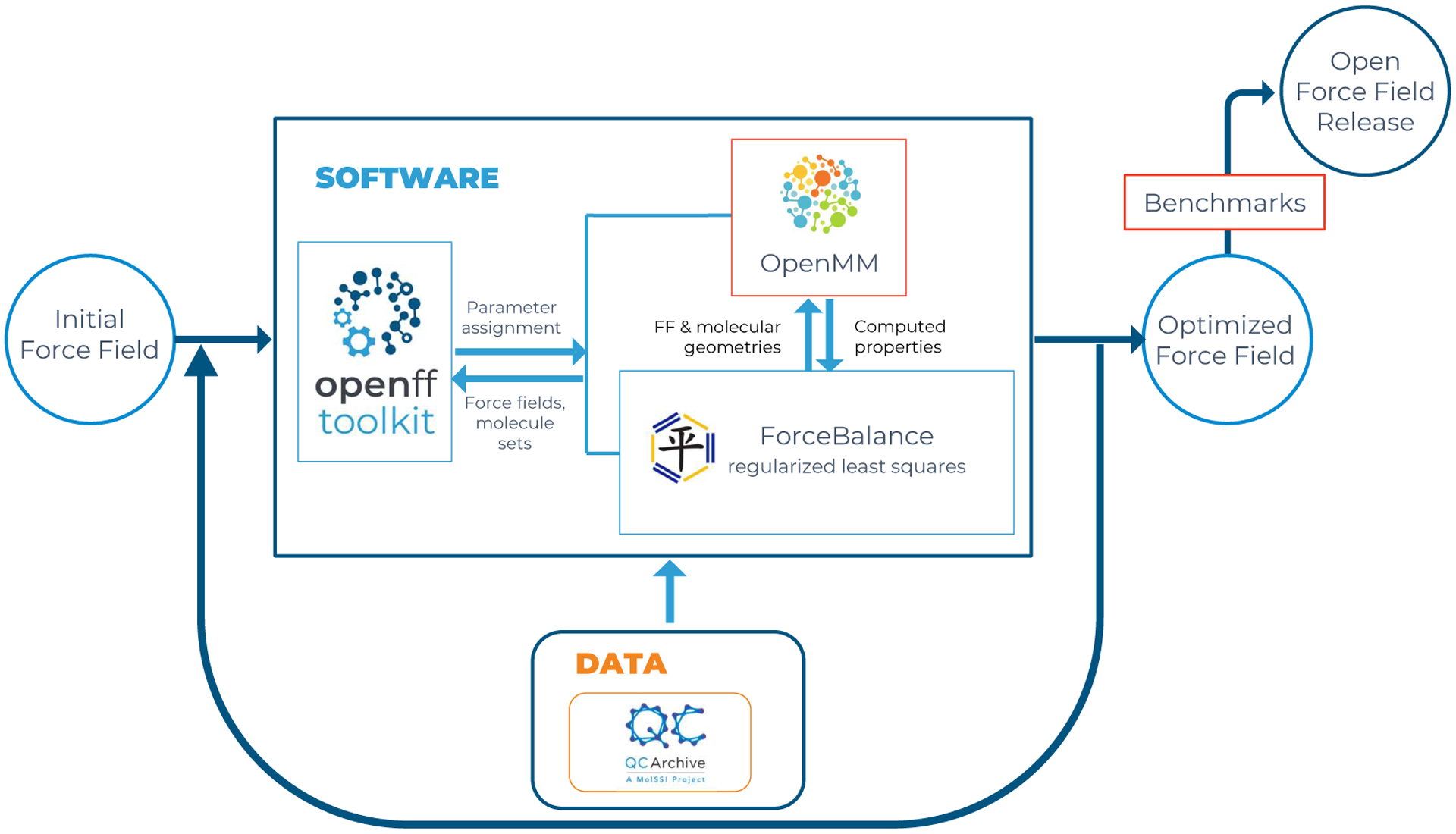
Open Force Field infrastructure and data flows during force field development. The OpenFF toolkit (left) sets up an MM simulation system from a given force field definition and parameters, and the OpenMM simulation code (top) is called to evaluate target physical properties. ForceBalance (middle) iteratively optimizes the parameters by least-squares minimization of an objective function constructed from the differences between MM simulated properties and reference data. QCArchive (bottom) is a distributed computing environment and database for generation and storage of quantum chemistry reference data. See text for further details.
2.1. Training the Parsley force field
2.1.1. Parameters that were refit
There are 500 valence parameters in SMIRNOFF99Frosst, and we aimed to optimize as many of these as possible. The quantum chemical data sets that we constructed 2.1.2 were successful at covering 481 of these parameters. The remaining 19 (Supporting Table S1), which were not modified due to the absence of training data (both in eMolecules, which we drew our coverage set from, and in our other available training data), either describe chemistries that are exceedingly rare in drug-like compounds or were superseded by other higher-priority parameters that matched the same chemical patterns.
All 481 parameters were fitted simultaneously against all QM data (Section 2.1.2). Each parameter definition is uniquely identified by an interaction type (e.g. bond stretch) and a SMIRKS pattern (e.g. [#6×4:1]-[#6×4:2]), and can contain one or more physical values (e.g. the bond length and the force constant). The full list of parameter definitions, which can be viewed in the published force field XML file, openff-1.0.0.offxml,44 may be summarized as follows:
Harmonic bond stretch: 86 equilibrium bond lengths and force constants.
Harmonic angle bend: 35 equilibrium angles and 39 force constants. These two numbers differ because four angles are linear and were kept linear during fitting.
Proper torsions: Each of the 154 torsion types is associated with an N-term Fourier series of potential energy contributions, where N ≤ 6, and each term, i, is of the form Ei = ki cos (iϕ + δi). We optimized all of the amplitudes that were defined in SMIRNOFF99Frosst, comprising 154, 62, 26, 5, 4 and 3 values of k1, k2, k3, k4, k5, and k6 respectively, for a total of 254 parameters. Parameters t156, t157, t158 represent torsion angles containing a linear angle, and their values of k1 were kept at 0.0 during fitting. The phase parameters, δi and the selection of Fourier terms used for each torsion were not optimized in this release.
Improper torsions: The four improper terms were kept unmodified, to avoid overfitting.
2.1.2. Compound sets used in training
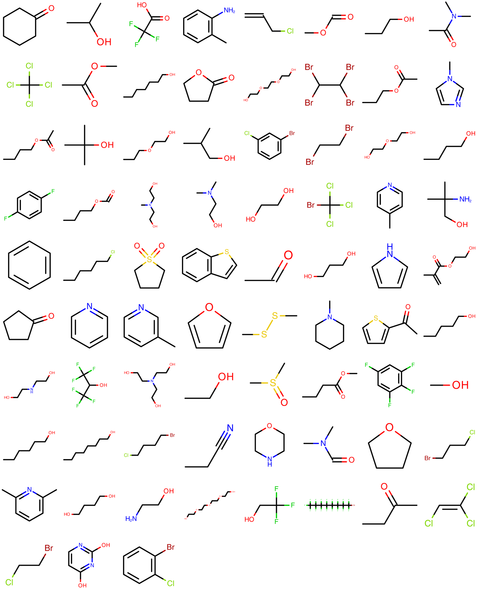
Two sets of small organic molecules were used to generate the quantum chemical datasets used in fitting. The first, termed the Roche Set, contains 468 fragment-sized molecules, most containing one to three rotatable bonds, that were provided by Roche as a collection of important and/or interesting chemistries. This data set was prepared using the MOE software.45 Representative compounds from this set are illustrated in Figure 2, and the full set can be found in Supporting Information section 1.1.2. The second, termed the Coverage Set, contains 80 molecules selected from eMolecules46 using a greedy algorithm aimed at providing parameter coverage for the maximum number of parameters using the minimum number of molecules. Figure 3 illustrates representative compounds, and a full list of SMILES can be found in Supporting Information section 1.1.2.
Figure 2.

An illustrative subset of small fragment-like molecules from the Roche Set.
Figure 3.

An illustrative subset of molecules from the Coverage Set.
Initial automated selection of the Coverage Set is described in a subdirectory of the openforcefields GitHub repository, and details of the additional molecules added manually to cover remaining gaps can be found in Supporting Information section 1.1.2.
2.1.3. Selection of quantum chemistry methodology
Quantum chemical calculations (geometry optimizations and torsion scans) were performed on a distributed set of high-performance computing clusters using the MolSSI QCFractal47 distributed quantum chemistry engine, with results deposited in the public MolSSI QCArchive Server (MQCAS)48,49 to allow open public access to all data. We used a single level of theory for all QM calculations, B3LYP-D3(BJ) / DZVP.50–53 This choice was based on two benchmark studies of conformational energies54,55 and our own initial studies that aimed to balance accuracy against computational cost. The molecules in both of these studies included amino acids, small to medium-sized peptides, and macrocycles. Geometries were optimized at the MP2/ccpVTZ level, and reference energies were computed using explicitly correlated focal point analysis methods considered to be equivalent to complete basis CCSD(T) in accuracy. Both studies found that B3LYP-D3(BJ) reproduces the reference energies with root-mean-squared errors (RMSEs) of < 1 kcal/mol when very large basis sets (e.g.def2-QZVP56) are used; the empirical D3 dispersion term played a major role, as the errors were typically 2–4x larger without it.
Notably, Řezáč et al. 201854 reported that the double-zeta quality DZVP basis set50 gave nearly the same RMSE as def2-QZVP, which we were able to reproduce in our own tests. When similar-sized and better-known basis sets such as 6-31G* and def2-SV(P) were used, the RMSEs increased significantly but there were only minor differences in computational cost. Our results are largely consistent with Řezáč et al. 201854 even though we did not use the custom empirical dispersion parameters they derived for the DZVP-DFT basis set. A scatter plot of RMSE vs. calculation time for a representative molecule, labeled as FGG114 in Řezáč et al. 2018.,54 is shown in Figure 4; the results confirm that the DZVP-DFT basis set gives the best compromise between accuracy and computational cost.
Figure 4. Tradeoff between speed and accuracy in selecting quantum chemical basis set.

Computational time (for single conformer) versus RMSE to benchmark-quality relative energies for 15 conformations of a representative molecule for several choices of basis set. The benchmark relative energies are MP2/CBS with a CCSD(T) correction and were obtained from Ref. 54.
Although we believe our choice of QM method is appropriate for gas-phase conformational energies for the neutral compounds comprising our training set here, we did not conduct benchmark studies on optimized geometries and vibrational frequencies which were also part of our parameterization dataset. We did not include charged molecules in the current training or test sets, because our use of QM gas-phase calculations as training data does not account for any differences in properties between gas phase and in aqueous solvent, which would be more pronounced in charged species. Therefore, the accuracy of this force field for charged species is presently unknown. This issue has been addressed in recent work on protein force fields in which the QM training data and MM calculations are both carried out in the presence of implicit solvent models,57 which may also be applicable to small molecule force fields. More comprehensive benchmarks are planned to inform future force field generations. However, the present level of theory is superior to the HF/6-31G* approach used in parameterizing the parm99/parm@Frosst force fields from which SMIRNOFF99Frosst descended, and thus should afford greater accuracy.
2.1.4. Generation of quantum chemical data for compound datasets
Prior to running quantum chemical calculations, the input molecules were subjected to protonation state and conformer expansion, using the Fragmenter software package.58 After the expansion, each protonation state was identified as a new molecule, so the number of distinct molecules increased; and each molecule could have one or more conformers. Each conformer provided one optimized geometry used in fitting. Three classes of gas phase quantum chemical data were generated for both the Roche and Coverage compound sets: optimized geometries, vibrational frequencies, and torsional energy profiles. The methods used are detailed below. The results of all quantum chemical calculations are stored as DataSet objects on the MQCAS48 and are freely available to the public. Examples of working with several MQCAS datasets can be found in Supporting Information section 1.1.3.
Optimized geometries
We used the MolSSI QCArchive Server (MQCAS) to store and distribute geometry optimizations with the geomeTRIC optimization driver59 and the Psi4 quantum chemistry package60,61 as backends. Optimized QM geometries were downloaded from the MQCAS, then filtered to remove cases where the bonding pattern changed on optimization, as well as issues which pose other problems for the openforcefield toolkit v0.4.1,62 e.g. undefined stereochemistry, missing torsion terms, or inability to assign AM1-BCC charges. Details can be found in Supporting Information section 1.1.3.
The objective function that measures deviations of MM from QM geometries is designed in the following way: MM geometry optimizations are first locally minimized starting from QM optimized structures, then MM and QM Cartesian coordinates are converted to lists of bond lengths, bond angles, and both proper and improper torsion angles. The difference between QM and MM optimized internal coordinates for a single molecule contributes to the objective function as:
| (1) |
where θ stands for the force field parameters used in the MM calculation, di refers to scaling factors of 0.05 Å, 8 degrees and 20 degrees for bond lengths, bond angles, and improper torsion angles, respectively. Proper torsion angles were not considered here, but instead are fitted based on comprehensive torsional energy profiles, as detailed below.
Vibrational frequencies
For each optimized geometry in the Roche and Coverage molecule sets, Hessian calculations were both executed and stored in the MQCAS. From the calculations that were completed, the Hessians for the lowest-energy conformation of each compound / protonation state were kept. After screening the dataset for topology changes and other errors, normal mode analysis was performed to obtain harmonic vibrational frequencies and Cartesian displacements for the internal degrees of freedom. Details can be found in Supporting Information section 1.1.3.
The corresponding force field Hessians were computed by locally minimizing the QM geometries with the force field, followed by evaluating forces with numerical displacements (0.001 Å). Normal mode analysis was carried out and the QM and FF frequencies were sorted from lowest to highest to yield the sorted sequences νQM,i and νFF,i, respectively. The objective function contribution for each set of normal modes was computed as the sum of squared differences of corresponding frequencies, scaled by a factor of dvib = 200cm−1, as:
| (2) |
Because the objective function sorts the QM and MM vibrational frequencies in simple ascending order, it does not account for possible differences between the QM and FF normal modes; i.e., the eigenvectors. This approach was taken primarily for computational efficiency, but it carries the risk of creating mismatches between the MM and QM vibrational modes. To test for this possibility, we also carried out single-point comparisons of vibrational frequencies where the MM frequencies and normal modes are permuted to maximize overlap with the QM normal modes. The permutation was carried out by computing the mass-weighted overlap matrix between each pair of QM and MM normal modes followed by solving the linear sum assignment problem. The objective function was then computed using the resulting matched pairs of QM and MM frequencies.
2.1.5. Torsional potentials
Quantum mechanical energy profiles were generated for dihedral angles in the Roche and Coverage sets. All calculations were carried out on the MQCAS, which employs the TorsionDrive software to compute each torsion energy profile using a wavefront propagation procedure,63 described briefly here. Multiple initial geometries were generated for each molecule via fragmenter and provided as input at the start of the procedure. Each input structure was energy-minimized with the selected torsion angle constrained to values on a 15° resolution grid, with QCArchive managing parallel job execution, and individual constrained optimizations handled by geomeTRIC/Psi4 as described above. At the conclusion of the constrained minimizations, the lowest-energy structure at each grid point was used to initiate new constrained minimizations at neighboring grid points. This cycle was repeated until the grid was fully populated with constrained minimization results and no new lowest-energy structures were found. In order to avoid pathologies such as bond-breaking that may occur when driving torsions into sterically hindered or high-energy regions, an upper energy limit was applied such that no constrained minimizations were started from structures with energies greater than 0.05 Hartrees (31.3 kcal/mol) above the minimum.
The set of lowest-energy constrained minimized structures for each grid point was downloaded from the MQCAS and checked for bonding topology changes; calculations that contained such changes were discarded. In addition, any scans that included a frame with an internal hydrogen bond were discarded to avoid having strong intramolecular nonbonded interactions in the gas-phase QM energy, as they would lower the accuracy of the fitted parameters for condensed phase simulations. Our work also suggests that including conformations with intramolecular hydrogen bonds can adversely affect torsion fitting by conflating the effects of strong internal electrostatic interactions (which might not be well described by point charge electrostatics, especially without simultaneous refitting) into fitted torsions. In future work, hydrogen-bonded dimers may be included along with intramolecularly hydrogen bonded conformers in order to assure a suitable balance, which implies a need to include fitting the nonbonded and valence parameters together.64 Hydrogen bonds were detected using the Baker Hubbard method (Angle(D-H..A) > 120 degrees and Dist(H..A) < 2.5 Å), as implemented in the MDTraj package.65 Details can be found in Supporting Information section 1.1.3.
For compounds in the Roche Set, torsional scans were generated for the 819 dihedral angles matching all of the following conditions:
the center bond is not part of a ring;
there is at least one heavy side group on both sides of the bond;
neither of the two angles involved is close to linear (≥ 165°).
Among all torsions sharing the same center bond, the one with the largest side groups, by number of atoms, was picked. For the compounds in the Coverage Set, we used the SMIRNOFF force field to label the torsions in each molecule and selected the first five dihedral angles that match each torsion term for scanning. (Note, however, that the force field term t155b was added after this dataset was created, so no torsion was selected for that term.)
The objective function contribution was computed as a weighted sum of squared differences between QM and MM energies. During the fitting process, each structure along the QM torsional profile was partially relaxed using the empirical force field being optimized. These MM optimizations were started from the QM constrained optimized structure, the four atoms defining the torsion were fixed at the QM coordinates, and all other atoms were held near the QM coordinates by applying harmonic energy restraints with force constant 1 kcal/mol/A2. These added harmonic restraints avoid the possibility of large structural changes of the MM structures away from the QM structures, which could make the torsional profile differences less meaningful. The restraint term is applied only in the MM energy minimization, and the MM energy at the energy-minimized geometry without the restraint term is used in subsequent steps. The QM and MM energies being compared were calculated as:
| (3) |
where the primes indicate absolute energies, subscripts indicate grid point indices, x0 is the lowest energy energy-minimized structure, θ represents the MM force field parameters, and OptMM(x; θ) denotes the MM constrained optimization procedure described above. The objective function is then calculated as:
| (4) |
where dE = 1.0 kcal mol−1 is a scaling factor. The weights are calculated by a formula that uses two cutoffs, where the weight is constant until the first cutoff (1.0 kcal/mol) then starts to decrease, followed by a hard second cutoff at 5.0 kcal/mol above which the weights are zero.
| (5) |
Our decisions regarding the fitting of torsion energy profiles warrant some discussion and comparison to published studies. Previously published force fields have either employed QM torsion scans similar to this work,66 or used custom MM simulations to generate input conformations for QM calculations.67 During the development of a nucleic acid force field, QM and MM minimizations were carried out prior to comparing energies in a similar procedure to this work.68 The weighting scheme we used is comparable with a previous study69 that employed a Boltzmann distribution with T = 2000 K (kBT ≈ 4.0 kcal/mol) to assign weights in fitting torsion energy profiles.
The variety of torsion fitting procedures used in prior studies shows that a standard procedure for carrying out this step is currently lacking. This is in part because each approach involves making a different set of compromises when fitting the approximate potential, and it is challenging to assess the impact of an approach on the accuracy of simulated properties. This and other challenges motivates the creation of automated benchmarking tools that are the subject of current research but beyond the scope of this paper.
2.1.6. Optimization algorithm and convergence criteria
The parameter optimization was carried out with ForceBalance,43 a Python toolkit to optimize force fields in a systematic, reproducible, scalable and flexible manner.43,70 We employed a development version of ForceBalance based on v1.6.071) to minimize the objective function. Support of the OpenFF force field was enabled by an interface with the OpenFF Toolkit v0.4.1.62 The commercial OpenEye toolkit version 2019.4.2 was used to generate .mol2 files, which are needed by ForceBalance to set up OpenFF simulations using the toolkit.
Numerical derivatives of the objective function with respect to parameters were computed with dimensionless displacements of 0.01 for improved numerical stability, relative to the ForceBalance default of 0.001. Fitting was terminated once two convergence criteria were met:
The dimensionless parameter step size fell below 0.01;
The objective function (Section 2.1.7) decreased by less than 0.1 during the step.
To efficiently optimize the parameters in as few iterations as possible, ForceBalance uses a quasi-Newton iteration to take near-optimal steps in parameter space:
To approximate the Hessian H(θ), ForceBalance computes an approximation to the matrix of second derivatives of each least-squares component in a manner that neglects parameter couplings:
| (6) |
The λ parameter is used to set the optimization step size, and was determined by line-search minimization for a given parametric gradient and Hessian. This strategy was employed because the line search over λ only requires repeated evaluation the objective function itself, and not the parametric gradient which is relatively expensive.
2.1.7. Objective function with regularization
ForceBalance was used to minimize an objective, or loss function, L(θ), with respect to force field parameters θ. The objective function quantifies deviation of quantities derived with the force field from the reference quantum chemical data while adding a regularization penalty to minimize the deviation from a reference set of parameters, following the standard approach for ForceBalance:43
Here, wi is the weight of each class of optimization data targets with corresponding loss functions Li(θ), which are often least-squares penalized loss:
where is an observed quantum chemical or physical property target to fit, and is the calculated value. wi of each target type was chosen to prevent the optimizer prioritizing one target type over other types. Carefully selected weights enabled the objective function contributions of different target types to have the same order of magnitude at the start of parameter optimization. Wreg is the regularization penalty weight, and Δθ quantifies the deviation from a reference set of parameters – here, the initial SMIRNOFF99Frosst v 1.1.0 parameter set.35 Regularization ensures that parameter adjustments are made conservatively to avoid introducing large problematic parameter changes that may only provide marginal improvements in the optimization target, especially when smaller datasets are used in parameterization. We used the regularization scales, σp listed in Table 2, based on past observations of variations in these parameter types in previous studies.70
Table 2.
Regularization scaling parameters used in ForceBalance optimization runs for each force field parameter type.
| parameter | regularization scale σp |
|---|---|
| bond force constant Kr | 100 kcal/mol/A2 |
| bond equilibrium length r0 | 0.1 Å |
| angle force constant Kθ | 100 kcal mol−1 rad2 |
| angle equilibrium angle θ0 | 20 degrees |
| proper torsion barrier height K | 1 kcal/mol |
| vdW well depth ϵ | 0.1 kcal/mol |
| vdW minimum rmin–half | 1 Å |
2.2. Testing the Parsley Force Field
Once the parameters had been trained as detailed in Section 2.1, we tested the resulting force field, Parsley-1.0.0, against optimized geometries outside the training set, and compared the results to those obtained with the initial force field, SMIRNOFF99Frosst-v1.1.0.35 We also tested Parsley against two data types outside the training set: energy differences among conformers of a given molecule, and physical properties of various organic liquids. Tests against vibrational spectra and torsional energy potentials are reserved for future studies. Benchmark comparisons of Parsley in the context of other general force fields are also available.72 We now describe how these tests were done.
2.2.1. Quantum chemical test set generation
The QCArchive tool was used to generate and archive additional QM data, using the procedures detailed in Section 2.1, for compounds in three collections.
OpenFF Discrepancy Benchmark 1 This comprises 2,802 fragment-like molecules (19,712 conformers) selected from the eMolecules catalog46 because their energy-minimized geometries are substantially different in SMIRNOFF99Frosst 1.0.8 relative to GAFF, GAFF2, MMFF94, and MMFF94s.73,74 We retained all protonation and tautomer states present in our initial dataset, but did not generate any additional ones. Further details can be found in Supporting Information section 1.2.1.
Pfizer Discrepancy Optimization Dataset 1 This comprises 100 fragment-like molecules for which Pfizer’s QM calculations of torsional profiles computed with HF/minix75 followed by B3LYP/6-31G*//B3LYP/6-31G** differed substantially from those generated with the OPLS3e force field. Pfizer code for relevant related work is public on GitHub.76 Enumeration of conformers, but not of protonation states, led to 352 conformers.
FDA Optimization Dataset 1 This is a subset of the list of FDA-approved drugs in the ZINC15 FDA dataset.77 Molecules were kept if they had 3–55 heavy atoms and consisted only of elements H, C, N, O, F, P, S, Cl, Br, I and B. We retained multiple protonation and tautomer states in the database, but did not generate any additional ones. Generation of up to 20 conformers per molecule led to 6,675 conformers for the 1,038 structures.
Test results are presented for the merger of these three datasets, termed the Full Benchmark Set. This dataset can be retrieved from the MQCAS as OpenFF Full Optimization Benchmark 1, as documented elsewhere.78 This is an “optimization dataset” in the sense that it – and the results presented here for benchmarking on this set – are for performance on optimized geometries only.
Conformational energy differences were assessed as follows. Compound conformers were energy-minimized using QM. For a compound with at least three conformers, we identified the conformer imin with the lowest QM energy and computed the energies of its other conformers relative to it: . We then computed the force field energies of the same conformers, Ei,FF , and, for each compound, computed the RMSE of from the corresponding QM energies. Note that conformation imin is based on the QM energies and used again for the FF energies.
2.2.2. Testing against physical properties of organic liquids
We assessed the ability of molecular dynamics simulations using the newly fitted Parsley force field to replicate 221 experimental observables for organic liquids spanning 104 molecules. The observables used are densities, heats of vaporization, and static dielectric constants, of pure liquids, and excess molar volumes and heats of mixing of binary liquid mixtures. The experimental data were drawn from the NIST ThermoML Archive.79 For systems involving water, the TIP3P model80 was used. Automated scripts used to select the data can be found in Supporting Information section 1.2.2.
We started with all available measurements of the properties listed above. When multiple values were available for a given quantity, only the ones with lowest reported uncertainties were retained. We furthermore excluded ionic liquids, compounds containing elements other than H, N, C, O, S, F, Cl, Br, and I, and data measured outside the temperature range 288–318K and the pressure range 0.95–1.05 atm. Dielectric constants < 10 were also excluded, because a force field that does not explicitly include electronic polarizability is not expected to replicate lower dielectric constants well.81 Finally, a greedy search was performed on the remaining data to select a minimal subset of small molecules that exercised the largest number of nonbonded parameter types and for which the most measurements were available. Sample compounds from the resulting set are shown in Figure 6, and further information on the data set can be found in Supporting Information section1.2.2.
Figure 6.
Representative molecules in the condensed phase physical property benchmark set.
Values for all of these properties were computed with the OpenFF-Evaluator (formerly named the PropertyEstimator) 0.0.5 tool, using scripts which can be found in Supporting Information section1.2.2. Calculations were carried out with the new Parsley 1.0.0, and, for comparison, with its precursor, SMIRNOFF99frosst 1.1.0, as well as GAFF 1.81 and GAFF 2.11.
2.2.3. Testing against protein-ligand binding free energies
We assessed the performance of the newly fitted Parsley forcefield in binding free energy calculations based on molecular dynamics simulations following suggested best practices for benchmarking binding affinities.82 The test set consisted of 8 protein targets with a total of 199 ligands (Supporting Information, Table 2), using a set commonly referred to as the “JACS dataset” from a prior study published in that journal and frequently used by the community.12 For a fair comparison to previously published results, the initial ligand and protein structures were obtained from prior benchmark work.83 These structures are available in the protein-ligand-benchmark repository.84 Relative binding free energies were calculated employing alchemical perturbations between pairs of ligands in water and the protein complex. These calculations employed a non-equilibrium workflow based on GROMACS and pmx.85,86 For the ligand molecules, the Parsley force-field was used as parameters. The protein was parameterized with the AMBER ff99sb*ILDN force field87–89 and a TIP3P explicit water model was employed. We chose AMBER ff99sb*ILDN as the protein force field because we expect Parsley to have the best compatibility with the AMBER family of force fields, as its non-bonded parameters are ultimately taken from Parm@Frosst, an AMBER-compatible small molecule force field.36 The water model was chosen as TIP3P due to the widespread use of this water model with the AMBER family of protein force fields. To mimic physiological conditions, ions (150 mM NaCl) and additional counterions to neutralize the system were added to the dodecahedral simulation boxes.
The analysis workflow used for analyzing the calculations is available in 90. The statistics in this workflow were calculated using Arsenic,91 which is a package implementing best practices for consistently calculating statistics and reporting results from binding free energy calculations. The Parsley results were compared to previously published results using the GAFF2.1,26 CGenFF3.0.127 and OPLS3e34,66 force fields. The former GAFF2.1 and CGenFF results were calculated with the same pmx worklow, and the OPLS3e results were calculated with Schrödinger FEP+.83
More detailed discussion of the workflow, the employed parameters and the analysis can be found in the Supporting Information. Full details of this study will be reported in a forthcoming publication, and a preliminary report can be found in 92.
3. Results and Discussion
This section first describes the consequences of parameter optimization for accuracy over the training set, and then benchmarks Parsley on the separate test set compounds and properties. The test set results should be indicative of Parsley’s accuracy in new applications.
3.1. Improvements in accuracy over training set data
3.1.1. Optimization of the objective function
The parameter fitting process dramatically increased the accuracy of the force field for the training data. Although this was anticipated, it is important to confirm, because it verifies the effectiveness of the optimization procedures and provides a scale for the degree of improvement. The dimensionless objective (or loss) function—the weighted sum of squared differences between QM and MM values—decreased dramatically in the fitting, from 25,708 to 4,522 (Figure 7). As described in Section 2.1, the objective function is a sum of contributions which report the accuracy of optimized geometries, vibrational spectra, and torsional energy profiles. The effect of training on these components is summarized in Table 3 (Training Set data) and Figure 8, and the following subsections provide further details of these results. Full fitting details, as well as inputs and outputs, can be found in the release package.93
Figure 7.

Objective function, or loss function, plotted against the number of ForceBalance iterations.
Table 3.
Overall change in root-mean-squared error (RMSE) metrics vs. the quantum chemical result calculated for four types of properties, using the initial and optimized force field, and divided into training set and test set. The numbers in parentheses under vibrational spectra indicate RMSE in frequencies after permutation of MM normal modes to maximize overlap with QM normal modes. ND = No Data.
| Training set | Full test set | ||||||
|---|---|---|---|---|---|---|---|
| Data class | Initial RMSE | Final RMSE | Change (%) | Initial RMSE | Final RMSE | Change (%) | |
|
Geometry
optimization |
Bond lengths
(Å) |
0.045 | 0.023 | −49% | 0.023 | 0.017 | −33% |
|
Bond angles
(deg) |
3.71 | 3.20 | −14% | 3.80 | 3.59 | −5.5% | |
|
Improper
dihedrals (deg) |
4.15 | 2.87 | −31% | 4.31 | 2.82 | −35% | |
| Vibrational spectra (with mode reassignment) |
Frequencies
(cm−1) |
119. (156.) |
39.6 (90.) |
−67% (−42%) |
ND | ND | ND |
| Torsion energy profiles |
Energies
(kcal/mol) |
2.96 | 1.89 | −36% | ND | ND | ND |
|
Relative
energies |
Energies
(kcal/mol) |
ND | ND | ND | 2.43 | 2.13 | −12% |
Figure 8. Improvement in components of the training set and test set objective functions with fitting.

Red histogram shows performance with our initial force field, green histogram shows performance with the optimized force field and blue histogram shows the distribution of changes in objective function contribution of each target (individual molecules/geometries contributing to the objective function) due to the parameter optimization. Left column (a–c) provides the training set results. Right column (d–e) provides test set results. The range of each plot encompasses ≥ 94.94 % of the population of initial objective function contributions and ≥ 99.2 % of the population of final objective function contributions.
3.1.2. Optimized geometries
The geometric component of the objective function is computed from the deviations of bond-lengths, bond-angles and improper torsions, in structures optimized with the force field, from their values in corresponding structures optimized with QM (Section 2.1.4). As shown in Figure 8a, the fitting process led to improved overall agreement between force field and QM geometries; compare the initial (red) and final (green) histograms. The portion of the blue histogram on the negative / positive x-axis shows the percentage of targets where accuracy is improved / degraded, respectively. The accuracy was somewhat reduced for a small minority of conformers, as evident from the histogram of differences (blue), but this is as expected, because compromises have to be made for some molecules in order to improve the accuracy for others that use the same parameters. Table 3 provides a physically interpretable perspective of these results, showing that the RMS errors of bond-lengths, bond-angles, and improper torsions, in the optimized geometries, decreased by 14–49% with training.
It can also be useful to assess the fitting of individual parameters. To do this for a given bond-stretch parameter, for example, we collected all test cases that included the parameter of interest and made a scatter plot of the length of the bond in the QM geometries vs the length in the MM geometries. Such plots were generated for each bond-length, bond-angle, and improper dihedral, in the training set, and all are available in the release package.93 When considering this term by term analysis, it should be kept in mind that the length of a bond or the value of an angle in an optimized geometry is determined not just by the parameters of the corresponding force field term, but also by the rest of the structure. For example, a bond length may be shifted by ring strain. However, when these values consistently differ between QM and MM geometries, this can be an indicator that the specific force field parameter requires further attention.
The fitting process moved most bond lengths and angles closer to the diagonals of these scatter plots, implying better agreement between MM and QM, as expected based on Figure 7. For a clear example, see Figure 9(left), where a change in the equilibrium bond length shifted the MM results to the diagonal and thus into better agreement with QM. However, a few of these scatter plots are more problematic. For example, Figure 9 (right), which examines a general N=N bond stretch, shows a small shift of the data points toward the diagonal, but does not correct the fact that this bond length falls in a narrow range across all the MM geometries but is varied in the QM geometries. In cases like this, greater accuracy might be achieved by creating two or more force field types for N=N bonds, rather than just one. Before taking such a step, though, one should consider whether the variations in the QM bond lengths trace to varied amounts of strain placed on the bond by other components of the structure. If so, then the accuracy of the N=N bond lengths should be improved by adjustment of other parameters that would correct the strain, rather than correcting parameters intrinsic to the bond itself.
Figure 9. Comparison of QM and MM energy-minimized bond lengths for two parameters.
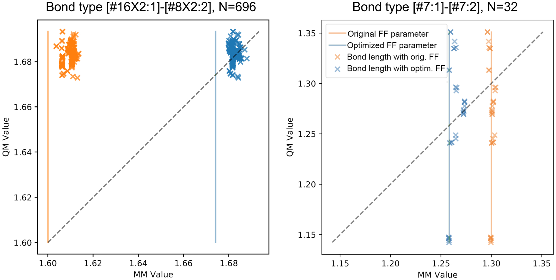
Left: divalent sulfur single-bonded to a divalent oxygen. Right: divalent bond between nitrogens. Vertical line indicates the value of the force field’s equilibrium bond length. Orange and blue indicate results for initial and optimized force field. Dashed: Line of identity.
Relationships among force field equilibrium bond lengths, chemical environment, and strain, may be further explored by examining the lengths of a given bond type across the geometrically optimized conformers of various compounds. Figure 10 illustrates this concept for a generic C-N single bond. The curves in the left panel show the energy-minimized central bond lengths in QM torsion profiles taken from the Roche dataset, including all cases where the central bond is matched by the SMIRKS pattern indicated. The rise and fall of an individual curve indicates a dependence of the central bond length on the torsion angle, and the vertical displacements of the various curves relative to each other indicate the torsion angle-independent differences of central bond lengths between different molecules, or different central bonds in the same molecule. When integrated over all torsion angles, the bond lengths across all instances of the central bond matched by this SMIRKS pattern has a bi- or tri-modal distribution (Figure 10 right panel). This result suggests that this generic bond type ought to be split into at least two or perhaps three more specific types determined by SMIRKS patterns matching more specific chemical environments.
Figure 10. Dependence of bond lengths of a given force field type upon the chemical and conformational environment.

Left: Length of the central bond as a function of the torsion angle in the Roche dataset for central bonds matching the C-N bond type indicated. Each line corresponds to the length of the C-N bond matching the b7 parameter for constrained energy-minimized conformers over a range of torsion angles. Right: Histogram of the observed bond lengths after summing over the torsion angles. Solid line in both panels indicates the force field’s equilibrium bond length for type b7, and dashed lines indicate the lengths for which the bond energy equals 1.2 kcal/mol. The lines labeled in red are b7 in the initial force field, and lines labeled in green are b7 after force field optimization. Example molecules and their given b7 bond(s) are highlighted on the far right, which correspond to typical environments where the bond length is 1.44 Å (orange), 1.46 Å (green), or 1.52 Å (violet).
3.1.3. Vibrational frequencies
Fitting against the training set led to substantial improvements in the accuracy of the vibrational frequencies in the training data, relative to the reference QM results, as evident from a dramatic fall in the vibrational components of the objective function. This is evident in Figure 8b, which shows decreases in error for the sum of squared vibrational frequency differences for individual molecules. Indeed, the improvement from initial results (red) to fitted results (green) appears even more marked than that of optimized geometries (Figure 8a). The distribution of improvements for individual conformations (blue) also shows strong improvement, with only a tiny minority of cases becoming less accurate with fitting. These results correspond to a 67% drop in the RMSE of individual MM vs QM frequencies; i.e., from 119 to 40 cm−1 (Table 3). When the MM vibrational frequencies are permuted to maximize overlap between MM and QM normal modes, the RMSE in the vibrational frequencies is found to decrease by 42% (156 to 90 cm−1) with optimization.
3.1.4. Torsional energy profiles
Fitting also led to improvements in the accuracy of the torsional energy profiles in the training set (Figure 8c), although the improvements (red to green) appear less dramatic than for the geometric and vibrational components discussed above. As for the other objective function components, the improvements observed for many torsions come at the expense of decreased accuracy for some others (blue). The RMSE of the MM torsional energy profiles relative to the QM ones in the training set fell from 2.96 to 1.89 kcal/mol, a 36% drop (Table 3).
It is also of interest to compare the MM and QM potential energy profiles for individual torsion angles across the full training training set, and a full set of comparisons is available in the Supporting Information. Sample plots for a torsional profile that improves with fitting and another that gets worse are provided in Figure 11, left and right panels respectively. Interestingly, the parameter in the second plot occurs 231 times in the training set, so degraded performance is likely not due to lack of sufficient data, but instead to either changes in other portions of the force field, or improved performance on other molecules utilizing this same parameter at the expense of degraded performance for this particular target. Note that most torsional parameters appear in many molecules in the training set, so fitting can improve accuracy for most occurrences while degrading it for others.
Figure 11. Examples of torsional profiles that were improved (left) or degraded (right) by fitting.

Data are for a specific torsion angle in a specific molecule, as detailed below the plot. Blue: QM energy. Orange: force field energy before training. Green: force field energy after training (Parsley). The metadata at the bottom explains which dataset this data is drawn from, and which specific molecule this torsion occurs in, as well as the SMIRKS pattern for the particular torsion being fitted here. The total count of this SMIRKS pattern across the dataset (5) is also shown at the bottom, as well as the parameter ID and the atom indices in the molecule. The full set of plots are available in the release package.93
The greater difficulty of fitting torsional profiles may result from the fact that these are particularly sensitive to nonlocal interactions within the molecules, such as longer-range sterics and electrostatics. Also, defining force field types for torsional terms is more complex than for most other terms in the force field, as multiple torsional terms contribute to the profile around a given bond, and torsional terms include step changes in periodicity. Note, too, that the present fitting process adjusted only amplitudes, and left periodicities and phases unchanged. Adjustment of these additional parameters will clearly be of interest in future rounds of force field development.
3.2. Test Set Results
Results for data outside the training set provide an indication of the transferability of the new parameters and hence of the accuracy that may be expected in actual use. Here, we examine the ability of the new parameters to replicate QM-optimized gas-phase geometries for molecules outside training set, energy differences between gas-phase conformers, physical properties of liquids, and relative protein-ligand binding free energies.
3.2.1. Quantum chemical data
The overall objective function for the test set is lower for Parsley (20,672) than for the initial force field (29,469). The distribution of improvements over the test-set compounds (Figure 8d) shows that the objective function improves for almost all compounds, given that the blue histogram of differences has few positive values. Accordingly, improvements of 6–35% are observed in the terms that contribute to the objective function (Table 3. It is worth noting that the test set exercises 415 out of the 500 parameters. We also grouped the bond lengths, bond angles, and improper dihedrals across test set compound according to their FF types and examined the improvement in accuracy by type, as illustrated for the bond-lengths in Figure 12. The complete figures for bond lengths, bond angles and improper torsion angles can be found in Supporting Information Figures 1–3. Clearly, optimization over the training set led to improved test-improvement for most parameters. Comparable plots for angles and torsions are available in the release package for this force field.94
Figure 12. Bond length RMSE comparison for initial and optimized force fields for the Full Set.

For each bond type (b1, b2…), a gray circle indicates the RMSE of bonds of this type for the initial force field and arrows show the drops (green) or increases (red) in error on going to the new force field. (SMIRKS patterns for these parameter IDs can be retrieved from the force field XML file, openff-1.0.0.offxml.44
We also tested the ability of the Parsley force field to replicate differences among conformations of gas-phase molecules in the test set. Note that this type of data is entirely absent from the training data. Nonetheless, the RMSE for these quantities fell by 12% on going from the initial force field to the new Parsley force field (Table 3). The improvements accuracy are distributed across many compounds, rather than being dominated by improvements for a few, as evident from the histograms in Figure 8e.
3.2.2. Physical properties of organic liquids
We tested Parsley’s ability to model condensed phase properties by using it to compute densities, enthalpies of vaporization, static dielectric constants, enthalpies of mixing, and excess molar volumes, of organic liquids and mixtures, and comparing with experimental data from NIST’s ThermoML. Note that no condensed phase data were used in the fitting process. As shown in Figures 13 and 14, the new Parsley force field offers competitive performance for these data, with marginal, though not statistically significant (by comparison of the root-mean-square errors and their 95% confidence intervals), improvement over the previous SMIRNOFF99frosst 1.1.0 release (Table 4). The overall accuracy also is similar to that of the established GAFF family of force fields. This pattern presumably reflects the fact that these physical properties are not sensitive to the valence parameters optimized here, and that condensed phase data were not used to guide the optimization.
Figure 13. Results of pure property benchmarks.

Liquid properties computed with various force fields, as labeled, are compared with experiment. Density: ρ; dielectric constant: ϵ; heat of vaporization: Hvap;
Figure 14. Results of binary mixture property benchmarks.

Liquid properties computed with various force fields, as labeled, are compared with experiment. Enthalpy of mixing: Hmix; excess molar volume of mixing: Vexcess.
Table 4.
Measures of accuracy of force fields for the physical property benchmarks. RMSE: root-mean-square error; R2: coefficient of determination; τ: Kendall’s tau ranking accuracy metric. Subscripts and superscripts indicate 95% confidence intervals on these statistics.
| Property | Force Field | RMSE | R 2 | τ |
|---|---|---|---|---|
| Vexcess (x) (cm3/mol) | smirnoff99frosst 1.1.0 | |||
| parsley 1.0.0 | ||||
| gaff 1.81 | ||||
| gaff 2.11 | ||||
| Hmix (x) (kJ/mol) | smirnoff99frosst 1.1.0 | |||
| parsley 1.0.0 | ||||
| gaff 1.81 | ||||
| gaff 2.11 | ||||
| Hvap(kJ/mol) | smimoff99frosst 1.1.0 | |||
| parsley 1.0.0 | ||||
| gaff 1.81 | ||||
| gaff 2.11 | ||||
| ρ (g/ml) | smirnoff99frosst 1.1.0 | |||
| parsley 1.0.0 | ||||
| gaff 1.81 | ||||
| gaff 2.11 | ||||
| ϵ | smirnoff99frosst 1.1.0 | |||
| parsley 1.0.0 | ||||
| gaff 1.81 | ||||
| gaff 2.11 |
3.2.3. Protein-ligand binding free energies
The Parsley force field provides competitive accuracy in relative binding free energy calculations for 199 ligands across eight different protein targets, as shown in Figure 15. Indeed, the differences in accuracy across the four force fields examined here are within 95% confidence intervals. It is also important to note that the accuracy of these calculations is strong affected by additional factors, including input structure preparation and sampling time. That said, in terms of mean unsigned error (MUE) of all relative free energy differences ΔΔG, Parsley (MUE = 1.02 kcal mol−1) ranks third, after GAFFv2.1 (MUE = 0.92 kcal mol−1) and OPLS3e (MUE = 0.93 kcal mol−1), and before CGenFF (MUE = 1.09 kcal mol−1). These results indicate that Parsley is a reasonable choice of force field for binding free energy calculations in drug discovery projects.
Figure 15. Results of protein-ligand binding free energy benchmarks.

The predicted relative binding free energies ΔΔG versus the experimental results for 330 alchemical perturbation calculations with four forcefields: Parsley-1.0.0, GAFFv2.1, CGenFFv3.0.1 and OPLS3e. The graphs for the latter three force fields use data reported in Ref. 83. The different colors denote the eight different protein targets.
4. Using and Citing Parsley
The present Parsley force field, formally named openff-1.0.0, can be accessed from Python by installing the Open Force Field Toolkit with the command conda install -c omnia openforcefield openforcefields and then loading the force field as follows:
from openforcefield.typing.engines.smirnoff import ForceField
ff = ForceField (‘openff-1.0.0.offxml’)
The default version of Parsley includes hydrogen bond length constraints, which allow use of the typical 2–4 fs timestep in molecular dynamics simulations. A second version without these constraints, which is suitable for geometry optimizations and single-point energy calculations, may be accessed as follows:
ff = ForceField (‘openff_unconstrained-1.0.0.offxml’
)
An example of the use of Parsley to run a molecular dynamics simulation can be found in Supporting Information section 3. Alternatively, the force field files themselves can be found under the openforcefields/offxml subdirectory of the openforcefields GitHub repository.95
The present Parsley version may be referred to as “Open Force Field (OpenFF) Parsley Force Field (v1.0.0)” on first reference, and “Parsley” thereafter. Newer Open Force Fields are in development, and updates in the OpenFF 1.x series will also be referred to as Parsley, while new major versions will receive updated codenames. To cite Parsley, please reference the latest version of this article and the DOI of the force field version you use. This information is available in the OpenForceField repository,95 and the present version may be cited as.44
To provide feedback on the performance of the OpenFF force fields, we highly recommend using the issue tracker at http://github.com/openforcefield/openforcefields. For toolkit feedback, use http://github.com/openforcefield/openforcefield. Alternatively, inquiries may be e-mailed to support@openforcefield.org, though responses to e-mails sent to this address may be delayed and GitHub issues receive higher priority. For information on getting started with OpenFF, please see the documentation linked at http://github.com/openforcefield/openforcefield, and note the availability of several introductory examples.
5. Conclusions and Directions
We have described a methodology to derive new simulation force fields and an initial application of this infrastructure to create OpenFF 1.0.0 (codenamed Parsley), a SMIRNOFF force field with bonded terms optimized against a range of gas-phase QM reference data. For both training and test sets, Parsley provides more accurate molecular geometries and conformational energetics, while preserving accuracy for a range of condensed phase properties. Importantly, it also yields highly competitive accuracy in calculations of relative protein-ligand binding free energies. This work lays a foundation for efficient iterative force field improvement, which is already underway in subsequent releases (OpenFF 1.1, 1.2, 1.2.1 and 1.3,37–41 to be described elsewhere). This work could also be naturally extended to automatically derive molecule-specific (i.e. “bespoke”) parameters96 and we are actively developing software tools for this application.
In the near term, we aim to extend the optimization to nonbonded interaction parameters and incorporate expanded training and testing data sets. Later, we plan to address issues related to the definitions of chemical types and elaboration of the functional form, such as by the addition of off-center partial charges and incorporation of an explicit treatment of electronic polarizability. At the same time, we hope that the associated open release of our datasets and infrastructure will enable independent use of these data and tools to advance force field science.
Supplementary Material
Figure 5.

Example torsions selected for 1D torsion scans in the Roche TorsionDrive dataset. H, white; C, gray; N, blue; O, red; S, yellow; F, green (lower middle); Cl, green (lower left).
Table 1.
Summary of quantum chemical calculations used to fit the force field valence parameters in this work. These publicly available datasets are stored on the MolSSI QCArchive Server (MQCAS)
| Roche Set | Coverage Set | ||
|---|---|---|---|
| Compounds | 468 | 80 | |
| Cmpds × Prot. States | 468 | 233 | |
| Opt. Geom. | Geometries | 936 | 831 |
| Dataset Name | OpenFF Optimization Set 1 | SMIRNOFF Coverage Set 1 | |
| Vib. Freq. | Frequency Sets | 660 | 235 |
| Dataset Name | OpenFF Optimization Set 1 | SMIRNOFF Coverage Set 1 | |
| Tors. Scans | Energy Profiles | 669 | 417 |
| Dataset Name | OpenFF Group 1 Torsions | SMIRNOFF Coverage Torsion Set 1 |
6. Acknowledgements
In this work, we stand on the shoulders of giants in the force field development community, and it would be impossible to provide a complete list of all those whose work we have benefitted from. However, we are particularly indebted to the AMBER force field community, from which we derived the initial small molecule force fields which provided the starting point for this work. We thank the Open Force Field Consortium for funding, including our industry partners as listed at the Open Force Field website.97 We gratefully acknowledge Owen Madin and Karmen Condic-Jurkic for helpful discussions, along with all current and former members of the Open Force Field Initiative and the Open Force Field Scientific Advisory Board. We thank Vytautas Gapsys for assistance with the binding free energy calculations and for the insightful discussions. We thank the National Institutes of Health (NIGMS R01GM132386) for funding longer-term aspects of this initiative. MKG acknowledges funding from National Institute of General Medical Sciences (GM061300). LPW and YQ acknowledge support from ACS PRF 58158-DNI6. MRS and JDC acknowledge support from NSF CHE-1738975. DGAS acknowledges funding from the U. S. National Science Foundation (NSF) grant ACI-1547580. These findings are solely of the authors and do not necessarily represent the views of the NIH or NSF.
7. Disclosures
The Chodera laboratory receives or has received funding from multiple sources, including the National Institutes of Health, the National Science Foundation, the Parker Institute for Cancer Immunotherapy, Relay Therapeutics, Entasis Therapeutics, Silicon Therapeutics, EMD Serono (Merck KGaA), AstraZeneca, Vir Biotechnology, XtalPi, Foresite Labs, the Molecular Sciences Software Institute, the Starr Cancer Consortium, the Open Force Field Consortium, Cycle for Survival, a Louis V. Gerstner Young Investigator Award, and the Sloan Kettering Institute. A complete funding history for the Chodera lab can be found at http://choderalab.org/funding.
JDC is a current member of the Scientific Advisory Board of OpenEye Scientific Software and scientific consultant to Foresite Labs.
MRS is an Open Science Fellow for Silicon Therapeutics.
MKG has an equity interest in and is a cofounder and scientific advisor of VeraChem LLC.
DLM is a current member of the Scientific Advisory Board of OpenEye Scientific Software and an Open Science Fellow for Silicon Therapeutics.
Footnotes
Supporting Information Available
The supporting information document contains links to scripts and resources for training, testing, and running simulations using the Parsley force field; simulation procedures for physical properties of organic liquids; and optimized geometry RMSEs for the full test set grouped by parameter type. This information is available free of charge via the Internet at http://pubs.acs.org.
References
- [1].Coleman RG, Carchia M, Sterling T, Irwin JJ, Shoichet BK. Ligand Pose and Orientational Sampling in Molecular Docking. PLOS ONE. 2013. 10; 8(10):1–19. 10.1371/journal.pone.0075992, doi: 10.1371/journal.pone.0075992. [DOI] [PMC free article] [PubMed] [Google Scholar]
- [2].Allen WJ, Balius TE, Mukherjee S, Brozell SR, Moustakas DT, Lang PT, Case DA, Kuntz ID, Rizzo RC. DOCK 6: Impact of new features and current docking performance. Journal of Computational Chemistry. 2015; 36(15):1132–1156. https://onlinelibrary.wiley.com/doi/abs/10.1002/jcc.23905, doi: 10.1002/jcc.23905. [DOI] [PMC free article] [PubMed] [Google Scholar]
- [3].Österberg F, Morris GM, Sanner MF, Olson AJ, Goodsell DS. Automated docking to multiple target structures: Incorporation of protein mobility and structural water heterogeneity in AutoDock. Proteins: Structure, Function, and Bioinformatics. 2002; 46(1):34–40. https://onlinelibrary.wiley.com/doi/abs/10.1002/prot.10028, doi: 10.1002/prot.10028. [DOI] [PubMed] [Google Scholar]
- [4].Friesner RA, Banks JL, Murphy RB, Halgren TA, Klicic JJ, Mainz DT, Repasky MP, Knoll EH, Shelley M, Perry JK, Shaw DE, Francis P, Shenkin PS. Glide: A New Approach for Rapid, Accurate Docking and Scoring. 1. Method and Assessment of Docking Accuracy. Journal of Medicinal Chemistry. 2004; 47(7):1739–1749. 10.1021/jm0306430, doi: 10.1021/jm0306430 [DOI] [PubMed] [Google Scholar]
- [5].Jain AN. Surflex: Fully Automatic Flexible Molecular Docking Using a Molecular Similarity-Based Search Engine. Journal of Medicinal Chemistry. 2003; 46(4):499–511. 10.1021/jm020406h, doi: 10.1021/jm020406h [DOI] [PubMed] [Google Scholar]
- [6].Jones G, Willett P, Glen RC, Leach AR, Taylor R. Development and validation of a genetic algorithm for flexible docking. Journal of Molecular Biology. 1997; 267(3):727 – 748. http://www.sciencedirect.com/science/article/pii/S0022283696908979, doi: 10.1006/jmbi.1996.0897. [DOI] [PubMed] [Google Scholar]
- [7].McGann MR, Almond HR, Nicholls A, Grant JA, Brown FK. Gaussian docking functions. Biopolymers. 2003; 68(1):76–90. https://onlinelibrary.wiley.com/doi/abs/10.1002/bip.10207, doi: 10.1002/bip.10207. [DOI] [PubMed] [Google Scholar]
- [8].Lamb ML, Jorgensen WL. Computational approaches to molecular recognition. Current Opinion in Chemical Biology. 1997; 1(4):449 – 457. http://www.sciencedirect.com/science/article/pii/S1367593197800385, doi: 10.1016/S1367-5931(97)80038-5. [DOI] [PubMed] [Google Scholar]
- [9].Gilson MK, Zhou HX. Calculation of Protein-Ligand Binding Affinities. Annual Review of Biophysics and Biomolecular Structure. 2007; 36(1):21–42. 10.1146/annurev.biophys.36.040306.132550, doi: 10.1146/annurev.biophys.36.040306.132550. [DOI] [PubMed] [Google Scholar]
- [10].Gallicchio E, Levy RM. Recent theoretical and computational advances for modeling protein–ligand binding affinities. In: Christov C, editor. Computational chemistry methods in structural biology, vol. 85 of Advances in Protein Chemistry and Structural Biology Academic Press; 2011.p. 27 – 80. http://www.sciencedirect.com/science/article/pii/B9780123864857000028, doi: 10.1016/B978-0-12-386485-7.00002-8. [DOI] [PMC free article] [PubMed] [Google Scholar]
- [11].Huggins DJ, Biggin PC, Dämgen MA, Essex JW, Harris SA, Henchman RH, Khalid S, Kuzmanic A, Laughton CA, Michel J, Mulholland AJ, Rosta E, Sansom MSP, van der Kamp MW. Biomolecular simulations: From dynamics and mechanisms to computational assays of biological activity. WIREs Computational Molecular Science. 2019; 9(3):e1393. https://onlinelibrary.wiley.com/doi/abs/10.1002/wcms.1393, doi: 10.1002/wcms.1393. [DOI] [Google Scholar]
- [12].Wang L, Wu Y, Deng Y, Kim B, Pierce L, Krilov G, Lupyan D, Robinson S, Dahlgren MK, Greenwood J, Romero DL, Masse C, Knight JL, Steinbrecher T, Beuming T, Damm W, Harder E, Sherman W, Brewer M, Wester R, et al. Accurate and Reliable Prediction of Relative Ligand Binding Potency in Prospective Drug Discovery by Way of a Modern Free-Energy Calculation Protocol and Force Field. Journal of the American Chemical Society. 2015; 137(7):2695–2703. 10.1021/ja512751q, doi: 10.1021/ja512751q. [DOI] [PubMed] [Google Scholar]
- [13].Cournia Z, Allen B, Sherman W. Relative Binding Free Energy Calculations in Drug Discovery: Recent Advances and Practical Considerations. Journal of Chemical Information and Modeling. 2017; 57(12):2911–2937. 10.1021/acs.jcim.7b00564, doi: 10.1021/acs.jcim.7b00564 [DOI] [PubMed] [Google Scholar]
- [14].Schindler C, Baumann H, Blum A, Böse D, Buchstaller HP, Burgdorf L, Cappel D, Chekler E, Czodrowski P, Dorsch D, Eguida M, Follows B, Fuchß T, Grädler U, Gunera J, Johnson T, Lebrun CJ, Karra S, Klein M, Kötzner L, et al. , Large-Scale Assessment of Binding Free Energy Calculations in Active Drug Discovery Projects; 2020. https://chemrxiv.org/articles/preprint/Large-Scale_Assessment_of_Binding_Free_Energy_Calculations_in_Active_Drug_Discovery_Projects/11364884, doi: 10.26434/chemrxiv.11364884.v2. [DOI] [PubMed] [Google Scholar]
- [15].Cournia Z, Allen BK, Beuming T, Pearlman DA, Radak BK, Sherman W. Rigorous Free Energy Simulations in Virtual Screening. Journal of Chemical Information and Modeling. 2020; 60(9):4153–4169. 10.1021/acs.jcim.0c00116, doi: 10.1021/acs.jcim.0c00116 [DOI] [PubMed] [Google Scholar]
- [16].Cornell WD, Cieplak P, Bayly CI, Gould IR, Merz KM, Ferguson DM, Spellmeyer DC, Fox T, Caldwell JW, Kollman PA. A Second Generation Force Field for the Simulation of Proteins, Nucleic Acids, and Organic Molecules. Journal of the American Chemical Society. 1995; 117(19):5179–5197. 10.1021/ja00124a002, doi: 10.1021/ja00124a002. [DOI] [Google Scholar]
- [17].MacKerell AD, Bashford D, Bellott M, Dunbrack RL, Evanseck JD, Field MJ, Fischer S, Gao J, Guo H, Ha S, Joseph-McCarthy D, Kuchnir L, Kuczera K, Lau FTK, Mattos C, Michnick S, Ngo T, Nguyen DT, Prodhom B, Reiher WE, et al. All-Atom Empirical Potential for Molecular Modeling and Dynamics Studies of Proteins. The Journal of Physical Chemistry B. 1998; 102(18):3586–3616. 10.1021/jp973084f, doi: 10.1021/jp973084f [DOI] [PubMed] [Google Scholar]
- [18].Foloppe N, MacKerell AD Jr. All-atom empirical force field for nucleic acids: I. Parameter optimization based on small molecule and condensed phase macromolecular target data. Journal of Computational Chemistry. 2000; 21(2):86–104. doi: . [DOI] [Google Scholar]
- [19].MacKerell AD Jr, Banavali NK. All-atom empirical force field for nucleic acids: II. Application to molecular dynamics simulations of DNA and RNA in solution. Journal of Computational Chemistry. 2000; 21(2):105–120. doi: . [DOI] [Google Scholar]
- [20].Hornak V, Abel R, Okur A, Strockbine B, Roitberg A, Simmerling C. Comparison of multiple Amber force fields and development of improved protein backbone parameters. Proteins: Structure, Function, and Bioinformatics. 2006; 65(3):712–725. https://onlinelibrary.wiley.com/doi/abs/10.1002/prot.21123, doi: 10.1002/prot.21123. [DOI] [PMC free article] [PubMed] [Google Scholar]
- [21].Lindorff-Larsen K, Piana S, Palmo K, Maragakis P, Klepeis JL, Dror RO, Shaw DE. Improved side-chain torsion potentials for the Amber ff99SB protein force field. Proteins: Structure, Function, and Bioinformatics. 2010; 78(8):1950–1958. https://onlinelibrary.wiley.com/doi/abs/10.1002/prot.22711, doi: 10.1002/prot.22711. [DOI] [PMC free article] [PubMed] [Google Scholar]
- [22].Wang LP, McKiernan KA, Gomes J, Beauchamp KA, Head-Gordon T, Rice JE, Swope WC, Martínez TJ, Pande VS. Building a More Predictive Protein Force Field: A Systematic and Reproducible Route to AMBER-FB15. The Journal of Physical Chemistry B. 2017; 121(16):4023–4039. 10.1021/acs.jpcb.7b02320, doi: 10.1021/acs.jpcb.7b02320 [DOI] [PMC free article] [PubMed] [Google Scholar]
- [23].Oostenbrink C, Villa A, Mark AE, Van Gunsteren WF. A biomolecular force field based on the free enthalpy of hydration and solvation: The GROMOS force-field parameter sets 53A5 and 53A6. Journal of Computational Chemistry. 2004; 25(13):1656–1676. https://onlinelibrary.wiley.com/doi/abs/10.1002/jcc.20090, doi: 10.1002/jcc.20090. [DOI] [PubMed] [Google Scholar]
- [24].Shi Y, Xia Z, Zhang J, Best R, Wu C, Ponder JW, Ren P. Polarizable Atomic Multipole-Based AMOEBA Force Field for Proteins. Journal of Chemical Theory and Computation. 2013; 9(9):4046–4063. 10.1021/ct4003702, doi: 10.1021/ct4003702 [DOI] [PMC free article] [PubMed] [Google Scholar]
- [25].Kim S, Thiessen PA, Bolton EE, Chen J, Fu G, Gindulyte A, Han L, He J, He S, Shoemaker BA, Wang J, Yu B, Zhang J, Bryant SH. PubChem Substance and Compound databases. Nucleic Acids Research. 2016. January; 44(D1):D1202–D1213. https://academic.oup.com/nar/article/44/D1/D1202/2503131, doi: 10.1093/nar/gkv951, publisher: Oxford Academic. [DOI] [PMC free article] [PubMed] [Google Scholar]
- [26].Wang J, Wolf RM, Caldwell JW, Kollman PA, Case DA. Development and testing of a general amber force field. Journal of Computational Chemistry. 2004. July; 25(9):1157–1174. doi: 10.1002/jcc.20035. [DOI] [PubMed] [Google Scholar]
- [27].Vanommeslaeghe K, Hatcher E, Acharya C, Kundu S, Zhong S, Shim J, Darian E, Guvench O, Lopes P, Vorobyov I, Mackerell AD. CHARMM general force field: A force field for drug-like molecules compatible with the CHARMM all-atom additive biological force fields. Journal of Computational Chemistry. 2010; 31(4). doi: 10.1002/jcc.21367. [DOI] [PMC free article] [PubMed] [Google Scholar]
- [28].Jorgensen WL, Maxwell DS, Tirado-Rives J. Development and Testing of the OPLS All-Atom Force Field on Conformational Energetics and Properties of Organic Liquids. Journal of the American Chemical Society. 1996; 118(45):11225–11236. doi: 10.1021/ja9621760. [DOI] [Google Scholar]
- [29].Fennell CJ, Wymer KL, Mobley DL. A Fixed-Charge Model for Alcohol Polarization in the Condensed Phase, and Its Role in Small Molecule Hydration. The Journal of Physical Chemistry B. 2014; 118(24):6438–6446. 10.1021/jp411529h, doi: 10.1021/jp411529h [DOI] [PMC free article] [PubMed] [Google Scholar]
- [30].Henriksen NM, Fenley AT, Gilson MK. Computational Calorimetry: High-Precision Calculation of Host–Guest Binding Thermodynamics. Journal of Chemical Theory and Computation. 2015; 11(9):4377–4394. 10.1021/acs.jctc.5b00405, doi: 10.1021/acs.jctc.5b00405 [DOI] [PMC free article] [PubMed] [Google Scholar]
- [31].Yin J, Henriksen NM, Muddana HS, Gilson MK. Bind3P: Optimization of a Water Model Based on Host–Guest Binding Data. Journal of Chemical Theory and Computation. 2018; 14(7):3621–3632. 10.1021/acs.jctc.8b00318, doi: 10.1021/acs.jctc.8b00318 [DOI] [PMC free article] [PubMed] [Google Scholar]
- [32].Kenney IM, Beckstein O, Iorga BI. Prediction of cyclohexane-water distribution coefficients for the SAMPL5 data set using molecular dynamics simulations with the OPLS-AA force field. Journal of computer-aided molecular design. 2016. November; 30(11):1045—1058. 10.1007/s10822-016-9949-5, doi: 10.1007/s10822-016-9949-5. [DOI] [PubMed] [Google Scholar]
- [33].Rizzi A, Murkli S, McNeill JN, Yao W, Sullivan M, Gilson MK, Chiu MW, Isaacs L, Gibb BC, Mobley DL, Chodera JD. Overview of the SAMPL6 host–guest binding affinity prediction challenge. Journal of Computer-Aided Molecular Design. ; 32(10):937–963. 10.1007/s10822-018-0170-6, doi: 10.1007/s10822-018-0170-6. [DOI] [PMC free article] [PubMed] [Google Scholar]
- [34].Roos K, Wu C, Damm W, Reboul M, Stevenson JM, Lu C, Dahlgren MK, Mondal S, Chen W, Wang L, Abel R, Friesner RA, Harder ED. OPLS3e: Extending Force Field Coverage for Drug-Like Small Molecules. Journal of Chemical Theory and Computation. 2019. March; 15(3):1863–1874. 10.1021/acs.jctc.8b01026, doi: 10.1021/acs.jctc.8b01026. [DOI] [PubMed] [Google Scholar]
- [35].Mobley DL, Bannan CC, Rizzi A, Bayly CI, Chodera JD, Lim VT, Lim NM, Beauchamp KA, Slochower DR, Shirts MR, Gilson MK, Eastman PK. Escaping Atom Types in Force Fields Using Direct Chemical Perception. Journal of Chemical Theory and Computation. 2018; 14(11):6076–6092. 10.1021/acs.jctc.8b00640, doi: 10.1021/acs.jctc.8b00640 [DOI] [PMC free article] [PubMed] [Google Scholar]
- [36].Bayly C, McKay D, Truchon J, An Informal AMBER Small Molecule Force Field: Parm@ Frosst; 2010. http://www.ccl.net/cca/data/parm_at_Frosst/.
- [37].Jang H, Update on Parsley Minor Releases (Openff-1.1.0, 1.2.0); 2020. doi: 10.5281/zenodo.3781313. [DOI] [Google Scholar]
- [38].Jang H, Maat J, Qiu Y, Smith DGA, Boothroyd S, Wagner J, Bannan CC, Gokey T, Lim VT, Lucas X, Tjanaka B, Shirts MR, Gilson MK, Chodera JD, Bayly CI, Mobley DL, Wang LP, Openforcefield/Openforcefields: Version 1.2.0 “Parsley” Update; 2020. doi: 10.5281/zenodo.3872244. Zenodo. [DOI] [Google Scholar]
- [39].Jang H, Maat J, Qiu Y, Smith DGA, Boothroyd S, Wagner J, Bannan CC, Gokey T, Lim VT, Lucas X, Tjanaka B, Shirts MR, Gilson MK, Chodera JD, Bayly CI, Mobley DL, Wang LP, Openforcefield/Openforcefields: Version 1.1.0 “Parsley” Update; 2020. doi: 10.5281/zenodo.3695094. Zenodo. [DOI] [Google Scholar]
- [40].Wagner J, Thompson M, Dotson D, hyejang, Rodríguez-Guerra J, Openforcefield/Openforcefields: Version 1.2.1 “Parsley” Update; 2020. doi: 10.5281/zenodo.4021623. Zenodo. [DOI] [Google Scholar]
- [41].Wagner J, Thompson M, Dotson D, hyejang, Rodríguez-Guerra J, Openforcefield/Openforcefields: Version 1.3.0 “Parsley” Update; 2020. doi: 10.5281/zenodo.4118484. Zenodo. [DOI] [Google Scholar]
- [42].Wang J, Cieplak P, Kollman PA. How well does a restrained electrostatic potential (RESP) model perform in calculating conformational energies of organic and biological molecules? Journal of Computational Chemistry. 2000; 21(12):1049–1074. doi: . [DOI] [Google Scholar]
- [43].Wang LP, Martinez TJ, Pande VS. Building Force Fields: An Automatic, Systematic, and Reproducible Approach. The Journal of Physical Chemistry Letters. 2014; 5(11):1885–1891. 10.1021/jz500737m, doi: 10.1021/jz500737m. [DOI] [PMC free article] [PubMed] [Google Scholar]
- [44].Wagner J, openforcefield/openforcefields: Version 1.0.0 “Parsley”. Zenodo; 2019. 10.5281/zenodo.3483227, doi: 10.5281/zenodo.3483227. [DOI] [Google Scholar]
- [45].Vilar S, Cozza G, Moro S. Medicinal Chemistry and the Molecular Operating Environment (MOE): Application of QSAR and Molecular Docking to Drug Discovery. Current topics in medicinal chemistry. 2008. December; 8(18):1555–1572. doi: { 10.2174/156802608786786624}. [DOI] [PubMed] [Google Scholar]
- [46].eMolecules Plus Database Download; 2013. https://www.emolecules.com/info/plus/download-database.
- [47].MolSSI QCFractal Documentation; 2019. https://qcfractal.readthedocs.io.
- [48].MolSSI QCArchive web page; 2020. https://qcarchive.molssi.org/.
- [49].Smith DGA, Altarawy D, Burns LA, Welborn M, Naden LN, Ward L, Ellis S, Pritchard BP, Crawford TD. The MolSSI QCArchive project: An open-source platform to compute, organize, and share quantum chemistry data. WIREs Computational Molecular Science. ; n/a(n/a):e1491. https://onlinelibrary.wiley.com/doi/abs/10.1002/wcms.1491, doi: 10.1002/wcms.1491. [DOI] [Google Scholar]
- [50].Godbout N, Salahub DR, Andzelm J, Wimmer E. Optimization of Gaussian-type basis sets for local spin density functional calculations. Part I. Boron through neon, optimization technique and validation. Canadian Journal of Chemistry. 1992; 70(2):560–571. 10.1139/v92-079, doi: 10.1139/v92-079. [DOI] [Google Scholar]
- [51].Becke AD. Density-functional thermochemistry. III. The role of exact exchange. The Journal of Chemical Physics. 1993; 98(7):5648–5652. 10.1063/1.464913, doi: 10.1063/1.464913. [DOI] [Google Scholar]
- [52].Grimme S, Antony J, Ehrlich S, Krieg H. A consistent and accurate ab initio parametrization of density functional dispersion correction (DFT-D) for the 94 elements H-Pu. The Journal of Chemical Physics. 2010; 132(15):154104. 10.1063/1.3382344, doi: 10.1063/1.3382344. [DOI] [PubMed] [Google Scholar]
- [53].Grimme S, Ehrlich S, Goerigk L. Effect of the damping function in dispersion corrected density functional theory. Journal of Computational Chemistry. 2011; 32(7):1456–1465. https://onlinelibrary.wiley.com/doi/abs/10.1002/jcc.21759, doi: 10.1002/jcc.21759. [DOI] [PubMed] [Google Scholar]
- [54].Řezáč J, Bím D, Gutten O, Rulíšek L. Toward Accurate Conformational Energies of Smaller Peptides and Medium-Sized Macrocycles: MPCONF196 Benchmark Energy Data Set. Journal of Chemical Theory and Computation. 2018; 14(3):1254–1266. 10.1021/acs.jctc.7b01074, doi: 10.1021/acs.jctc.7b01074 [DOI] [PubMed] [Google Scholar]
- [55].Kesharwani MK, Karton A, Martin JML. Benchmark ab Initio Conformational Energies for the Proteinogenic Amino Acids through Explicitly Correlated Methods. Assessment of Density Functional Methods. Journal of Chemical Theory and Computation. 2016; 12(1):444–454. 10.1021/acs.jctc.5b01066, doi: 10.1021/acs.jctc.5b01066 [DOI] [PubMed] [Google Scholar]
- [56].Weigend F, Ahlrichs R. Balanced basis sets of split valence, triple zeta valence and quadruple zeta valence quality for H to Rn: Design and assessment of accuracy. Phys Chem Chem Phys. 2005; 7:3297–3305. 10.1039/B508541A, doi: 10.1039/B508541A. [DOI] [PubMed] [Google Scholar]
- [57].Tian C, Kasavajhala K, Belfon KAA, Raguette L, Huang H, Migues AN, Bickel J, Wang Y, Pincay J, Wu Q, Simmerling C. ff19SB: Amino-Acid-Specific Protein Backbone Parameters Trained against Quantum Mechanics Energy Surfaces in Solution. Journal of Chemical Theory and Computation. 2020; 16(1):528–552. doi: 10.1021/acs.jctc.9b00591. [DOI] [PubMed] [Google Scholar]
- [58].Stern CD, Bayly CI, Smith DGA, Fass J, Wang LP, Mobley DL, Chodera JD. Capturing non-local through-bond effects when fragmenting molecules for quantum chemical torsion scans. bioRxiv. 2020; https://www.biorxiv.org/content/early/2020/08/28/2020.08.27.270934, doi: 10.1101/2020.08.27.270934. [DOI] [Google Scholar]
- [59].Wang LP, Song C. Geometry optimization made simple with translation and rotation coordinates. J Chem Phys. 2016. June; 144(21):214108. https://aip.scitation.org/doi/abs/10.1063/1.4952956, doi: 10.1063/1.4952956. [DOI] [PubMed] [Google Scholar]
- [60].Parrish RM, Burns LA, Smith DGA, Simmonett AC, DePrince AE, Hohenstein EG, Bozkaya U, Sokolov AY, Di Remigio R, Richard RM, Gonthier JF, James AM, McAlexander HR, Kumar A, Saitow M, Wang X, Pritchard BP, Verma P, Schaefer HF, Patkowski K, et al. Psi4 1.1: An Open-Source Electronic Structure Program Emphasizing Automation, Advanced Libraries, and Interoperability. Journal of Chemical Theory and Computation. 2017; 13(7):3185–3197. 10.1021/acs.jctc.7b00174, doi: 10.1021/acs.jctc.7b00174 [DOI] [PMC free article] [PubMed] [Google Scholar]
- [61].Smith DGA, Burns LA, Simmonett AC, Parrish RM, Schieber MC, Galvelis R, Kraus P, Kruse H, Di Remigio R, Alenaizan A, James AM, Lehtola S, Misiewicz JP, Scheurer M, Shaw RA, Schriber JB, Xie Y, Glick ZL, Sirianni DA, O’Brien JS, et al. PSI4 1.4: Open-source software for high-throughput quantum chemistry. The Journal of Chemical Physics. 2020; 152(18):184108. 10.1063/5.0006002, doi: 10.1063/5.0006002. [DOI] [PMC free article] [PubMed] [Google Scholar]
- [62].Mobley DL, Wagner J, Chodera J, Bannan C, Rizzi A, Camila, Bayly C, SimonBoothroyd, Lim NM, Lim V, Zhao Y, Lee-Ping, openforcefield/openforcefield: 0.4.1 Bugfix Release. Zenodo; 2019. 10.5281/zenodo.3266364, doi: 10.5281/zenodo.3266364. [DOI] [Google Scholar]
- [63].Qiu Y, Smith DGA, Stern CD, Feng M, Jang H, Wang LP. Driving torsion scans with wavefront propagation. The Journal of Chemical Physics. 2020; 152(24):244116. doi: 10.1063/5.0009232. [DOI] [PMC free article] [PubMed] [Google Scholar]
- [64].Paton RS, Goodman JM. Hydrogen Bonding and Pi-Stacking: How Reliable are Force Fields? A Critical Evaluation of Force Field Descriptions of Nonbonded Interactions. Journal of Chemical Information and Modeling. 2009; 49(4):944–955. doi: 10.1021/ci900009f. [DOI] [PubMed] [Google Scholar]
- [65].McGibbon RT, Beauchamp KA, Harrigan MP, Klein C, Swails JM, Hernández CX, Schwantes CR, Wang LP, Lane TJ, Pande VS. MDTraj: A Modern Open Library for the Analysis of Molecular Dynamics Trajectories. Biophysical Journal. 2015; 109(8):1528 – 1532. doi: 10.1016/j.bpj.2015.08.015. [DOI] [PMC free article] [PubMed] [Google Scholar]
- [66].Harder E, Damm W, Maple J, Wu C, Reboul M, Xiang JY, Wang L, Lupyan D, Dahlgren MK, Knight JL, et al. OPLS3: a force field providing broad coverage of drug-like small molecules and proteins. Journal of chemical theory and computation. 2016; 12(1):281–296. [DOI] [PubMed] [Google Scholar]
- [67].Cerutti DS, Swope WC, Rice JE, Case DA. ff14ipq: A self-consistent force field for condensed-phase simulations of proteins. Journal of chemical theory and computation. 2014; 10(10):4515–4534. [DOI] [PMC free article] [PubMed] [Google Scholar]
- [68].Zgarbova M, Otyepka M, Sponer J, Mladek A, Banas P, Cheatham III TE, Jurecka P. Refinement of the Cornell et al. nucleic acids force field based on reference quantum chemical calculations of glycosidic torsion profiles. Journal of chemical theory and computation. 2011; 7(9):2886–2902. [DOI] [PMC free article] [PubMed] [Google Scholar]
- [69].Robertson MJ, Tirado-Rives J, Jorgensen WL. Improved Peptide and Protein Torsional Energetics with the OPLS-AA Force Field. Journal of Chemical Theory and Computation. 2015; 11(7):3499–3509. doi: 10.1021/acs.jctc.5b00356. [DOI] [PMC free article] [PubMed] [Google Scholar]
- [70].Wang LP, McKiernan KA, Gomes J, Beauchamp KA, Head-Gordon T, Rice JE, Swope WC, Martínez TJ, Pande VS. Building a More Predictive Protein Force Field: A Systematic and Reproducible Route to AMBER-FB15. J Phys Chem B. 2017. April; 121(16):4023–4039. 10.1021/acs.jpcb.7b02320, doi: 10.1021/acs.jpcb.7b02320. [DOI] [PMC free article] [PubMed] [Google Scholar]
- [71].Development version of ForceBalance based on v1.6.0 used for 1.0.0 valence parameter fitting; 2019. https://github.com/leeping/forcebalance/tree/5b3a65d1baefe17625c9b05c0db5d27458c5344a. [Google Scholar]
- [72].Lim VT, Hahn DF, Tresadern G, Bayly CI, Mobley D, Benchmark Assessment of Molecular Geometries and Energies from Small Molecule Force Fields. ChemRxiv; 2020. doi: 10.26434/chemrxiv.12551867.v2. [DOI] [PMC free article] [PubMed] [Google Scholar]
- [73].Ehrman JN, Bannan CC, Lim VT, Thi N, Kyu DY, Mobley DL, Improving Force Fields by Identifying and Characterizing Small Molecules with Parameter Inconsistencies. Zenodo; 2019. 10.5281/zenodo.3385278, doi: 10.5281/zenodo.3385278. [DOI] [PMC free article] [PubMed] [Google Scholar]
- [74].Ehrman JN, Lim VT, Bannan CC, Thi N, Kyu DY, Mobley DL. Improving Small Molecule Force Fields by Identifying and Characterizing Small Molecules with Inconsistent Parameters. J Comput Aided Mol Des. 2021. March; 35(3):271–284. doi: 10.1007/s10822-020-00367-1. [DOI] [PMC free article] [PubMed] [Google Scholar]
- [75].Sure R, Grimme S. Corrected small basis set Hartree-Fock method for large systems. Journal of Computational Chemistry. 2013; 34(19):1672–1685. https://onlinelibrary.wiley.com/doi/abs/10.1002/jcc.23317, doi: 10.1002/jcc.23317. [DOI] [PubMed] [Google Scholar]
- [76].Sresht V, Rai B, PfizerRD torsional-strain, Calculation of Torsional Strain Energy; 2019. https://github.com/PfizerRD/torsional-strain. [Google Scholar]
- [77].Sterling T, Irwin JJ. ZINC 15 – Ligand Discovery for Everyone. Journal of Chemical Information and Modeling. 2015; 55(11):2324–2337. 10.1021/acs.jcim.5b00559, doi: 10.1021/acs.jcim.5b00559 [DOI] [PMC free article] [PubMed] [Google Scholar]
- [78].QCArchive Basic Examples, Optimization Datasets;. https://qcarchivetutorials.readthedocs.io/en/latest/basic_examples/optimization_datasets.html/.
- [79].Frenkel M, Chiroco RD, Diky V, Dong Q, Marsh KN, Dymond JH, Wakeham WA, Stein SE, Königsberger E, Goodwin AH. XML-based IUPAC standard for experimental, predicted, and critically evaluated thermodynamic property data storage and capture (ThermoML) (IUPAC Recommendations 2006). Pure and Applied Chemistry,. 2006; 78(3):541–612. 10.1351/pac200678030541, doi: 10.1351/pac200678030541. [DOI] [Google Scholar]
- [80].Jorgensen WL, Chandrasekhar J, Madura JD, Impey RW, Klein ML. Comparison of simple potential functions for simulating liquid water. The Journal of Chemical Physics. 1983; 79(2):926–935. 10.1063/1.445869, doi: 10.1063/1.445869. [DOI] [Google Scholar]
- [81].Beauchamp KA, Behr JM, Rustenburg AS, Bayly CI, Kroenlein K, Chodera JD. Toward Automated Benchmarking of Atomistic Force Fields: Neat Liquid Densities and Static Dielectric Constants from the ThermoML Data Archive. The Journal of Physical Chemistry B. 2015; 119(40):12912–12920. doi: 10.1021/acs.jpcb.5b06703. [DOI] [PMC free article] [PubMed] [Google Scholar]
- [82].Hahn DF, Bayly CI, Macdonald HEB, Chodera JD, Mey ASJS, Mobley DL, Benito LP, Schindler CEM, Tresadern G, Warren GL. Best practices for constructing, preparing, and evaluating protein-ligand binding affinity benchmarks. arXiv:210506222 [physics, q-bio]. 2021. May; http://arxiv.org/abs/2105.06222, arXiv: 2105.06222. [DOI] [PMC free article] [PubMed] [Google Scholar]
- [83].Gapsys V, Pérez-Benito L, Aldeghi M, Seeliger D, van Vlijmen H, Tresadern G, de Groot BL. Large scale relative protein ligand binding affinities using non-equilibrium alchemy. Chemical Science. 2020; 11(4):1140–1152. http://xlink.rsc.org/?DOI=C9SC03754C, doi: 10.1039/C9SC03754C, tex.ids: gapsys_large_2020a, gapsys_large_2020b publisher: Royal Society of Chemistry. [DOI] [PMC free article] [PubMed] [Google Scholar]
- [84].Hahn DF, Wagner J, openforcefield/protein-ligand-benchmark: 0.1.2. Release to create Zenodo record. Zenodo; 2021. https://zenodo.org/record/4813735, doi: 10.5281/ZENODO.4813735. [DOI] [Google Scholar]
- [85].Seeliger D, de Groot BL. Protein Thermostability Calculations Using Alchemical Free Energy Simulations. Biophysical Journal. 2010. May; 98(10):2309–2316. https://linkinghub.elsevier.com/retrieve/pii/S000634951000216X, doi: 10.1016/j.bpj.2010.01.051. [DOI] [PMC free article] [PubMed] [Google Scholar]
- [86].Gapsys V, Michielssens S, Seeliger D, de Groot BL. pmx: Automated protein structure and topology generation for alchemical perturbations. Journal of Computational Chemistry. 2015. February; 36(5):348–354. http://doi.wiley.com/10.1002/jcc.23804, doi: 10.1002/jcc.23804. [DOI] [PMC free article] [PubMed] [Google Scholar]
- [87].Hornak V, Abel R, Okur A, Strockbine B, Roitberg A, Simmerling C. Comparison of multiple Amber force fields and development of improved protein backbone parameters. Proteins: Structure, Function, and Bioinformatics. 2006. November; 65(3):712–725. http://doi.wiley.com/10.1002/prot.21123, doi: 10.1002/prot.21123. [DOI] [PMC free article] [PubMed] [Google Scholar]
- [88].Best RB, Hummer G. Optimized Molecular Dynamics Force Fields Applied to the Helix-Coil Transition of Polypeptides. The Journal of Physical Chemistry B. 2009. July; 113(26):9004–9015. https://pubs.acs.org/doi/10.1021/jp901540t, doi: 10.1021/jp901540t. [DOI] [PMC free article] [PubMed] [Google Scholar]
- [89].Lindorff-Larsen K, Piana S, Palmo K, Maragakis P, Klepeis JL, Dror RO, Shaw DE. Improved side-chain torsion potentials for the Amber ff99SB protein force field: Improved Protein Side-Chain Potentials. Proteins: Structure, Function, and Bioinformatics. 2010. June; 78(8):1950–1958. http://doi.wiley.com/10.1002/prot.22711, doi: 10.1002/prot.22711. [DOI] [PMC free article] [PubMed] [Google Scholar]
- [90].Hahn DF, protein-ligand-benchmark-analysis: 0.1.0 Initial Release. Zenodo; 2021. https://zenodo.org/record/4894294, doi: 10.5281/ZENODO.4894294. [DOI] [Google Scholar]
- [91].Bruce Macdonald HE, Openforcefield/Arsenic; 2020. Open Force Field Initiative. [Google Scholar]
- [92].Hahn DF, Tresadern GJ, Mobley DL. Large scale benchmarking the prospective accuracy of protein-ligand free energy calculations. Zenodo. 2020. November; https://zenodo.org/record/4674371, doi: 10.5281/ZENODO.4674371, publisher: Zenodo Version Number: 1.0.0. [DOI] [Google Scholar]
- [93].Qiu Y, OpenFF “parsley” 1.0.0-RC2 release package; 2019. github.com/openforcefield/openforcefield-forcebalance/releases/tag/v1.0.0-RC2. [Google Scholar]
- [94].Jang H, Qiu Y, Openforcefield Parsley 1.0.0 Benchmark release package; 2019. https://github.com/openforcefield/release-1-benchmarking/releases/tag/v1.0.0. [Google Scholar]
- [95].Wagner J, Thompson M, Dotson D, Jang H, Rodríguez-Guerra J, Repository containing force fields released by the Open Force Field Initiative; 2020. https://github.com/openforcefield/openforcefields. [Google Scholar]
- [96].Horton JT, Allen AEA, Dodda LS, Cole DJ. QUBEKit: Automating the Derivation of Force Field Parameters from Quantum Mechanics. Journal of Chemical Information and Modeling. 2019; 59(4):1366–1381. doi: 10.1021/acs.jcim.8b00767. [DOI] [PubMed] [Google Scholar]
- [97].OpenForceField, about/organization/; 2020. https://openforcefield.org/about/organization/.
Associated Data
This section collects any data citations, data availability statements, or supplementary materials included in this article.