

Abstract

In this paper, a multilayer stochastic optimization approach is implemented to solve a dynamic optimization problem under uncertainties for an acrylic acid reactor. The proposed methodology handles different sources of uncertainties (internal, external, process), being a novel approach to obtain more realistic solutions in the context of process optimization. A comparison against deterministic dynamic optimization, single-layer stochastic optimization, and typical PI control loops is carried out. The results show the efficacy of the multilayer stochastic optimization approach for handling different sources of uncertainties, improving the economic profitability of the process while fulfilling the safety constraints in all of the scenarios analyzed.
1. Introduction
Optimization involves decisions to obtain the best solution, finding the maximum/minimum of an objective function subject to some constraints. If there are constraints, the problem is called constrained optimization; otherwise, it is called unconstrained optimization.1 Other types of optimization problems include continuous and discrete, single and multiobjective, and deterministic and stochastic problems.2 Selection of algorithm for solving the optimization problem is also crucial. Numerical methods are classified as deterministic and stochastic.3 Deterministic methods usually require gradient and Hessian information and they have a theoretical proof of convergence to the optima. In stochastic methods, random decisions are taken to look for the optima, and gradient/Hessian information is not required. The random nature of the stochastic methods is to improve the exploration of the search space.
Nowadays, rapid changes in the markets worldwide are pushing the chemical industry toward transformation. These include bringing into consideration the different sources of uncertainties affecting the manufacturing processes to determine optimal and feasible solutions. Stochastic programming is the field of optimization where uncertainties are explicitly taken into account. For finding optimal operating points, deterministic optimization is commonly used, in which the nominal value of the uncertain parameters is used to get a solution. Nevertheless, such approximation could lead to a conservative solution that might be infeasible since uncertainties can differ highly from these nominal values. Different techniques have been applied to incorporate uncertainties into dynamic optimization problems (DyOPs). These techniques have been classified into two categories: multistage and chance constraint programming. The multistage scheme represents the uncertainty evolution by a scenario tree, and decisions are taken considering that the uncertainty is revealed after a certain period of time. This strategy is known as wait and see4 since a deterministic dynamic optimization problem is solved at each scenario or random sample. This approach was initially applied in stochastic programming of linear systems5,6 and then extended to process design and nonlinear systems with random variables.7−14
On the other hand, chance constraint optimization was initially introduced by Charnes and Cooper.15 In this approach, decisions are taken here and now and constraints are relaxed using probabilistic functions with a certain level of confidence. After its introduction, several works in process optimization and control have been published.16−26
Model predictive control (MPC) and its nonlinear part (NMPC) have been widely used in process control engineering. Due to model uncertainties, process output predictions are also uncertain and a robust MPC is required to obtain adequate control performances. There are three approaches to handle uncertainties in MPC: the constant, min–max, and the stochastic approach.27 In the constant approach, the model mismatch is unchanged during the prediction horizon, which implies a more aggressive control strategy. In the min–max approach, a sequence of control actions are applied to minimize a cost function satisfying constraints for the worst-case realization of uncertainty.28 This approach is very conservative and it may lead to infeasibilities since only the boundaries of the uncertain variables are considered without taking into account all possible scenarios. The stochastic approach or chance constraint handles the uncertain variables in the prediction horizon as stochastic variables with known probability distribution functions. Predicted probability outputs over the control horizon are constrained in a certain degree of confidence.22,29,30 The propagation of random variables and disturbances through the system model and the reformulation of probabilistic constraints to computationally tractable expressions are key issues in the stochastic approach. It is possible to classify the different stochastic MPC methods nowadays available in two main classes: analytic approximations and the randomized or scenario generation method. The first one is based on the reformulation of probabilistic chance constraints and cost function into deterministic expressions to facilitate the solution of the optimal control problem. In these works, computation of multivariable integrals is achieved for calculating chance constraints.21,31−33 These approaches are restrictive and limited to certain classes of probability distributions and convex problems, resulting in likely conservative solutions. The second is based on sampling techniques, which solve convex chance-constrained optimization problems.34−37 Nevertheless, these approaches can be computationally expensive by the large number of samples required for uncertainty propagation. An improvement in the second approach is the use of polynomial chaos (PC) expansion. The PC theory38−40 provides computationally efficient spectral tools to replace or accelerate sampling techniques. In the PC formulation, the implicit mappings between the random variables and output constraints are replaced with explicit functions in the form of a series of orthogonal polynomials, whose statistical moments can be computed from the expansion coefficients. This approach has been used in several works for the solution of stochastic nonlinear MPC with probabilistic constraints,33,41−50 where the model is necessary for relating process outputs and uncertain parameters, which means it is not applicable to consider external sources of uncertainty.
Application of chance constraint algorithms for the solution of optimization problems under uncertainties is still a difficult issue. High computing time demands the calculation of probabilistic constraints and the danger of finding infeasible solutions when the number of chance constraints increases limits its applicability in some industrial applications.23 Furthermore, the application of the chance constraint method for considering external sources of uncertainty is still an open issue. Therefore, the multistage approach is considered for solving the case study addressed in this work.
In this work, a promising framework for solving dynamic optimization problems (DyOPs) under uncertainties is presented. A CSTR reactor for acrylic acid (AA) production is used as a case study. A multilayer optimization-based control strategy is proposed for economic optimization, fulfillment of safety constraints, and improvement of control performance under three types of uncertainties: internal (model mismatches), external (costs variations), and an unknown process disturbance. Until now, multistage approaches51−53 have been presented for being used in the one-layer control architectures, for handling uncertainties. These approaches, based on a centralized structure, use a purely economic objective function (direct optimizing control), a pure tracking objective function, or a mix of both. Although the pure economic multistage NMPC structure improves process profitability in comparison with deterministic approaches, the stability of this single-layer structure has not yet been proved,52,54 and the use of PID controllers in the regulatory layer may not be sufficient for tracking optimal trajectories for some important process states. The proposed multilayer architecture for handling uncertainties guarantees stability by the use of robust NMPC algorithms in the control layer, providing a good balance between the economic and control performance of the process.
Contributions in this work include the proposal of a multilayer optimization-based approach for handling different sources of uncertainties, providing a more realistic way of treatment of uncertainties in the context of dynamic optimization. Most of the studies applied to chemical processes in stochastic optimization (chance constraint or multistage optimization) consider mainly single-layer architectures and the uncertainty related to the model. The multilayer architecture used here for handling different sources of uncertainties (model mismatches, market conditions, process disturbances) guarantees stability using a robust NMPC algorithm in the regulatory layer, providing a good balance between the process profitability and the performance of the control system.
Due to the importance of acrylic acid (AA) in the chemical industry, some works have improved the steady-state and dynamic process operation.55−57 However, in addition to the steady-state and deterministic dynamic optimization, it is important to consider the possible sources of uncertainties that affect the acrylic acid process to obtain a more robust solution. In this work, stochastic dynamic optimization of the AA process is addressed for achieving maximum profitability while fulfilling safety constraints keeping good behavior of the control system for tracking the optimal state trajectories. The solution of the problem is achieved in acceptable computing time, which opens the possibility of applying this strategy to large-scale systems from a plantwide perspective.
The remaining of this work is organized in the following way. Section 2.1 presents an introduction and review of the main works in the field of multistage programming. Section 2.2 presents the multistage–multilayer approach proposed for solving DyOPs under uncertainties. Section 3 shows the application of the proposed methodology to a reactor for acrylic acid production. Finally, conclusions and future work are stated in Section 4.
2. Optimization Under Uncertainty
Many sources of uncertainty can affect process operation and optimization. When deterministic computed solutions are applied to the real process, the value of the economic objective function might be lower than the expected, and/or process constraints could not be satisfied in the complete time horizon. This situation motivates the use of stochastic programming formulations to tackle the inclusion of uncertainties in process optimization. This type of stochastic programming problem is formulated in the following way
 |
1 |
where x is the vector of state variables, ẋ are the time derivatives of states, u is the vector of decision variables, ξ is the set of uncertain variables, and t is the time. f is the objective function, h is the equality constraints, and g is the inequality constraints. Random variables can have three possible sources of uncertainties:58 internal, external, and process. Internal uncertainties are related to model errors caused by parameters (i.e., kinetic constants, physical properties, transfer coefficients) obtained using experimental methods. External uncertainties are events that affect the performance of the process, such as prices of the obtained products, cost of raw materials, weather conditions, quality of raw materials, etc. Process uncertainties are disturbances that affect process operation. Variations in streams composition, temperatures, pressures, etc., are some examples. Selection of the main sources of uncertainties that affect a process must be carried out by knowledge of the process and sensitivity analysis. These types of uncertainties are relevant for industrial purposes to apply stochastic dynamic optimization solutions in a more realistic way.
2.1. Multistage Optimization
In this approach, there are stages of decisions for the manipulated variables depending on the evolution of uncertainties. Uncertainty is represented through a scenario tree, and future manipulated variables act as recourse variables to counteract the uncertainty.59 Typical formulation of multistage optimization is written as eq 2
 |
2 |
where uk, xk, hk, and gk represent the decision variables, states, equality, and inequality constraints in stages k, respectively. The objective function fk must be minimized for each decision stage, depending on the value of the random variables ξϵΞ. This problem has been solved in some works using nested numerical integration methods59 and the scenario approach.60−63 Multistage optimization also has been extended to solve the robust model predictive control (MPC) problems. The performance of MPC controllers deteriorates in the presence of uncertainties. The first effort to improve MPC performance against uncertainties was min–max MPC approach,28 which uses the worst scenario for minimization of the objective function while constraints are fulfilled for all possible scenarios. This strategy produces conservative results since it uses the worst scenario for objective function evaluation and future uncertainty evolution is not considered. An improvement of the min–max MPC approach includes the tube-based linear MPC64 and its nonlinear version.65 Both approaches use an ancillary controller to force the evolution of uncertainty around a tube-based nominal solution. Many adjustments and changes have been presented to improve the performance of linear and nonlinear tube-based MPC approaches,66−69 which include improvement in cross sections and ancillary controller calculation, resulting in diverse computation time demands and levels of conservatism. To deal with the problem of conservatism, a multistage NMPC scheme was proposed in Lucia et al.’s work51 In this approach, the uncertainty is represented in different stages, and decisions are taken at each stage depending on the realization of the uncertainty. This method takes advantage of the dynamic nonlinear model of the process to make future predictions and take decisions in real-time according to the plant behavior. This approach was extended in Lucia et al.’s52 work, with the inclusion of a pure economic term, and mixed tracking and economic terms in the objective function. Comparison of the proposed approach against a typical NMPC formulation showed the effectiveness of the multistage NMPC for rejecting uncertainties while satisfying constraints for all of the scenarios under consideration.
The main drawback of the multistage approach is the increased size of the scenario tree by the number of stages or uncertainties, which produces high computing time solutions and difficult real-time applications. This problematic issue can be tackled by the use of the robust horizon approach (modeling of the scenario tree until a certain stage) or using parallelizable decomposition methods for simplification of the scenario tree.59 Different works51−53,60 have shown that a multistage optimization is a promising approach for the solution of dynamic optimization problems under uncertainties. This approach allows including different types of uncertainties and assuming a robust horizon to be applied for real-time industrial applications.
2.2. Multistage–Multilayer Framework
To tackle the problem of stochastic dynamic optimization, a framework based on multistage–multilayer optimization is proposed. Although there are other methodologies to handle uncertainties, the proposed multilayer architecture provides a good balance between the economic, control, and safety objectives. Robust optimization (min–max NMPC) produces conservative solutions since the optimization problem is solved using the worst scenario.51 Application of chance constraint optimization is still a difficult problem due to the high computing time demanded in the calculation of probabilistic constraints, and the danger of finding infeasible solutions when the number of chance constraints increases.23 Furthermore, it is inapplicable for handling external uncertainties. With respect to the selection of a single-layer architecture as an economic multistage NMPC, the stability of this single-layer structure has not yet been proved,52,54 and the use of a multilayer architecture provides more robustness due to the presence of an MPC layer.70
The proposed structure considers that different sources of uncertainties can be present in process operation and search for a more realistic treatment of the problem. The general implementation scheme proposed involves three main layers (Figure 1): a stochastic dynamic real-time optimization layer (SDRTO), a regulatory layer, and the real plant. In the SDRTO layer, the solution of a dynamic real-time optimization problem under uncertainties is achieved to maximize the economic profitability of the process. The optimal manipulated variables and optimal state trajectories are given by the SDRTO layer are sent to the regulatory layer (composed of a multistage NMPC). The multistage NMPC makes predictions about future process operations and applies optimal decisions in the real plant. Figure 1 shows the multilayer framework proposed in this work. A description of the layers composed of the framework is presented in the following. The multilayer stochastic optimization strategy proposed is advantageous to be implemented in processes facing different sources of uncertainties, where the profitability or the process safety could be compromised due to such uncertainties. The main disadvantage of the proposed strategy lies in the higher computational costs in comparison with deterministic dynamic optimization approaches. The use of parallel computing could reduce the disadvantages of the proposed strategy.
Figure 1.

Framework for solving dynamic optimization problems under uncertainties.
2.2.1. Stochastic Dynamic Real-Time Optimization Layer (SDRTO)
In this layer, a dynamic real-time optimization problem under uncertainties is solved for calculating the optimal decision variables. The available manipulated variables (after closing local control loops) and the states’ trajectories are selected as decision variables of the stochastic dynamic optimization problem. An economic objective function that represents process profitability for all of the scenarios is maximized over a finite moving horizon. This function must include prices of products, cost of raw materials, energy wastes, and economic losses of the process. Optimal set-point trajectories are sent to the regulatory layer to satisfy optimal economic conditions for all of the scenarios. Internal and external sources of uncertainties are represented by a scenario tree, as shown in Figure 2. Extreme and nominal values of uncertain variables are used for the construction of the scenario tree. A robust horizon of one is considered for simplicity and reduction in computing time. This means branching the tree until stage one and then constant values are considered for the uncertainties. The nomenclature used for explaining the proposed algorithm is based on the work in refs51, 52, 71. Future states and decision variables depend on previous values of node variables and the realization of the uncertainty
| 3 |
where each state xk+1j is a function of the previous state xk, the value of the previous state within the same decision stage, the control input ukj, and the realization r of the uncertainty at stage k, ξk. j are the nodes in each decision stage and p(j) denotes the index of the previous (also called parent) node in the tree, which is a function of its position j and of the stage k. The realization r of the uncertainty at stage k represents the possible values that uncertainty can take for each stage, being a function of the position j in the scenario tree.
Figure 2.

Representation of the uncertainty evolution used in this work.
The scenario tree (see Figure 2) has the same number of branches at all nodes, given by ξkr(j) ϵ{ξk1, ξk2, ξk3, ..., ξkv} at stage k for v different possible values of the uncertainty. The set of occurring indices (j, k) in the scenario tree is denoted I. Each path from the root node x0 to a leaf node xNpi is called a scenario and is denoted Si, which contains all of the states xk and control inputs ukj that belong to scenario i
| 4 |
where n is the number of scenarios (or leaf nodes) and Np is the prediction horizon. The set of states that belong to scenario i is given by eq 5
| 5 |
In a similar way, the set of control inputs that belong to scenario i is given by eq 6
| 6 |
The cost of each scenario Si with probability θi is denoted by Ji
| 7 |
where Li is the stage cost for each scenario i, which represents a general cost function. To enforce that decision variables do not anticipate uncertainties, nonanticipative constraints are included in the optimization formulation. This means that the decision variables with the same parent node xkp(j) must be the same uk = ukl. The process decision variables uk (opt) and optimal controller outputs yset,kj calculated in this layer are sent to the regulatory layer for optimal trajectory tracking. The solution of the resulting SDRTO problem can be achieved by sequential, simultaneous, or multiple shooting approaches. In this work, a sequential approach is used. Decision variables are discretized using the following polynomial approximation
| 8 |
where ukj (t) is the discretized decision variable, z is the number of discrete time steps in the prediction horizon Np, alk are the decision variables parameters resulting from the NLP (nonlinear programming) problem, and ψl (t) is a pulse function used to obtain a piecewise constant parametrization in the decision variables.
 |
9 |
2.2.2. Regulatory Layer
This layer is composed of a multistage NMPC controller that tracks set-points trajectories given by the SDRTO layer. The mixed tracking objective includes three different terms weighted with three different tuning parameters (Q, R, P)
| 10 |
The first term penalizes deviation in important state variable trajectories resulting from the SDRTO problem solution. The second term represents deviations in optimal decision variables with respect to reference trajectories, and the third penalizes control movements between stages k and k + 1 to obtain smooth solutions and avoid oscillatory behavior. The mixed tracking objective function Jtrack is calculated as the sum over all of the n scenarios Si along the prediction horizon Np. The constraints presented in the multistage NMPC layer have the same meaning as the SDRTO layer, except for the initial conditions of decision variables, which take the values given by the SDRTO layer.
For both layers, the sampling time was Ts = 0.1 h with a prediction horizon of Np = 4 steps.
2.2.3. Real Plant
The real plant is represented by the dynamic nonlinear model shown in Appendix A. In this work, only simulation studies are carried out, considering a completely observable process.
3. Case Study: A CSTR Acrylic Acid Reactor
The proposed multistage–multilayer framework presented in Section 2 is tested on a CSTR reactor for acrylic acid production. Acrylic acid and its ester derivatives are very important raw materials in the textile and polymer industries. Market predictions have shown that it is expected to have an acrylic acid (AA) worldwide production of about 9 million tons per year in 2025.72 Due to the importance of the AA for the chemical industry, process simulation, and design have been addressed in previous works. In Luyben et al.’s56 work, the use of a CSTR for achieving optimal design and the economic tradeoff for acrylic acid production was achieved. A reduction in operating and energy costs are obtained at a steady state. Finally, the authors concluded that the controllability performance of a CSTR for producing acrylic acid is excellent, in contrast to the use of a tubular reactor, which appears to be problematic.56 A comparison of the performance of three different control structures for controlling the acrylic acid reactor was achieved from a dynamic point of view.57 This work has shown the effectiveness of using an Economic Nonlinear model predictive controller (E-NMPC) for improving economic profitability and control performance of the process. Despite the progress in acrylic acid process design and optimization of the reaction section in the steady state and dynamics, the consideration of process uncertainties is essential to obtain a more realistic solution to the problem. Handling uncertainties in an acrylic acid reactor opens the possibility of applying real solutions in industrial reactors and extend its application in large-scale systems such as controlling and optimizing a complete plant.
The main route for producing acrylic acid is the partial oxidation of propylene. The conventional process scheme is shown in Figure 3. Two side reactions occur with the production of subproducts as acetic acid (ACE) and carbon dioxide.
Figure 3.

P&ID diagram for acrylic acid production.
Main reaction
Side reactions
 |
The oxygen mole fraction must be kept below 5% all the time for avoiding reactor explosion.56,73 This constraint must be assured during stochastic dynamic optimization, without any level of constraint violation during the whole prediction horizon. In the presence of uncertainties, this safety constraint might not be fulfilled if a deterministic solution is applied in the real process. In Figure 3, two simple PI control loops are used for controlling the pressure and temperature in the reactor. The vapor mass flow rate at the reactor outlet and the jacket utility fluid mass flow rate are used as control actions for controlling pressure and temperature. In deterministic and stochastic DyOP approaches, the reactor pressure is established as a basic control loop for the safe operation of the process, while reactor set-point temperature is stated as a decision variable of the optimization problem, which increases the acrylic acid production and improves the economic profitability of the process. The nominal AA operating conditions were taken from Luyben56 and Turton73 works. The NRTL-HOC model was used for the phase equilibrium. The selection of the thermodynamic model was achieved according to the decision trees of Carlson’s work.74 Low pressures (P < 10 bar) in the reaction section, and liquid–liquid equilibrium for acetic acid (ACE), acrylic acid (AA), and water (H2O) suggest the use of the NRTL thermodynamic model for the calculation of activity coefficients in the liquid phase. To describe the vapor phase, which contains polar compounds, the Hayden–O’Connell model is used. When the vapor phase association is observed (as in the case of acetic acid) the Hayden–O’Connell equation of state is suggested to be used.74
The main sources of uncertainties that affect a process can be internal, external, or process.23 The main internal uncertainties that affect acrylic acid production can be condensed into six variables: the activation energies for the three reactions (EA1, EA2, EA3) and the pre-exponential kinetic factors (k01, k02, k03). These parameters are derived from experimental studies and have a great effect on AA production and the economic objective function. External uncertainties with a major effect on the economic objective function are the prices of acrylic acid, acetic acid, and propylene. Tables 1 and 2 show a global sensitivity analysis for the internal uncertainties. Extreme values for activation energies and pre-exponential parameters are taken from acrylic acid kinetic studies.75Table 3 shows sensitivity analyses for external uncertainties. Extreme values for prices of acrylic acid, propylene, and acetic acid are taken from the chemical market’s website.76 The temperature of air at the reactor inlet is used as the unknown process uncertainty. These three sources of uncertainties are employed to evaluate the performance of the proposed framework. The global sensitivity index quantifies the effect of uncertainty on the economic profitability of the process. The calculation considers the mean value for each input factor Zi (uncertainty) and output model Y (profit), and a derivative of the output model Y with respect to each input factor Zi
| 11 |
where Z̅i is the mean value for each type i of uncertainty and Y̅ is the main value of profit (output of the model).
Table 1. Global Sensitivity for Uncertain Activation Energy Parameters.
| description | EA1 (kJ/kmol) | profit (USD/h) | EA2 (kJ/kmol) | profit (USD/h) | EA3 (kJ/kmol) | profit (USD/h) |
|---|---|---|---|---|---|---|
| lower limit | 13 927.02 | 12 300.00 | 16 718.90 | 4537.30 | 18 602.80 | 4664.50 |
| nominal value | 15 000.00 | 9248.20 | 20 000.00 | 9248.20 | 25 000.00 | 9248.20 |
| upper limit | 16 072.97 | 1186.70 | 23 281.07 | 9769.20 | 30 397.20 | 10 680.54 |
| average | 15 000.00 | 7578.30 | 19 999.99 | 7851.57 | 24 666.67 | 8197.75 |
| slope | –5.18 | 0.80 | 0.52 | |||
| global sensitivity index | 10.25 | 2.03 | 1.55 |
Table 2. Global Sensitivity for Uncertain Kinetic Constant Parameters.
| description | k01 (kJ/kmol·s) | profit (USD/h) | k02 (kJ/kmol·s) | profit (USD/h) | k03 (kJ/kmol·s) | profit (USD/h) |
|---|---|---|---|---|---|---|
| lower limit | 3.09 × 10⁻⁵ | 8679.82 | 1.72 × 10⁻⁴ | 10 591.45 | 0.04 | 11 524.28 |
| nominal value | 4.42 × 10⁻⁵ | 9248.20 | 2.45 × 10⁻⁴ | 9248.20 | 0.05 | 9248.20 |
| upper limit | 5.74 × 10⁻⁵ | 11 510.91 | 3.19 × 10⁻⁴ | 10 363.33 | 0.07 | 9475.43 |
| average | 4.42 × 10⁻⁵ | 9812.98 | 2.45 × 10⁻⁴ | 10 067.66 | 0.05 | 10 082.64 |
| slope | 106 752 654.31 | –1 513 891.22 | –67 842.72 | |||
| global sensitivity index | 0.48 | 0.04 | 0.34 |
Table 3. Global Sensitivity Analysis for External Uncertain Parameters.
| description | AAprice (USD/kmol) | profit (USD/h) | ACEprice (USD/kmol) | profit (USD/h) | C3H6 price (USD/kmol) | profit (USD/h) |
|---|---|---|---|---|---|---|
| lower limit | 121.233 | 4382.7 | 62.958 | 9094.6 | 389.130 | 11 402.5 |
| nominal value | 173 | 9248.2 | 89.94 | 9248.2 | 55.59 | 9248.2 |
| upper limit | 225.147 | 14 222.5 | 116.922 | 9473.8 | 72.267 | 7166.2 |
| average | 115 517.67 | 9284.47 | 59 989.98 | 9272.20 | 153 817.53 | 9272.30 |
| slope | 0,02 | 1.81 × 10⁻³ | 7.90 × 10⁻³ | |||
| global sensitivity index | 0.25 | 0.01 | 0.13 |
From Tables 1 and 2 we can observe that the activation energy (EA1) for the first reaction presents a major impact on the total economic profitability of the process. Similarly, Table 3indicates that the price of the main product (acrylic acid) generates a major impact on the economic objective function. Therefore, these two parameters are selected to be considered in the set of random variables Ξ. Uncertainty evolution (Figure 2) is represented using nominal and extremes values, while decision variables must counteract the effects of uncertainties in the considered interval. With respect to the scenario tree, extreme values are selected from experimental kinetic studies and real market conditions, and optimal computed solutions are only valid for values within the limits of the scenario tree. Robust constraint satisfaction cannot be guaranteed for uncertainty values that are not in the scenario tree.51,52
3.3. Mathematical Formulation
In this section, we apply the framework presented in Section 2.2 to a CSTR acrylic acid reactor. The SDRTO problem solved in the optimization layer is given by eq 12
 |
12 |
The vector of states xkj for each scenario position j is given by the species concentration inside the reactor (AA = acrylic acid; B = oxygen; C = acetic acid; D = propylene; E = water; F = carbon dioxide; N = nitrogen), reactor temperature (Tk), reactor pressure (Pkj), and utility fluid temperature (TJ,k).
| 13 |
The vector ukj (opt) is the solution of the SDRTO problem and provides optimal decision variables for each scenario. The air molar flow rate (Fair,k), propylene molar flow rate (FC3H6,kj), steam molar flow rate (Fsteam,k) at the reactor inlet, and the mass flow rate of the utility fluid (ṁj,kj) are selected as decision variables in the SDRTO formulation. Volumetric flow rate (qout,k) is selected as the local manipulated variable for controlling the reactor pressure. The reactor pressure is selected as a local controlled variable to assure safe process operation. qout is the local manipulated variable used to maintain the reactor pressure at its predefined set-point. The manipulated variables that are not used in the design of the local control loops remain available for being used as decision variables (plantwide manipulated) in the stochastic and deterministic DyOP to improve economic profitability. Selection of the local manipulated variables is achieved by knowledge of the process and following the suggestion reported by Suo55 and Luyben.56
| 14 |
The first constraint xO2,kj is related to the oxygen molar composition inside the reactor, which must remain below 5% kmol/kmol to avoid reactor explosion. The second constraint Tk establishes an upper limit for the reactor temperature. The next five constraints correspond to the search space of manipulated variables during the optimization. Finally, the last one is the nonanticipative constraint, which establishes that states with the same parent node share equal decision variables profiles. The cost function of each scenario Ji represents the economic profitability of the process. This objective function is represented by eq 15
| 15 |
where wj are economic price factors taken from the chemical market’s website.76 Nominal prices are taken as follows: acrylic acid (w1) $173 per kmol, acetic acid (w2) $89.94 per kmol, propylene (w4) $55.59 per kmol, steam (w5) $0.336 per kmol, cooling water (w6) $2.654 × 10⁻⁵ per kmol, and compressor work (w3) $16.8 per GJ.
The first and second terms in eq 15 consider the acrylic acid and acetic acid production at stage k + 1 for each scenario position j. The following three terms (weighted by w3, w4, w5) consider the cost of raw materials (air, propylene, and steam) at stage k + 1 for each scenario position j. Finally, the term weighted by w6 penalizes energy consumption by the use of utility fluid in the reactor.
Equation 16 shows the optimization problem formulation given by the multistage NMPC layer
 |
16 |
where θi is the probability of occurrence for each scenario i, xk+1j is the vector of prediction states, and constraints have the same sense of eq 12 except the last one, which is assigned as initial conditions for the decision variables of the NMPC layer and the optimal profiles calculated by the SDRTO layer (uk (opt)). The cost function of each scenario Jtracki represents a tracking objective function that penalizes the state variable’s deviation from their optimal values calculated in the SDRTO layer and penalization in control movements to guarantee smooth operation.
 |
17 |
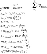
As stated in eq 17, the variables penalized from their optimal values are the reactor temperature and optimal decision variables given by the SDRTO layer, which correspond to molar flow rates of air, propylene, steam, and mass flow rate of the utility fluid. The tuning parameters used in the tracking objective function were Q1 = 1, R1 = 0.05, R2 = 0.05, R3 = 0.05, R4 = 0.05, P1 = 0.01, P2 = 0.01, P3 = 0.01, and P4 = 0.01.
For solving the stochastic dynamic optimization problems state in eqs 12 and 16, a sequential approach was implemented. The selected decision variables are discretized using eqs 8 and 9, and a metaheuristic algorithm (simulated annealing) is used for solving the resulting NLP problem. This stochastic algorithm does not need information about states derivatives, reducing computing time. Hybrid algorithms such as particle swarm optimization with genetic algorithms (PSO-GA),77 GA-GSA using uncertain data,78 and time-varying acceleration coefficient particle swarm, optimization with mutation strategies (TVAC-PSO-MS),79 could be also used for solving the resulting NLP problem.
The model of the process used in the SDRTO and multistage NMPC layers is solved in MATLAB using the stiff.Rosenbrock (ode 23 s) solver. The SDRTO layer model uses a prediction horizon of 2 h and is called when (i) a known disturbance occurs, (ii) there is deterioration in the economic objective function, and/or (iii) every 0.5 h. The multistage NMPC layer model uses a prediction horizon of 2 h and is called periodically every 0.2 h or when there is deterioration in the tracking objective function. Figure 4 shows the framework for the implemented stochastic multilayer strategy. Decision variables given by the solution of the optimization problem in the SDRTO layer are sent to the regulatory layer to satisfy optimal economic conditions for all of the scenarios. Decision variables given by the solution of the optimization problem in the NMPC layer are applied in the real plant.
Figure 4.

Stochastic multilayer strategy implemented in MATLAB.
3.4. Results
This section presents results for the acrylic acid reactor control problem under uncertainties. The problem is solved using a multilayer stochastic DyOP approach, and the results are compared against a single-layer stochastic DyOP approach (which uses simple PI control loops instead of a multistage NMPC in the regulatory layer), a deterministic DyOP approach that solved the DyOP problem using nominal values for uncertainty, and a typical simple PI control loop structure (shown in Figure 3). The simple PI control loop structure is composed of two PI controllers. The reactor temperature and pressure are selected as control objectives. The manipulated variables are the mass flow rate of the utility fluid in the jacket (ṁj) and the volumetric flow rate at the reactor output (q̇out). These local manipulated variables are calculated using the basic PI control laws shown in eqs 18 and 19
| 18 |
| 19 |
where Tsp and Pspare the respective
set-points. The tuning
parameters were obtained using the Ciancone correlations80 ,
,  ,
,  , and
, and  .
.
Tree layers compose the deterministic and multilayer stochastic DyOP approaches: an optimization layer, a regulatory layer, and the real plant. In the first, maximization of the economic profitability function (15) is carried out. The solution of this layer results in the calculation of the air molar flow rate (Fair), propylene molar flow rate (FC3H6), steam molar flow rate (Fsteam), the utility fluid mass flow rate (ṁj), and the optimal set-point value for the temperature (Tsp). The reactor temperature, deviations of decision variables around the references trajectories given by the DRTO layer, and penalizations in control movements for ensuring smooth operation are tracked by the NMPC controller. Optimal decision variable trajectories given by the NMPC are applied to the real plant. The deterministic DyOP approach does not consider uncertainty evolution. Therefore, the optimization problem is solved using nominal values for external and internal uncertainties. In the stochastic DyOP approach, the uncertainty evolution is modeled using the scenario tree representation shown in Figure 2. Three sources of uncertainties are evaluated to compare the tested approaches: variations in the acrylic acid price (external uncertainty), changes in the activation energy in the main reaction (internal uncertainty), and changes in the temperature of the air feed to the reactor (unknown disturbance). For simulation purposes, uncertainty is revealed after 0.4 h in the scenario tree for comparison of the four analyzed structures.
Figures 5–8 show results for simple PI control loops, deterministic DyOP, and single and multilayer stochastic DyOP approaches, when there is a model mismatch (variation in the activation energy). Figures 5 and 6 show results for the optimistic scenario; the minimum activation energy EA1 = 13927.02 kcal/kmol. This condition favors the reaction rate of the first reaction and disfavors the third reaction, increasing the acrylic acid production and leading the process to higher economic profitability. This condition also drives the reactor to a lower temperature by a decrease in carbon dioxide production. From Figure 6, we can observe that the stochastic multilayer DyOP approach reaches the highest economic profitability, with second place occupied by the single-layer stochastic DyOP approach, third place by the deterministic DyOP approach, and the last by the simple PI control loop structure. The optimal air/propylene molar flow rate ratio to maximize acrylic acid production was the strategy implemented for the multilayer stochastic approach to improve economic profitability. The simple PI control loop structure occupied the worst place since its unique objective is maintaining the control objectives at their set-points, without taking into account the profitability of the process. Good control performance is observed for the stochastic multilayer and the simple PI control loop structures, unlike for the stochastic single-layer and deterministic DyOP approaches, where the regulatory controller is unable of tracking adequately the reactor temperature trajectory. In the case of the deterministic DyOP approach, this behavior is caused by the inability of the optimizer for handling model mismatches, calculating inadequate decision variables as a consequence of considering nominal model parameters. For the stochastic single-layer structure, the inability of PI controllers is evident for tracking optimal trajectories given by the optimization layer, unlike when a multistage NMPC is used in the regulatory layer, which uses a rigorous dynamic nonlinear model of the process to predict its future behavior.
Figure 5.

Decision variable profiles for internal uncertainty; optimistic scenario EA1 = EA1min.
Figure 8.

Reactor temperature, the oxygen molar fraction, and economic profitability for internal uncertainty; pessimistic scenario EA1 = EA1max.
Figure 6.

Reactor temperature, the oxygen molar fraction inside the reactor, and economic profitability for internal uncertainty; optimistic scenario EA1 = EA1min.
A violation of the safety constraint (oxygen molar fraction in the reactor is higher than 5% after 4 h) took place for the deterministic DyOP approach, caused by inadequate calculation of optimal operation conditions by the optimizer. No constraint violation occurred in the simple PI control loops and stochastic approaches.
Figures 7 and 8 show the results for the pessimistic scenario; the maximum activation energy EA1 = 16072.967 kcal/kmol. The increase of activation energy for the main reaction reduces acrylic acid production and drives the process to lower economic profitability. This condition also produces a higher reactor temperature by increasing carbon dioxide production. From Figure 8, we can observe higher economic profitability for the stochastic multilayer DyOP approach, with the second place occupied by the stochastic single-layer approach, the third place occupied by the deterministic DyOP approach, and the worst behavior for the simple PI control loop structure. An increase in acrylic acid production by optimal air/propylene molar flow rate ratio was the strategy implemented by the multilayer stochastic approach for counteracting negative effects on the process profitability, caused by a higher value of activation energy. An increase in the steam flow rate was another strategy used by the stochastic approach to cool the reactor and favor acrylic acid production. Bad control performance was obtained for the simple PI control loop scheme, deterministic approach, and stochastic single-layer structure, unlike the multilayer stochastic approach where the multistage NMPC controller follows adequately the optimal temperature trajectory given by the optimization layer. No safety constraint violation occurs for any of the analyzed control structures.
Figure 7.

Decision variable profiles for internal uncertainty; pessimistic scenario EA1 = EA1max.
Table 4 shows the cumulative profitability comparison for internal uncertainty. For minimum and maximum values of activation energy, the stochastic multilayer approach reached higher profitability, showing its ability for counteracting internal uncertainty, driving the process to optimal economic conditions.
Table 4. Cumulative Profitability Comparison for Variation in the Activation Energy.
| tested architecture | cumulative profitability (USD) EA1min | cumulative profitability (USD) EA1max |
|---|---|---|
| simple PI control loops | –1.2177 × 10⁵ | –1.5121 × 10⁴ |
| deterministic DyOP approach | –1.2780 × 10⁵ | –2.4394 × 10⁴ |
| stochastic DyOP approach (two layer) | –1.3659 × 10⁵ | –2.7838 × 10⁴ |
| stochastic DyOP approach (one layer) | –1.3348 × 10⁵ | –2.5837 × 10⁴ |
Table 5 shows the CPU time required for solving the stochastic and deterministic approaches. All proposed optimization problems were solved in MATLAB on a standard Asus laptop with an Intel i-7 processor at 2.59 GHz with four cores and 8 GB of RAM. Higher computing time is obtained by the multilayer stochastic approach since a robust solution of the DyOP implies increasing its mathematical complexity with higher computing demands. Table 6 shows the CPU time required for solving optimization problems in upper and regulatory layers for multilayer stochastic optimization. The calculation optimization time for the upper layer is higher than the regulatory layer due to the higher complexity of the economic objective function with respect to the tracking objective function used in the regulation layer.
Table 5. CPU Time Comparison for the Internal Uncertainty Case.
| tested architecture | simulation time (h) |
|---|---|
| deterministic approach | 0.159 |
| stochastic single-layer approach | 0.264 |
| stochastic multilayer approach | 0.448 |
Table 6. CPU Time Comparison for the Multilayer Stochastic Approach.
| tested architecture | simulation time (h) |
|---|---|
| economic layer | 0.259 |
| regulatory layer | 0.189 |
Figures 9–12 show results for simple PI control loops, deterministic, and stochastic approaches, when there is an external uncertainty (variation in the acrylic acid price). Figures 9 and 10 show results for the minimum acrylic acid price (AAprice = 121.233 USD/kmol). In this pessimistic scenario, the acrylic acid price is lower than the nominal value, which reduces considerably the economic profitability of the process and it can make it unprofitable. From Figure 10, we can observe higher economic profitability reached by the multilayer stochastic approach, with second place occupied by the single-layer stochastic approach, third place occupied by the deterministic approach, and the last place by the simple PI control loop structure. The strategy implemented by the stochastic multilayer approach consisted of obtaining an optimal air/propylene molar flow rate ratio to increase acrylic acid production. The reduction in propylene and steam molar flow rates was another strategy used by the stochastic multilayer approach to decrease the cost of raw materials and therefore improve the process profitability. The strategy used by the deterministic approach corresponds to the nominal operation, which leads the process toward a conservative solution. The simple PI control loop structure does not consider process profitability, and therefore, results in the worst economic operation. Good control performance and constraint fulfillments are observed in Figure 10 for all of the analyzed structures.
Figure 9.

Decision variable profiles for external uncertainty; pessimistic scenario cAA = cAA min.
Figure 12.

Reactor temperature, the oxygen molar fraction, and economic profitability for external uncertainty; optimistic scenario cAA = cAA max.
Figure 10.

Reactor temperature, the oxygen molar fraction, and economic profitability for external uncertainty; pessimistic scenario cAA = cAA min.
Figures 11 and 12 show the results for the maximum acrylic acid price (AAprice = 225.147 USD/kmol). In this optimistic scenario, the acrylic acid price is higher than the nominal value, and the economic profitability increases for all of the analyzed control structures. The stochastic multilayer scheme reaches the best economic profitability, followed by the stochastic single-layer structure; the third place is occupied by the deterministic approach and the last place by the simple PI control loop structure. An increase in the air molar flow rate and a reduction in propylene and steam molar flow rates to improve acrylic acid production and reduce the cost of raw materials is the strategy employed by the stochastic multilayer approach to maximize process profitability. Good control performance and fulfillment of constraints for all control structures are observed in Figure 12. The above allows one to conclude that, unlike internal uncertainties (model mismatches), external uncertainties do not greatly affect the control performance of the stochastic single layer, simple PI, and deterministic approaches.
Figure 11.

Decision variable profiles for external uncertainty; optimistic scenario cAA = cAA max.
Table 7 shows the cumulative profitability for uncertain market conditions. The stochastic multilayer scheme reaches the best economic profitability, followed by the stochastic single-layer structure. The deterministic and simple PI control loop structures do not react to adverse price scenarios of acrylic acid, and therefore, they are not recommended for handling cost marketing uncertainties.
Table 7. Cumulative Profitability Comparison for Changes in the Acrylic Acid Price.
| tested architecture | cumulative profitability (USD): lower AAprice | cumulative profitability (USD): higher AAprice |
|---|---|---|
| simple PI control loops | –4.5667 × 10⁴ | –1.4024 × 10⁵ |
| deterministic DyOP approach | –5.1085 × 10⁴ | –1.4940 × 10⁵ |
| stochastic DyOP approach (two layer) | –5.1746 × 10⁴ | –1.5033 × 10⁵ |
| stochastic DyOP approach (one layer) | –5.1255 × 10⁴ | –1.4933 × 10⁵ |
Table 8 shows the total simulation time for market uncertainty evaluation. A higher computing time was obtained for the stochastic multilayer approach since it evaluates different values of uncertainty market conditions and solves two optimization problems in both layers.
Table 8. CPU Time Comparison for the External Uncertainty Case.
| tested architecture | simulation time (h) |
|---|---|
| deterministic approach | 0.128 |
| stochastic single-layer approach | 0.216 |
| stochastic multilayer approach | 0.392 |
Figures 13 and 14 present results for single and multilayer stochastic approaches, when there is an unknown process uncertainty. Changes in the air temperature during the control experiment according to its PDF have been implemented for comparison of both structures. Higher economic profitability and best control performance are obtained by the multilayer stochastic approach. These results show the robustness of the stochastic multilayer approach to reject unknown process disturbances, driving the process to a viable operation from an economical and control point of view. A higher simulation time is obtained by the stochastic multilayer approach (see Table 9) since the presence of a multistage NMPC in the regulatory layer implies a higher mathematical complexity of the problem.
Figure 13.

Decision variables for the unknown process uncertainty.
Figure 14.

Reactor temperature, the oxygen molar fraction, and economic profitability for the unknown process uncertainty.
Table 9. CPU Time Comparison for the Unknown Process Uncertainty Case.
| tested architecture | simulation time (h) |
|---|---|
| single-layer approach | 0.228 |
| multilayer approach | 0.319 |
Figures 15 and 16 present the results for single and multilayer stochastic approaches, with Monte Carlo simulations in internal and external uncertainties. Random behaviors of the activation energy and acrylic acid cost acting at the same time have been implemented for the comparison of both structures. Three scenarios are evaluated randomly from PDF of internal uncertainties and market conditions: scenario 1 = {16781.50; 145.6141}, scenario 2 = {14868; 124.0237}, and scenario 3 = {15564.56; 207.3130}. Higher economic profitability and best control performance are obtained by the multilayer stochastic approach. Figure 16 shows the inability of the stochastic single-layer structure for tracking optimal state trajectories given by the optimization layer. For these reasons, the stochastic multilayer approach is preferred.
Figure 15.

Economic profitability for the uncertainty Monte Carlo simulations.
Figure 16.

Reactor temperature for the uncertainty Monte Carlo simulations.
Finally, a Student’s t-test was performed to obtain economic profitability values (objective function) for stochastic, deterministic, and simple PI approaches for internal uncertainty.
Comparing the stochastic multilayer and deterministic DyOP approaches, the p-value obtained was 6.79732 × 10⁻⁵, which indicates that the difference between these objective functions is significant, thus showing a considerable improvement in terms of profitability when the stochastic multilayer strategy is implemented. Similar results were obtained when the stochastic multilayer approach was compared against the simple PI control. In this case, the p-value obtained was 9.20997 × 10⁻⁹.
4. Conclusions
The proposal of a multilayer stochastic optimization approach for handling different sources of uncertainties (model mismatches, market conditions, and unknown process disturbances) was presented. The potential of the proposed approach was proved by simulation in a CSTR reactor for acrylic acid production. The performance of the proposed approach to deal with different sources of uncertainties is compared with a simple PI control loop structure, a deterministic DyOP approach, and a stochastic single-layer structure. Simulation results show that the multilayer stochastic optimization approach improves economic profitability, with a good performance of the control system for tracking state trajectories and satisfactory safety constraints for all of the scenarios considered. The stochastic single-layer approach occupied second place in terms of economic profitability; however, as its objective is purely economic it does not track the optimal state trajectories. The deterministic DyOP approach occupied third place in economic profitability and does not show good control performance and satisfactory safety constraints for internal uncertainties. The simple PI control loop structure showed the worst values for the economic profitability in the presence of uncertainties
The main drawback of the proposed multilayer stochastic optimization approach is the increased computing time. The presence of many uncertain variables in the plant or considering a scenario tree with many stages could be a limitation for this structure since the DRTO problem could be intractable.
Future work includes formulating a parallelized decomposition version of the multilayer stochastic optimization approach for parallel computing implementation for the sake of reducing computing time and implementation costs. The extension of the proposed approach for handling uncertainties and solving the stochastic DyOP for a complete process plant is another subject for future work. The development of strategies for plantwide optimizing control (PWOC) in the presence of uncertainties is mandatory for large-scale industrial purposes.
Acknowledgments
Andrés Duque thanks the economic support received from the Colombian Ministry of Science, Technology and Innovation and Sapiencia under the scholarships “Doctorados Nacionales-647” and “Enlaza mundos-2018”.
A. Process Model
For handling uncertainties from a dynamic optimization point of view, a rigorous nonlinear dynamic model of the process is necessary. This model is essential to predict future process operations and evaluate uncertainty evolution. For modeling acrylic acid reactor, mass and energy conservation equations are applied in a transient state. The total mass balance in the reactor is given by eqs A1–A3
| A1 |
| A2 |
| A3 |
where Ḟin are the inlet molar flow rates of air, propylene, and steam, Ḟout is the total molar flow rate coming out the reactor, Ṙgen is the total reaction rate, and n, R, V, P, and T are the total moles, universal gas constant, volume, pressure, and reactor temperature, respectively. Molar balances by components are given by eqs A4–A6
| A4 |
| A5 |
| A6 |
where Cj are the molar species concentration in the reactor (j = AA, O2, ACE, C3H6, H2O, CO2, N2), qinCjin is the total molar flow rate of species j entering the reactor, qoutCj is the total molar flow rate of species j leaving the reactor, vij are stoichiometric coefficients for species j at reaction i, ri is the specific reaction rate for reaction i, and ns is the number of reactions in the model. Energy balances inside the reactor and for the utility fluid in the jacket are given by eqs A7 and A8
| A7 |
| A8 |
where m is the total mass in the reactor, cv is the average specific heat of the mixture inside the reactor, Ḟjin is the total molar flow rate of species j at the reactor inlet, Ḟout is the total molar flow rate of species j at the reactor outlet, hjin and hout are molar enthalpies of feed and outlet streams, respectively, ΔHRi is the heat of each reaction i. ρJ, CvJ, ṁJ, CpJ are the density, specific heat at constant volume, mass flowrate, and specific heat at constant pressure for the utility fluid (cooling water) respectively. VJ, At, and U are the volume of the jacket, heat transfer area, and global coefficient of heat transfer, respectively. Finally, T andTJ are the reactor and utility fluid temperatures. Figure 3 is a schematic representation of the reactor.
The authors declare no competing financial interest.
References
- French M.Optimization: The Big Idea. In Fundamentals of Optimization; Springer International Publishing, 2018; pp 1–13. [Google Scholar]
- French M.Getting Started in Optimization: Problems of a Single Variable. In Fundamentals of Optimization; Springer International Publishing, 2018; pp 15–54. [Google Scholar]
- Butenko S.; Pardalos P. M.. Numerical Methods and Optimization: An Introduction. In Numerical Methods and Optimization; Chapman and Hall/CRC, 2014. [Google Scholar]
- Arellano-garcia H.Chance Constrained Optimization of Process Systems under Uncertainty. Doctoral Thesis, Technische Universität Berlin: Berlín, 2006. [Google Scholar]
- Beale E. M. L. Linear Programming under Uncertainty. J. R. Stat. Soc., Ser. B 1955, 17, 173–184. [Google Scholar]
- Dantzig G. B. Linear Programming under Uncertainty. Manage. Sci. 1955, 1, 197–206. 10.1287/mnsc.1.3-4.197. [DOI] [Google Scholar]
- Pistikopoulos E. N.; Ierapetritou M. G. Novel Approach for Optimal Process Design under Uncertainty. Comput. Chem. Eng. 1995, 19, 1089–1110. 10.1016/0098-1354(94)00093-4. [DOI] [Google Scholar]
- Rooney W. C.; Biegler L. T. Incorporating Joint Confidence Regions into Design under Uncertainty. Comput. Chem. Eng. 1999, 23, 1563–1575. 10.1016/S0098-1354(99)00311-7. [DOI] [Google Scholar]
- Rooney W. C.; Biegler L. T. Design for Model Parameter Uncertainty Using Nonlinear Confidence Regions. AIChE J. 2001, 47, 1794–1804. 10.1002/aic.690470811. [DOI] [Google Scholar]
- Rooney W. C.; Biegler L. T. Optimal Process Design with Model Parameter Uncertainty and Process Variability. AIChE J. 2003, 49, 438–449. 10.1002/aic.690490214. [DOI] [Google Scholar]
- Shi H.; You F. A Computational Framework and Solution Algorithms for Two-Stage Adaptive Robust Scheduling of Batch Manufacturing Processes under Uncertainty. AIChE J. 2016, 62, 687–703. 10.1002/aic.15067. [DOI] [Google Scholar]
- Gong J.; Garcia D. J.; You F. Unraveling Optimal Biomass Processing Routes from Bioconversion Product and Process Networks under Uncertainty: An Adaptive Robust Optimization Approach. ACS Sustainable Chem. Eng. 2016, 4, 3160–3173. 10.1021/acssuschemeng.6b00188. [DOI] [Google Scholar]
- Lappas N. H.; Gounaris C. E. Multi-Stage Adjustable Robust Optimization for Process Scheduling under Uncertainty. AIChE J. 2016, 62, 1646–1667. 10.1002/aic.15183. [DOI] [Google Scholar]
- Gong J.; You F. Optimal Processing Network Design under Uncertainty for Producing Fuels and Value-Added Bioproducts from Microalgae: Two-Stage Adaptive Robust Mixed Integer Fractional Programming Model and Computationally Efficient Solution Algorithm. AIChE J. 2017, 63, 582–600. 10.1002/aic.15370. [DOI] [Google Scholar]
- Charnes A.; Cooper W. W. Chance-Constrained Programming. Manage. Sci. 1959, 6, 73–79. 10.1287/mnsc.6.1.73. [DOI] [Google Scholar]
- Arellano-Garcia H.; Martini W.; Wendt M.; Wozny G. In Chance Constrained Batch Distillation Process Optimization under Uncertainty, Proceedings of the International Conference on Foundations of Computer-Aided Process Operations, 2003; pp 609–612.
- Geletu A.; Klöppel M.; Zhang H.; Li P. Advances and Applications of Chance-Constrained Approaches to Systems Optimisation under Uncertainty. Int. J. Syst. Sci. 2013, 44, 1209–1232. 10.1080/00207721.2012.670310. [DOI] [Google Scholar]
- Geletu A.; Li P. Recent Developments in Computational Approaches to Optimization under Uncertainty and Application in Process Systems Engineering. ChemBioEng Rev. 2014, 1, 170–190. 10.1002/cben.201400013. [DOI] [Google Scholar]
- Henrion R.; Möller A. Optimization of a Continuous Distillation Process under Random Inflow Rate. Comput. Math. Appl. 2003, 45, 247–262. 10.1016/S0898-1221(03)80017-2. [DOI] [Google Scholar]
- Li P.; Wendt M.; Wozny G. Optimal Production Planning for Chemical Processes under Uncertain Market Conditions. Chem. Eng. Technol. 2004, 27, 641–651. 10.1002/ceat.200400048. [DOI] [Google Scholar]
- Li P.; Wendt M.; Wozny G. A Probabilistically Constrained Model Predictive Controller. Automatica 2002, 38, 1171–1176. 10.1016/S0005-1098(02)00002-X. [DOI] [Google Scholar]
- Li P.; Wendt M.; Wozny G. Robust Model Predictive Control under Chance Constraints. Comput. Chem. Eng. 2000, 24, 829–834. 10.1016/S0098-1354(00)00398-7. [DOI] [Google Scholar]
- Müller D.; Illner M.; Esche E.; Pogrzeba T.; Schmidt M.; Schomäcker R.; Biegler L. T.; Wozny G.; Repke J.-U. Dynamic Real-Time Optimization under Uncertainty of a Hydroformylation Mini-Plant. Comput. Chem. Eng. 2017, 106, 836–848. 10.1016/J.COMPCHEMENG.2017.01.041. [DOI] [Google Scholar]
- Müller D.; Esche E.; Werk S.; Wozny G. Dynamic Chance-Constrained Optimization under Uncertainty on Reduced Parameter Sets. Comput.-Aided Chem. Eng. 2015, 37, 725–730. 10.1016/B978-0-444-63578-5.50116-X. [DOI] [Google Scholar]
- Verderame P. M.; Floudas C. A. Operational Planning of Large-Scale Industrial Batch Plants under Demand Due Date and Amount Uncertainty. I. Robust Optimization Framework. Ind. Eng. Chem. Res. 2009, 48, 7214–7231. 10.1021/ie9001124. [DOI] [Google Scholar]
- Wendt M.; Li P. Nonlinear Chance-Constrained Process Optimization under Uncertainty. Ind. Eng. Chem. Res. 2002, 41, 3621–3629. 10.1021/ie010649s. [DOI] [Google Scholar]
- Raff T.; Ebenbauer C.; Allgöwer F.. Nonlinear Model Predictive Control: A Passivity-Based Approach. In Assessment and Future Directions of Nonlinear Model Predictive Control; Springer: Berlin, Heidelberg, 2007; Vol. 358. [Google Scholar]
- Campo P. J.; Morari M. In Robust Model Predictive Control, American Control Conference; IEEE, 1987; pp 1021–1026.
- Schwarm A. T.; Nikolaou M. Chance-Constrained Model Predictive Control. AIChE J. 1999, 45, 1743–1752. 10.1002/aic.690450811. [DOI] [Google Scholar]
- Li P.; Wendt M.; Wozny G. A Probabilistically Constrained Model Predictive Controller. Automatica 2002, 38, 1171–1176. 10.1016/S0005-1098(02)00002-X. [DOI] [Google Scholar]
- Schwarm A.; Nikolaou M. Chance-Constrained Model Predictive Control. AIChE J. 1999, 45, 1743–1752. 10.1002/aic.690450811. [DOI] [Google Scholar]
- Hessem D. H. V.; Bosgra O. H. In A Full Solution to the Constrained Stochastic Closed-Loop MPC Problem via State and Innovations Feedback and Its Receding Horizon Implementation, Proceedings of the 42nd IEEE Conference on Decision and Control; Maui, 2003; pp 929–934.
- Kim K. K.; Braatz R. D. In Generalized Polynomial Chaos Expansion Approaches to Approximate Stochastic Receding Horizon Control with Applications to Probabilistic Collision Checking and Avoidance, Proceedings of the IEEE International Conference on Control Applications; Dubrovnik, 2012; pp 350–355.
- Vidyasagar M. Randomized Algorithms for Robust Controller Synthesis Using Statistical Learning Theory. Automatica 2000, 37, 1515–1528. 10.1016/S0005-1098(01)00122-4. [DOI] [Google Scholar]
- Shapiro A. Stochastic Programming Approach to Optimization under Uncertainty. Math. Program. 2008, 12, 182–220. 10.1007/s10107-006-0090-4. [DOI] [Google Scholar]
- Calafiore G. C.; Fagiano L. Robust Model Predictive Control via Scenario Optimization. IEEE Trans. Autom. Control 2013, 58, 219–224. 10.1109/TAC.2012.2203054. [DOI] [Google Scholar]
- Zhang X.; Margellos K.; Goulart P.; Lygeros J. In Stochastic Model Predictive Control Using a Combination of Randomized and Robust Optimization, Proceedings of the 52nd IEEE Conference on Decision and Control; Florence, 2013; pp 7740–7745.
- Wiener N. The Homogeneous Chaos. Am. J. Math. 1938, 60, 897–936. 10.2307/2371268. [DOI] [Google Scholar]
- Ghanem R.; Spanos P.. Stochastic Finite Elements—A Spectral Approach; Springer-Verlag: New York, 1991. [Google Scholar]
- Xiu D.; Karniadakis G. E. The Wiener-Askey Polynomial Chaos for Stochastic Differential Equations. SIAM J. Sci. Comput. 2002, 24, 619–644. 10.1137/S1064827501387826. [DOI] [Google Scholar]
- Hover F. S.; Triantafyllou M. S. Application of Polynomial Chaos in Stability and Control. Automatica 2006, 42, 789–795. 10.1016/j.automatica.2006.01.010. [DOI] [Google Scholar]
- Nagy Z. K.; Braatz R. D. Distributional Uncertainty Analysis Using Power Series and Polynomial Chaos Expansions. J. Process Control 2007, 17, 229–240. 10.1016/j.jprocont.2006.10.008. [DOI] [Google Scholar]
- Fisher J.; Bhattacharya R. Linear Quadratic Regulation of Systems with Stochastic Parameter Uncertainties. Automatica 2011, 45, 2831–2841. 10.1016/j.automatica.2009.10.001. [DOI] [Google Scholar]
- Fisher J.; Bhattacharya R. Optimal Trajectory Generation with Probabilistic System Uncertainty Using Polynomial Chaos. J. Dyn. Syst., Meas., Control 2011, 133, 014501 10.1115/1.4002705. [DOI] [Google Scholar]
- Fagiano L.; Khammash M. In Nonlinear Stochastic Model Predictive Control via Regularized Polynomial Chaos Expansions, Proceedings of the 51st IEEE Conference on Decision and Control; Maui, 2012; pp 142–147.
- Mesbah A.; Streif S.; Findeisen R.; Braatz R. D. In Stochastic Nonlinear Model Predictive Control with Probabilistic Constraints, 2014 American Control Conference (ACC); Portland, Oregon, USA, 2014; pp 2413–2419.
- Fagiano L.; Khammash M. In Nonlinear Stochastic Model Predictive Control via Regularized Polynomial Chaos Expansions, 2012 IEEE 51st IEEE Conference on Decision and Control (CDC), 2012; pp 142–147.
- Paulson J. A.; Buehler E. A.; Braatz R. D.; Mesbah A. Stochastic Model Predictive Control with Joint Chance Constraints. Int. J. Control 2020, 93, 126–139. 10.1080/00207179.2017.1323351. [DOI] [Google Scholar]
- Mesbah A. Stochastic Model Predictive Control: An Overview and Perspectives for Future Research. IEEE Control Syst. Mag. 2016, 36, 30–44. 10.1109/MCS.2016.2602087. [DOI] [Google Scholar]
- Paulson J. A.; Mesbah A. An Efficient Method for Stochastic Optimal Control with Joint Chance Constraints for Nonlinear Systems. Int. J. Robust Nonlinear Control 2019, 29, 5017–5037. 10.1002/rnc.3999. [DOI] [Google Scholar]
- Lucia S.; Finkler T.; Engell S. Multi-Stage Nonlinear Model Predictive Control Applied to a Semi-Batch Polymerization Reactor under Uncertainty. J. Process Control 2013, 23, 1306–1319. 10.1016/j.jprocont.2013.08.008. [DOI] [Google Scholar]
- Lucia S.; Andersson J. A. E.; Brandt H.; Diehl M.; Engell S. Handling Uncertainty in Economic Nonlinear Model Predictive Control: A Comparative Case Study. J. Process Control 2014, 24, 1247–1259. 10.1016/j.jprocont.2014.05.008. [DOI] [Google Scholar]
- Yu Z. J.; Biegler L. T.. Advanced-Step Multistage Nonlinear Model Predictive Control; IFAC-PapersOnLine, 2018; Vol. 51, pp 122–127. [Google Scholar]
- Engell S. In Online Optimizing Control: The Link between Plant Economics and Process Control, Computer Aided Chemical Engineering, 10th International Symposium on Process Systems Engineering; Elsevier B.V, 2009; pp 79–86.
- Suo X.; Zhang H.; Ye Q.; Dai X.; Yu H.; Li R. Design and Control of an Improved Acrylic Acid Process. Chem. Eng. Res. Des. 2015, 104, 346–356. 10.1016/j.cherd.2015.08.022. [DOI] [Google Scholar]
- Luyben W. L. Economic Trade-Offs in Acrylic Acid Reactor Design. Comput. Chem. Eng. 2016, 93, 118–127. 10.1016/j.compchemeng.2016.06.005. [DOI] [Google Scholar]
- Duque A.; Ochoa S. In A Comparison of Control Architectures for Controlling a CSTR for Acrylic Acid Production, 2019 IEEE 4th Colombian Conference on Automatic Control (CCAC), 2019; pp 1–6.
- Müller D.Development of Operation Trajectories Under Uncertainty for a Hydroformylation Mini-Plant; Technische Universität Berlin, 2015. [Google Scholar]
- Louveaux F.; Birge J. R.. Introduction to Stochastic Programming, 2nd ed.; Springer: New York, 2011. [Google Scholar]
- Navia D.; Sarabia D.; Gutiérrez G.; Cubillos F.; de Prada C. A Comparison between Two Methods of Stochastic Optimization for a Dynamic Hydrogen Consuming Plant. Comput. Chem. Eng. 2014, 63, 219–233. 10.1016/j.compchemeng.2014.02.004. [DOI] [Google Scholar]
- Dupacova J. Multistage Stochastic Programs—the State-of-the-Art and Selected Bibliography. Kybernetika 1995, 31, 151–174. 10.1039/c4nr04226c. [DOI] [Google Scholar]
- Dupačová J.; Dupačová D.; Wallace S. W. Scenarios for Multistage Stochastic Programs. Ann. Oper. Res. 2000, 100, 25–53. 10.1023/A:1019206915174. [DOI] [Google Scholar]
- Sahinidis N. V. Optimization under Uncertainty: State-of-the-Art and Opportunities. Comput. Chem. Eng. 2004, 28, 971–983. 10.1016/j.compchemeng.2003.09.017. [DOI] [Google Scholar]
- Mayne D. Q.; Seron M. M.; Raković S. V. Robust Model Predictive Control of Constrained Linear Systems with Bounded Disturbances. Automatica 2005, 41, 219–224. 10.1016/j.automatica.2004.08.019. [DOI] [Google Scholar]
- Mayne D. Q.; Kerrigan E. C.; van Wyk E. J.; Falugi P. Tube-Based Robust Nonlinear Model Predictive Control. Int. J. Robust Nonlinear Control 2011, 21, 1341–1353. 10.1002/rnc.1758. [DOI] [Google Scholar]
- Rawlings J.; Mayne D.. Model Predictive Control Theory and Design; Nob Hill Publishing: Madison, WI, 2009. [Google Scholar]
- Mayne D. Q.; Kerrigan E. C.; Falugi P. In Robust Model Predictive Control: Advantages and Disadvantages of Tube-Based Methods; IFAC Proceedings Volumes (IFAC-PapersOnline); IFAC Secretariat, 2011; Vol. 44, pp 191–196. [Google Scholar]
- Raković S. V.; Kouvaritakis B.; Cannon M.; Panos C.; Findeisen R. In Fully Parameterized Tube MPC; IFAC Proceedings Volumes (IFAC-PapersOnline); IFAC Secretariat, 2011; Vol. 44, pp 197–202. [Google Scholar]
- Yu S.; Chen H.; Allgower F. In Tube MPC Scheme Based on Robust Control Invariant Set with Application to Lipschitz Nonlinear Systems, Proceedings of the IEEE Conference on Decision and Control, 2011; pp 2650–2655.
- Ochoa S.Plantwide Optimizing Control for the Continuous Bio-Ethanol Production Process. Ph.D. Dissertation, TU Berlin: Berlin, 2010. [Google Scholar]
- Lucia S.Robust Multi-Stage Nonlinear Model Predictive Control; Shaker: Dortmund, 2015. [Google Scholar]
- Lange J. P.Production of Acrylic Acid. U.S. Patent US201503534652016.
- Turton R.; Bailie R. C.; Whiting W. B.; Shaeiwitz J. A.; Bhattacharyya D.. Analysis, Synthesis, and Design of Chemical Processes; Prentice Hall: New York, 2012. [Google Scholar]
- Carlson E. C. Don’t Gamble With Physical Properties. Chem. Eng. Prog. 1996, 35–46. [Google Scholar]
- Ganzer G.; Freund H. Kinetic Modeling of the Partial Oxidation of Propylene to Acrolein: A Systematic Procedure for Parameter Estimation Based on Non-Isothermal Data. Ind. Eng. Chem. Res. 2019, 58, 1857–1874. 10.1021/acs.iecr.8b05583. [DOI] [Google Scholar]
- ICIS.com. Work for ICIS, 2021. https://www.icis.com/explore/.
- Garg H. A Hybrid PSO-GA Algorithm for Constrained Optimization Problems. Appl. Math. Comput. 2016, 274, 292–305. 10.1016/j.amc.2015.11.001. [DOI] [Google Scholar]
- Garg H.A Hybrid GA-GSA Algorithm for Optimizing the Performance of an Industrial System by Utilizing Uncertain Data. In Handbook of Research on Artificial Intelligence Techniques and Algorithms; IGI Global, 2014; pp 620–654. [Google Scholar]
- Patwal R. S.; Narang N.; Garg H. A Novel TVAC-PSO Based Mutation Strategies Algorithm for Generation Scheduling of Pumped Storage Hydrothermal System Incorporating Solar Units. Energy 2018, 142, 822–837. 10.1016/j.energy.2017.10.052. [DOI] [Google Scholar]
- Marlin T. E.Process Control: Designing Processes and Control Systems for Dynamic Performance; McGraw-Hill, 2000. [Google Scholar]