Identifiability of Tissue Material Parameters from Uniaxial Tests using Multi-start Optimization

Abstract

Determining tissue biomechanical material properties from mechanical test data is frequently required in a variety of applications. However, the validity of the resulting constitutive model parameters is the subject of debate in the field. Parameter optimization in tissue mechanics often comes down to the “identifiability” or “uniqueness” of constitutive model parameters; however, despite advances in formulating complex constitutive relations and many classic and creative curve-fitting approaches, there is currently no accessible framework to study the identifiability of tissue material parameters. Our objective was to assess the identifiability of material parameters for established constitutive models of fiber-reinforced soft tissues, biomaterials, and tissue-engineered constructs and establish a generalizable procedure for other applications. To do so, we generated synthetic experimental data by simulating uniaxial tension and compression tests, commonly used in biomechanics. We then fit this data using a multi-start optimization technique based on the nonlinear least-squares method with multiple initial parameter guesses. We considered tendon and sclera as example tissues, using constitutive models that describe these fiber-reinforced tissues. We demonstrated that not all the model parameters of these constitutive models were identifiable from uniaxial mechanical tests, despite achieving virtually identical fits to the stress-stretch response. We further show that when the lateral strain was considered as an additional fitting criterion, more parameters are identifiable, but some remain unidentified. This work provides a practical approach for addressing parameter identifiability in tissue mechanics.

1. Introduction

Knowledge of material properties is valuable to study complex physiomechanical tissue function, to monitor pathophysiological changes, and to characterize tissue-engineered constructs [1]–[5]. Despite the widespread use of parameter optimization when fitting experimental data, there are important limitations to this technique arising from the uniqueness (or lack thereof) of the fitted parameters. The lack of uniqueness is problematic because it hinders the ability to measure a tissue’s mechanical properties and limits the usefulness of the measured in finite element modeling and other applications. Therefore, a systematic and practical understanding of this limitation in parameter optimization is needed.

Several optimization approaches have been used in tissue mechanics, yet their success is a subject of debate. Nonlinear least-squares optimization (NLSQ) is perhaps the most commonly used approach. However, NLSQ methods are prone to local minima traps and depend strongly on the initial guesses used in the fitting algorithm; further, when fitting parameters of highly complex, nonlinear, and anisotropic tissues, uniqueness (or identifiability) is another hurdle [6]. These problems limit the value of the resulting fitted parameters. Global optimization algorithms, such as genetic algorithms, particle swarm, and simulated annealing, have been used in tissue mechanics to avoid local minima trap with variable success [5], [7], [8].

Parameter optimization in tissue mechanics is often a problem in the “identifiability” or “uniqueness” of constitutive model parameters [9], [10]. A general definition for identifiability is provided in the classic text by Walter and Pronzato [10]. Several studies have previously addressed the identifiability of tissue material parameters. For example, Hartmann and Gilbert used the determinant of the Hessian matrix to study identifiability of the two parameters (bulk and shear modulus) describing an elastic material using analytical and finite element solutions [11]; in another study, Akintunde and co-workers used rank deficiency of the Fisher information matrix to study uncertainty and identifiability in murine patellar tendon stress-strain responses [12]. Several other studies have also addressed aspects of characterization of material parameters by using both phenomenological [13], [14], and micromechanical [15] modeling approaches. However, despite advances in formulating complex constitutive relations and curve-fitting approaches, there is currently no accessible framework to assess the identifiability of tissue material parameters.

The objective of this study was to assess the identifiability of material parameters for established constitutive models used to describe the anisotropic and nonlinear response of fiber-reinforced soft tissues, biomaterials, and tissue engineered constructs and establish a generalizable procedure for other applications. We used a numerical approach and focused on several commonly-performed canonical experiments: uniaxial tension and unconfined compression. We used a Monte-Carlo-type multi-start optimization approach [16], [17] that Safa and co-workers recently implemented to study poroelasticity and inelasticity of tendon [18], [19]. This method enables exploration of the search space around the initial guess and reveals parameter sets that produce the same mechanical response. We show that while some parameters are identifiable, many are not, even though nearly perfect fits to the stress-stretch response can be achieved. We further show that when we impose a second fitting criterion, namely lateral strain, more parameters are identifiable, but some are still not.

2. Methods

2.1. Overview

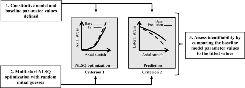
An overview of the methods is shown in Figure 1. We first specified constitutive models for nonlinear isotropic and fiber-reinforced anisotropic materials (Section 2.2, Table 1). We numerically implemented these models using the kinematics of uniaxial tension and compression with traction-free lateral boundary conditions (Section 2.3). We next used representative baseline material parameters from sclera in compression and tendon in tension to simulate the baseline “experimental” tissue stress-stretch data for each constitutive model (Section 2.4, Table 1). We then used a multi-start least-squares optimization curve-fit to the baseline response with a wide search space and 600 random initial guesses per material parameter and assessed the quality of the fits compared to the baseline stress-stretch response (Section 2.5). Because we observed that several parameter sets could reproduce the stress-stretch response, we added a second assessment criterion based on the quality of the lateral strain prediction (Section 2.6). Finally, we assessed the identifiability of each material parameter for each constitutive model by comparing the fitted parameter values to the baseline parameter values (Section 2.7).

Figure 1:

Schematic overview of the methods to assess the identifiability of model parameters. Briefly, (1) after implementing the constitutive models and selecting the baseline parameters based on the literature, (2) we conducted a multi-start nonlinear least squares (NLSQ) optimization by using randomly generated initial guesses; (3) we then assessed identifiability of the material parameters using two criteria, one based on the quality of the fit of axial stress (Criterion 1), and the other based on the prediction of the lateral strain (Criterion 2).

Table 1:

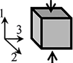
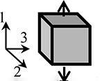
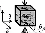
Summary of the model parameters, including baseline parameter values and ranges. In each model, the moduli are non-dimensionalized by normalizing with the corresponding matrix modulus.

Model		Matrix			Fibers
Isotropic Compression (IsoComp)		Neo Hookean			N/A
		ENH	νNH
	Base	1	0.3
	Min.	0	0
	Max.	10	0.45
Isotropic Tension (IsoTens)		Holmes-Mow
		EHM	νHM	βHM
	Base	1	0.3	5
	Min.	0	0	0
	Max.	10	0.45	60
Trans. Isotropic Compression (XIsoComp)		Neo Hookean			Uniform Distribution of Toe-linear Fibers				Fiber Direction
		ENH	νNH		Ef	βf	λ0	kVM
	Base	1	0.3		100	10	1.03	0	Distributed in the 2–3 plane around x2
	Min.	0	0		0	2	1	0
	Max.	10	0.45		1000	100	1.1	0
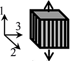
Trans. Isotropic Tension (XIsoTens)		Holmes-Mow			Aligned Toe-linear Fibers				Fiber Direction
		EHM	νHM	βHM	Ef	βf	λ0
	Base	1	0.3	5	200	10	1.03		x1
	Min.	0	0	0	0	2	1
	Max.	10	0.45	60	500	50	1.1
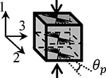
Orthotropic Compression (OrthoComp)		Neo Hookean			Non-uniform Distribution of Toe-linear Fibers				Fiber Direction
		ENH	νNH		Ef	βf	λ0	kVM
	Base	1	0.3		100	10	1.03	3	Distributed in 2–3 plane around x2
	Min.	0	0		0	2	1	0
	Max.	10	0.45		1000	100	1.1	5

2.2. Constitutive Models

Constitutive models for nonlinear isotropic and fiber-reinforced anisotropic materials that are loaded in uniaxial tension or compression were taken from well-established models [20]–[25]. We specifically considered two isotropic material models: neo-Hookean in compression and Holmes-Mow in tension, based on typical usage. We added fibers to these isotropic materials to achieve transverse isotropy or orthotropy. The constitutive models, derived from the Helmholtz free energy, are provided in Appendix A. The material parameters are briefly described below.

2.2.1. Isotropic models

For the isotropic model in compression (IsoComp), we used a compressible neo-Hookean material description [24], with the subscript “NH” being used throughout to refer to the neo-Hookean constitutive material parameters. The neo-Hookean constitutive relation has two material parameters (Table 1): E_NH is Young’s modulus and ν_NH is Poisson’s ratio.

For the isotropic model in tension (IsoTens), we used a Holmes-Mow material description [25], with the subscript ‘HM’ being used throughout to refer to the Holmes-Mow constitutive material parameters. This constitutive model has three material parameters (Table 1): E_HM is Young’s modulus, ν_HM is Poisson’s ratio, and β_HM is the nonlinearity parameter (β_HM > 0).

2.2.2. Transversely isotropic models

For the transversely isotropic model in compression (XIsoComp), we embedded a continuous fiber distribution [23] in a compressible neo-Hookean matrix. More specifically, the fibers were uniformly distributed in the plane perpendicular to the applied loading direction. The fiber constitutive relation was defined by the well-established toe-linear stress-stretch response [20]–[22], where the stress is nonlinear in the toe-region until reaching the transition stretch, λ₀, after which it is linear with a fiber modulus E_f, where the subscript ‘f’ stands for fibers. There were five material parameters in the XIsoComp model (Table 1): E_NH, ν_NH for the matrix (section 2.2.1) and E_f, β_f, and λ₀ for the in-plane fibers, where β_f (β_f ≥ 2) is the fiber nonlinearity parameter.

For the transversely isotropic model in tension (XIsoTens), we embedded fibers in a Holmes-Mow matrix. The fibers had the same toe-linear response as in XIsoComp, and they were oriented parallel to the loading direction. As a result, there were six material parameters in the XIsoTens model: E_HM, ν_HM, β_HM for the matrix (section 2.2.1) and E_f, β_f, λ₀ for the fibers (Table 1).

2.2.3. Orthotropic model

For the orthotropic model in compression (OrthoComp) we used the same formulation as the XIsoComp model, except that the in-plane fiber distribution was assumed to be non-uniform, with the modal fiber orientation set to be along axis 2 (i.e., θ_p = 0). This resulted in an orthotropic symmetry in the material configuration, which is characteristic of peripapillary sclera [26], [27]. The OrthoComp model has seven material parameters: E_NH, ν_NH for the matrix and E_f, β_f, λ₀ and k_VM for the fibers, where k_VM > 0 characterizes the in-plane alignment of fibers.

2.3. Kinematics and boundary conditions

The constitutive models were implemented numerically using the kinematics of uniaxial compression or tension with traction-free lateral boundary conditions, which correspond to the standard uniaxial mechanical test. We chose these kinematic conditions since they represent canonical experiments frequently used to determine material properties. Uniaxial deformation was described by specifying the deformation gradient tensor (F) to be

$${\text{F}}_{ij}=\left[\begin{array}{ccc}{\lambda }_1& 0& 0\\ 0& {\lambda }_2& 0\\ 0& 0& {\lambda }_3\end{array}\right]$$ 1)

where the {λ_i} are the stretches in the directions of the basis vectors (e_i; i = 1 … 3). Off-diagonal elements of F in uniaxial deformation and compression are zero, and the reference configuration corresponded to λ_i = 1 (zero strain). To model tension, λ₁ was allowed to vary over the interval [1,1.2], while to model compression, the interval was λ₁ ∈ [0.8, 1], where in both the deformation start from λ₁ = 1. The values for λ₂ and λ₃ were calculated by imposing traction-free lateral boundary conditions, i.e.,

$$P_{\text{22}}\text{=}{P}_{\text{33}}\text{=0}$$ 2)

where P₂₂ and P₃₃ are components of the first Piola-Kirchhoff stress on lateral surfaces (Figure 2).

Figure 2:

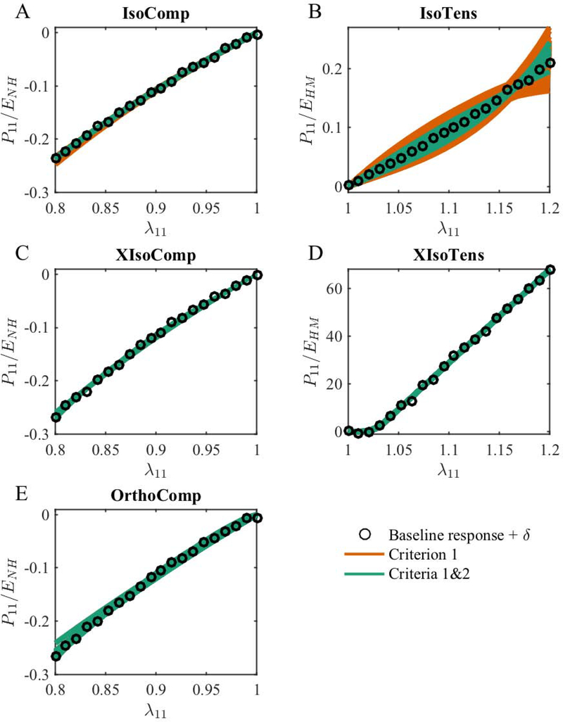
The accepted fits arising from different initial guesses based on only Criterion 1 (orange lines) and Criteria 1&2 (green lines) for the (A) IsoComp, (B) IsoTens, (C) XIsoComp, (D) XIsoTens, and (E) OrthoComp models. All the model fits closely matched their corresponding baseline (“experimental”) stress response, and in most cases, the fits essentially fully overlapped. Note that in each case, the virtually overlapping fits correspond to different sets of parameters arising from different initial guesses. The plotted quantity is the axial component of the Piola-Kirchhoff stress normalized by the baseline parameter value of the matrix modulus. The symbols show the baseline stress with added noise (δ).

In order to calculate the stress-stretch response (for both the baseline response and during optimization), we discretized λ₁ range into 20 steps over the specified ranges, and for each step we incremented (for tension) or decremented (for compression) λ₁ starting at λ₁ = 1. At each value of λ₁, a nonlinear least squares optimization method was used to calculate values of ${\tilde{\lambda }}_2$ and ${\tilde{\lambda }}_3$ that force the “22” and “33” components of the trial stress tensor $\tilde{\mathbf{P}}$ to zero by requiring

$$f({\tilde{\lambda }}_2,{\tilde{\lambda }}_3;{\lambda }_1)=\zeta ({\tilde{P}}_{22}^2+{\tilde{P}}_{33}^2)=0$$ 3)

where ζ was a penalty factor (ζ = 10⁶) which was chosen based on our pilot studies to improve of the optimization and had no effect on the final values of λ₂ and λ₃. Note that this use of optimization to calculate λ₂ and λ₃ is separate from the parameter optimization. Finally, we used the standard continuum mechanics formula (P = ∂Ψ/∂F) to calculate the Piola-Kirchhoff stress from the Helmholtz free energy expressions (Appendix A).

2.4. Baseline parameter values

Representative material parameters from sclera in compression and tendon in tension were used to create the baseline “experimental” tissue stress-stretch data for each constitutive model (Table 1). Specifically, the baseline parameter values were chosen to represent peripapillary sclera for the compression models (IsoComp, XIsoComp, and OrthoComp), and tendon for the tension models (IsoTens, and XIsoTens). The only dimensional parameters in the constitutive relations were the Young moduli (E_NH, E_HM, and E_f). We nondimensionalized the models’ stress-stretch responses by normalizing the stress by the baseline parameter’s matrix modulus value in each model (i.e., axial stress is reported as P₁₁/E_NH for the compression models and P₁₁/E_HM for the tension models). Further, we set the ratio of E_f/E_NH to be 100 for the XIsoComp and OrthoComp models, and set E_f/E_HM to be 200 for the XIsoTens model, according to experimental data on sclera [28] and tendon [29].

2.5. Multi-start optimization

Parameters were identified by multi-start nonlinear least-squares optimization (NLSQ) with a Monte-Carlo-type approach. We first numerically implemented the five constitutive models (IsoTens, IsoComp, XIsoTens, XIsoComp, OrthComp) in MATLAB, which takes axial deformation and constitutive model parameters as input, imposes the boundary conditions, and returns the Piola stress and deformation gradient tensors as the outputs. Using a fixed set of parameters for each model we calculated the mechanical response and designated this as the baseline response. We then separately performed a multi-start NLSQ optimization routine for each model in an attempt to duplicate this baseline stress response.

To fit the “experimental” axial stress (AS)-axial stretch data, we minimized an objective function, f_AS, defined as

$$f_{AS}\left(P_{11};\mathit{p}\right)=\sqrt{\frac{{\sum }_{i=1}^n{\left(P_{11,i}-\left({\overline{P}}_{11,i}+{\delta }_i\right)\right)}^2}{n}}$$ (4)

where P₁₁ is the axial component of the computed stress, ${\overline{P}}_{11,i}$ is the corresponding component of the baseline (“experimental”) stress, p is the set of model parameters, n =20 is the number of discretization steps over the range of λ₁, and i is an index identifying the discretization step. In the above, δ_i is a Gaussian noise term (std(δ) = 1% of the maximum stress) added to the calculated baseline stress response to mimic experimental noise (e.g., device error). This noise level was chosen based on the expected noise from a commercial load cell, which is commonly 0.25% of the nominal rating of the load cell (see for example [30]) and the assumption that the load cell is operating at 50% of the nominal rating, plus added noise due to other sources (e.g., displacement accuracy and fixture compliance).

The multi-start optimization procedure used the interior-point algorithm (fmincon, MATLAB[31]) with a wide search space (Table 1) and 600 random initial guesses (grid size) per parameter. The stopping limit for the algorithm’s objective function was 10⁻⁶ of the normalized baseline matrix modulus. The initial guesses were generated using Latin hypercube sampling, which divides the sampling range into equal regions according to the grid size and generates a random sampling of the search space (lhsdesign, MATLAB). Our pilot studies indicated that this sampling method avoided clustering (nucleation) of random numbers in the sampled values that can potentially bias the optimization outcomes.

Any fit with an objective function value of less than 10 times the added noise was accepted as a solution (Criterion 1):

$$f_{AS}\le 10\mathrm{std}\left({\delta }_i\right)$$ (5)

This quantitative criterion was chosen because it provides a consistent basis across the different models for assessing the quality of the fit, and because its upper limit (f_AS = 10 std(δ_i)) produces a reasonable fit quality (see supplementary Figure S1).

2.6. Including information about lateral strain (LS) predictions

It was immediately evident that the baseline stress-stretch response could be accurately reproduced by many parameter values (see Results), and thus we added a second assessment criterion. We chose this criterion based on the quality of the lateral strain (LS) prediction because we observed that lateral strain predictions were variable across the accepted set of stress-stretch fits. We defined a second objective function, f_LS, as

$$f_{LS}\left(e_{22};\mathit{p}\right)=\sqrt{\frac{{\sum }_{i=1}^n{\left(e_{22,i}-{\overline{e}}_{22,i}\right)}^2}{n}}$$ (6)

where e₂₂ is the “22” component of the Lagrangian strain, and other notation is as in equation (4). Similar to the stress fitting criterion, we defined a second criterion for accepting a fit (Criterion 2):

$$f_{LS}\le 0.1\max \left(e_{22}\right)$$ (7)

We applied Criterion 2 to the fits that met Criterion 1 (Figure 1), and refer to both criteria together as Criteria 1&2. Note that f_LS was not used to drive parameter optimization; instead it was used to compare the solutions obtained by parameter optimization based on f_AS.

Note that the “22” and “33” components of the lateral strain were identical (e₂₂ = e₃₃) for most of the models, evaluation of f_LS(e₂₂; p) implies evaluation of f_LS(e₃₃; p). The exception was the OrthoComp model, since the anisotropy of the continuous fiber distribution caused the in-plane deformation to differ along the 2 and 3 axes. Therefore, for this case, we defined a slightly modified objective function for Criterion 2

$$f_{LS,OC}=\frac{1}{2}\left[f_{LS}\left(e_{22};\mathit{p}\right)+f_{LS}\left(e_{33};\mathit{p}\right)\right]\le 0.1\frac{1}{2}\left[\max \left(e_{22}\right)+\max \left(e_{33}\right)\right].$$ (8)

2.7. Assessment of identifiability criterion

The identifiability of each material parameter for each constitutive model was assessed by comparing the optimized parameter values to the baseline parameter values. We defined γ to quantify the identifiability of each constitutive model parameter as

$$\gamma =\left|\frac{\mathrm{median}\left(p_{fit}\right)-p_0}{p_0}\right|$$ 9)

where p_fit is the fitted (optimized) parameter value and p₀ is its corresponding baseline parameter value. A parameter was said to be identifiable if the corresponding γ was less than 5%. This threshold was chosen because a 5% deviation is commonly taken as an acceptable error in engineering applications; however, this threshold could be adjusted according to the application (see discussion below).

3. Results

3.1. Stress fitting results

All the acceptable fitted responses obtained by the optimization of the axial stress (Criterion 1; Eq. 5) closely matched the baseline (“experimental”) stress response (Figure 2). The number of acceptable solutions found through optimization for the IsoComp model was 600/600, i.e., all 600 random initial guesses resulted in fits that satisfied Criterion 1. The corresponding statistics for the IsoTens, XIsoComp, XIsoTens, and OrthoComp models were 252/600, 482/600, 577/600, and 481/600, respectively. However, these fitted responses resulted in non-unique parameter values, i.e., there were many solutions that acceptably reproduced the baseline uniaxial stress-stretch response.

3.2. Lateral strain predictions

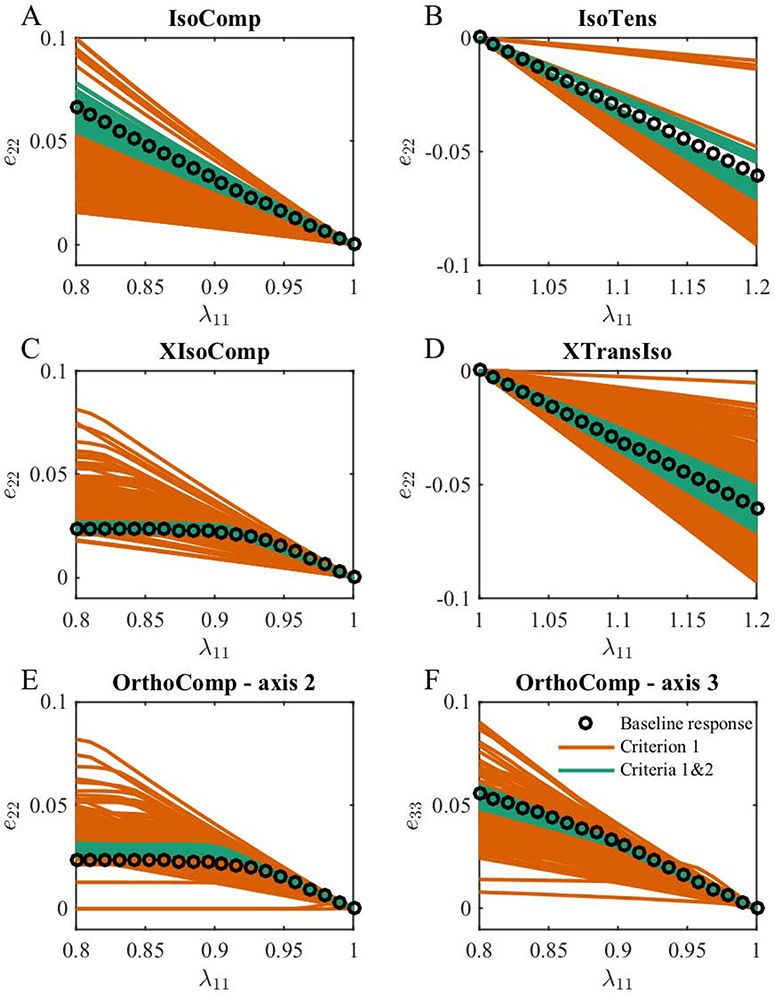
To investigate the possibility of improving identifiability, we used the lateral strain prediction as a second criterion after optimizing to the axial stress response (Criteria 1&2). Solutions meeting both criteria closely matched both the baseline axial stress-stretch response (Criteria 1&2; Figure 2) and lateral strain response (Criteria 1&2; Figure 3), with multiple acceptable fits overlapping each other and the baseline response (Figures 2 and 3). Importantly, by using both Criteria 1&2, the nonlinear baseline response in XIsoComp (Figure 3C) and the anisotropy in OrthoComp lateral strains (the difference between e₂₂ and e₃₃) were captured.

Figure 3:

The lateral strain predictions vs. axial stretch based on Criterion 1 (red) and Criteria 1&2 (green) for (A) IsoComp, (B) IsoTens, (C) XIsoComp, (D) XIsoTens, and (E, F) OrthoComp models. We show two plots for the OrthoComp model due to different lateral strain magnitudes in this orthotropic model, i.e. e₂₂ ≠ e₃₃. It is evident that using only Criterion 1 yields lateral strain predictions that do not coincide with the baseline (“experimental”) lateral strain, while using Criteria 1&2 significantly improves the match between the fitted results and the baseline values.

The numbers of solutions that met both Criteria 1 and 2 were smaller than the ones identified by only Criterion 1. For example, for the IsoComp model, 600/600 fits were acceptable when using only Criterion 1, while using both Criteria 1&2 reduced this to 56/600. For the IsoTens, XIsoComp, XIsoTens and OrthoComp models, the number of successful fits was 35/600, 19/600, 110/600, and 27/600 solutions, respectively.

3.3. Identifiability of parameters

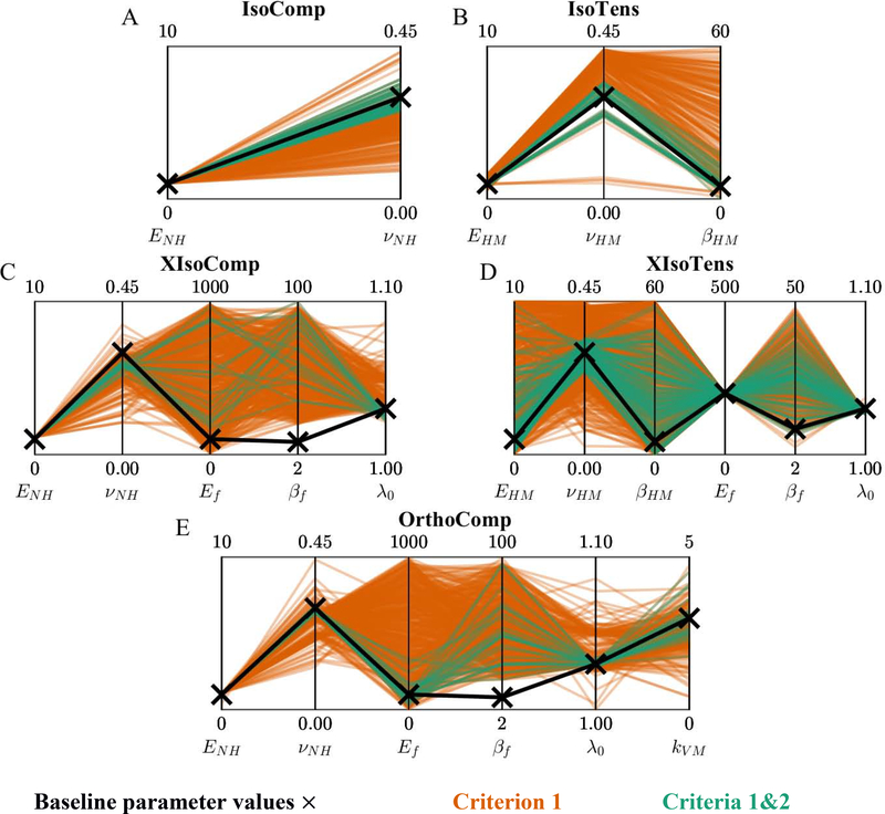
Because multiple solutions were generated with different sets of parameters that matched the axial stress and lateral strain (Figures 2 and 3), we assessed the identifiability of the material parameters by comparing the fitted parameter values to the baseline parameter values. It is convenient to present these comparisons using parallel coordinates plots [19], [32], in which each fitted parameter can be compared directly to its baseline parameter value in a single plot (Figure 4). Histograms describing the distribution of fitted parameter values are available in the supplementary figures (Figure S2–4). In addition, we quantified identifiability through the quantity γ (Table 2), reflecting the material parameter’s error with respect to the baseline parameter value (Eq. 9).

Figure 4:

Parallel coordinate representation of the fitted parameter values for the (A) IsoComp, (B) IsoTens, (C) XIsoComp, (D) XIsoTens, and (E, F) OrthoComp models. Fits are shows based on only Criterion 1 (red) and Criteria 1&2 (green). In each plot the vertical lines represent a single model parameter, enabling depiction the high-dimensional model parameters in a single graph.

Table 2:

Results of identifiability analysis. A γ value ≤ 0.05 indicates that the parameter was successfully identified, where a larger value indicates lack of identification.

Model	Criteria	$\mathbf{Identifiability}\mathbf{parameter}\mathbf{\gamma }\text{:=}\left|\frac{\mathbf{median}({\mathit{p}}_{\mathit{fit})}-{\mathit{p}}_{\mathbf{0}}}{{\mathit{p}}_{\mathbf{0}}}\right|$							# of parameters identified
		Matrix			Fibers
		ENH	νNH
IsoComp	1	0.013 *	0.249						1/2
	1&2	0.001 *	0.046 *						2/2
		EHM	νHM	βHM
IsoTens	1	0.015 *	0.364	4.924					1/3
	1&2	0.029 *	0.035 *	0.250					2/3
		ENH	νNH		Ef	βf	λ0
XIsoComp	1	0.055	0.114		4.115	4.998	0.003 *		1/5
	1&2	0.034 *	0.127		4.036	6.105	0.004 *		2/5
		EHM	νHM	βHM	Ef	βf	λ0
XIsoTens	1	3.200	0.229	4.656	0.015 *	1.617	0.003 *		2/6
	1&2	0.684	0.009 *	3.333	0.012 *	1.606	0.003 *		3/6
		ENH	νNH		Ef	βf	λ0	kVM
OrthoComp	1	0.023 *	0.081		4.110	4.360	0.001 *	0.158	2/6
	1&2	0.021 *	0.007 *		0.128	3.967	0.00003 *	0.032 *	4/6

^*γ ≤ 0.05

3.3.1. Isotropic models (IsoComp and IsoTens)

For the IsoComp model, when only considering the stress fits (Criterion 1), the matrix modulus (E_NH) was consistently identified (γ < 0.05), yet the matrix Poisson’s ratio (ν_NH) was not (Table 2 and Figure 4A). When considering both stress fits and lateral strain predictions (Criteria 1&2) the deviation from baseline parameter values decreased and both parameters were consistently identified (γ < 0.05; Table 2 and Figure 4A).

For the IsoTens model, the modulus E_HM was the only parameter that could be identified when solely matching the stress response (Criterion 1), and this parameter had the smallest deviation from its baseline parameter value among the parameters of the IsoTens model (γ < 0.05; Table 2 and Figure 4B). Interestingly, the Poisson’s ratio (ν_HM) and nonlinearity parameter (β_HM) took almost any value in the search range, with the ν_HM distribution being skewed toward 0.5 and no meaningful concentration of values for β_HM (Figure 4B). When applying Criteria 1&2, identifiability improved for all parameters; however, β_HM could still not be identified (Table 2 and Figure 4B). The lack of identifiability in the nonlinearity parameter was a common behavior observed in many of the other models (see below).

3.3.2. Transversely isotropic models (XIsoComp and XIsoTens)

As expected, due to there being more parameters in the transversely isotropic models, the distribution of parameter values was larger and more complex than for the isotropic cases. In the XIsoComp model, only the fiber uncrimping stretch λ₀ was identified when Criterion 1 was used (Table 2 and Figure 4C). The matrix modulus, E_NH, had a γ value 0.055, and despite it having a narrow distribution, it just failed to be classed as identifiable based on our identifiability threshold of γ < 0.05. Identifiability was improved by applying both Criteria 1&2, which maintained the identifiability of λ₀ and caused E_NH to become identifiable (Table 2 and Figure 4C). However, values of the fiber modulus (E_f) and nonlinearity parameter (β_f) were essentially randomly distributed in the search space, and the model was not sensitive to changes in them (Figure 4C).

For the XIsoTens model, none of the matrix parameters were identifiable when considering only Criterion 1 (Table 2 and Figure 4D). However, the fiber parameters, namely fiber modulus (E_f) and uncrimping stretch (λ₀), were identifiable and had a narrow distribution (γ < 0.05; Table 2 and Figure 4D). Again, the fiber nonlinearity parameter (β_f) was not identifiable and had a median value of approximately twice its baseline parameter value (Table 2). When enforcing both Criteria 1&2, the identifiability of the matrix parameters was improved (Figure 4D); however, only ν_HM was identified (γ < 0.05; Table 2). The fiber parameters remained identifiable, and the addition of Criteria 1&2 had almost no effect on their values (Table 2 and Figure 4D).

3.3.3. Orthotropic model (OrthoComp)

When considering only Criterion 1, E_NH was the only matrix parameter that was identified and the uncrimping stretch λ₀ was the only fiber parameter that was identified (Table 2 and Figure 4E). Similar to XIsoComp, the identifiability of fiber parameters was poor, with the fiber modulus E_f and the fiber nonlinearity parameter β_f not identifiable and having nearly uniform distributions over the search range (Figure 4E). The von Mises factor for the fiber distribution (k_VM) was centered around 2.5 but did not meet the criterion for identifiability (Table 2 and Figure 4E). Applying Criteria 1&2 improved the identifiability of E_NH and λ₀ as compared to Criterion 1 alone (decreased γ), and caused two additional parameters (ν_NH and k_VM) to become identifiable (Table 2 and Figure 4E). However, fiber parameters E_f and β_f remained unidentifiable, similar to the XIsoComp case.

3.4. Identification of Poisson’s ratio

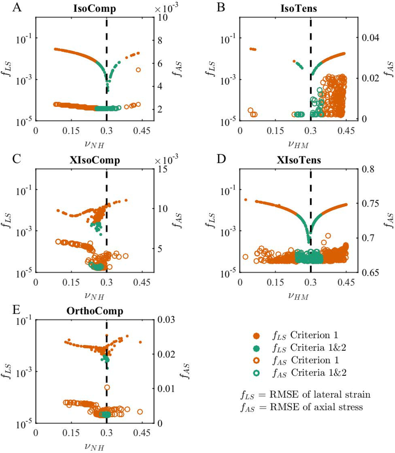
The Poisson’s ratio of the matrix was able to be identified when using Criteria 1&2 for all the models except for XIsoComp (Table 2). Because Poisson’s ratio can be experimentally measured from lateral strain, it was of interest to further investigate the identification of Poisson’s ratio. We visualized the relationship between the value of the optimized (fitted) matrix Poisson’s ratio and the values of the objective functions f_AS and f_LS, for axial stress and lateral strain, respectively. In general, while f_LS changed by almost two orders of magnitude due to a change in Poisson’s ratio, f_AS was not particularly sensitive to Poisson’s ratio (Figure 5). In compression, f_AS showed some dependence on Poisson’s ratio for the IsoComp, XIsoComp, and the OrthoComp models (Figure 5A, 5C, 5E). However, in tension f_AS was completely insensitive to Poisson’s ratio for the IsoTens and XIsoTens models. In contrast, the curves of f_LS versus ν_NH or ν_HM showed sharp minima at the respective baseline values (Figure 5A–E) in both compression and tension. We note that the minimum of the f_LS vs. Poisson ratio plot was less pronounced for the XIsoComp and the OrthoComp models (Figure 5C and E).

Figure 5:

The relation between the objective function values and matrix Poisson’s ratios. We show objective function values for both lateral strain (solid circles; f_LS; left axis log-scale) and axial stress (open circles; f_AS; right axis linear-scale) for the (A) IsoComp, (B) IsoTens, (C) XIsoComp, (D) XIsoTens, and (E) OrthoComp models. In each model, the fits that met Criteria 1&2 had lower f_LS values compared to fits that only met Criterion 1, which occurred near the baseline Poisson’s ratio for each model (dashed vertical line). However, this trend was not consistent when considering f_AS, where only the IsoComp and XIsoComp models (A and C) showed improved fitting with Criteria 1&2. This indicates that although lateral deformation prediction is sensitive to Poisson’s ratio, the same axial stress fits could be achieved with different Poisson’s ratios.

4. Discussion

We here investigated the identifiability of constitutive relationship parameters from uniaxial tension and compression mechanical testing of several types of materials: isotropic, transversely isotropic, and orthotropic. These material symmetries and the associated uniaxial testing are relevant to a wide range of applications in fibrous soft tissues, biomaterials, and tissue-engineered constructs. We used baseline material properties relevant for the sclera in compression and for tendon in tension and assessed model parameter identifiability based on a numerical metric (Eq. 9). This generalized approach is outlined in Supplemental Table S1 for other applications.

Our results showed that, when only the axial stress-stretch response was used in curve-fitting, none of the constitutive models were fully identifiable, i.e., the same stress-stretch response could be generated by different sets of parameter values. We further showed that the identifiability of parameters was greatly improved if information about lateral strain was included in the parameter identification.

4.1. Identifiability of parameters in isotropic models using uniaxial testing

We considered two isotropic material models; although isotropy is atypical in physiological tissue, isotropic biomaterials, such as hydrogels, are widely used [33]. Our results indicated that even the parameters of the simplest nonlinear constitutive relations were not fully identifiable from a uniaxial test (Figure 4A and B). These results are consistent with studies on the identifiability of parameters in isotropic elastic materials [11], [14], [34]. However, note that the modulus was identified from the stress-stretch response in both isotropic models. Since only a measure of stiffness is sought in many studies, a uniaxial test could be sufficient for that purpose; however, other material parameters (ν and β) were not identifiable and are not reliable when determined by uniaxial testing. Since all these material parameters are needed for finite element analysis, fitting to only stress-stretch data is likely to be insufficient for subsequent use in finite element analysis.

4.2. Effect of aligned fiber reinforcement in tensile loading

In the transversely isotropic models in our study, the fiber properties were mostly identifiable, but the matrix parameters could not be identified from only the stress-stretch response. This was particularly noticeable in the transversely isotropic tension (XIsoTens) model (representing tendon, Figure 2D, Figure 4D, and Table 2). Even with the addition of lateral strain (Criterion 2), it was not possible to identify matrix modulus (Table 2). This is likely due to the large difference between the stiffness of fibers and matrix in tendon [35]. Other modes of loading such as lateral compression or osmotic loading have been used to remedy this problem [18], [29], [36]; however, it is likely that in those modes of loading (such as lateral compression), the identifiability of other parameters would be lost (e.g., fiber modulus). A careful a priori identifiability check is needed to design the loading mode and analyze the experimental results before relying on optimized material parameters.

4.3. Effect of fiber distribution in compression loading

A distribution of fibers perpendicular to the compressive loading direction occurs in several tissues, including the sclera of the eye. When the samples are small, such as in rodent sclera, inverse finite element modeling can be used to determine material parameters, including the spatial distribution of fiber concentration factor, k_VM [4]. Our results showed that, for such anisotropic models in compression (XIsoComp and OrthoComp), the identifiability of parameters is poor (Figure 4 and Table 2), particularly for the fiber modulus and nonlinearity. Surprisingly, the identifiability of the parameters in the orthotropic model (OrthoComp) was superior to that in its transversely isotropic counterpart (XIsoComp). This indicates that anisotropy can improve the identifiability of model parameters and highlights the complex interplay between tissue anisotropy and material parameter identifiability.

4.4. Improving identifiability of model parameters

It is expected that the addition of more experimental information in data fitting would improve the identifiability of parameters. Assessment of the number of identified parameters in each model allowed us to make comparisons between the cases that only used axial stress fits and the ones that also included the lateral strain predictions, which indicated an improvement in the identifiability of the parameters. There are several approaches to include additional experimental data in the fitting. For example, experimental measurement of parameters related to fiber orientation and distribution [27], [37] and fiber uncrimping [38], [39], micromechanical modeling [15], and multi-axial mechanical testing [34], [40], are potential approaches to improve parameter identifiability. In micromechanical models, for example, the parameters that influence the mechanical response are assumed, while our method provides empirical evidence for how those parameters can be determined. Therefore, this method can be used as an adjunct to micromechanical modeling.

In this study, we demonstrated that the inclusion of a criterion based on lateral strain when selecting acceptable fits improved parameter identifiability in all the models. However, the most effective approach is not clear and is likely problem-dependent. Examples of other methods include fitting an analytical expression for Poisson’s ratio to experimental lateral deformation [41], or using the direct measurement of Poisson’s ratio, which is appropriate for linear elastic materials and small deformations [11]. However, due to tissue nonlinearity, these methods are not always feasible. The most generalizable options are to either conduct a multi-objective optimization by fitting experimental stress and lateral strain responses (e.g., measured using digital image correlation [42]) simultaneously [43], or to assess the predictions of lateral strain following optimization on the axial stress-stretch response, as was done in this study. We should add that an identifiability analysis is most effective if done prior to experimental data collection. By doing so, such an analysis will provide a means to assess the match between the constitutive model and the intended experimental measurement, and suggest appropriate experimental designs to measure the material parameters using the proposed constitutive model [44].

4.5. Sensitivity of fit results to Poisson’s ratio

Our analysis of the relationships among matrix Poisson’s ratio and the values of the objective functions for axial stress fit (f_AS) and lateral strain (f_LS) revealed that, although the stress fit could be practically insensitive to a change in Poisson’s ratio, the lateral strain, as expected, was highly sensitive to Poisson’s ratio and f_LS showed a clear minimum near the baseline parameter value for each model (Figure 5). This indicates that, although several values for Poisson’s ratio can result in an acceptable stress-stretch response, only the fits with the matrix Poisson’s ratio closest to the baseline parameter value produce a good lateral strain prediction. Further, the lack of dependence of f_AS on Poisson’s ratio indicates that even by using another optimization algorithm that seeks a possible global minimum, the problem of identifiability would persist. In other words, non-identifiability means that no algorithm will retrieve the parameter. In these cases that multiple local attractors (multiple local minima) exist, clustering analysis (e.g., using principal component analysis) and direct inspection of the cost-function residuals can be useful. These findings are also consistent with prior studies using separate orthotropic constitutive relations showing a lack of sensitivity of axial stress to a change in transverse Poisson’s ratio [45] and indicating the importance of considering the lateral deformations in identifying the mechanical material properties of anisotropic materials [42], [45].

It is worth noting that the identifiability analysis presented here is different than, but complementary to, sensitivity analysis. Sensitivity analysis determines the effect of uncertainty and variation in the input parameters on the model predictions [12], [40], [46]. Although the multi-start optimization method that we used for identifiability analysis shares some aspects with sensitivity analysis, their objectives are different. In multi-start optimization, the objective is to find the parameter sets that produce similar experimental observations, while in a sensitivity analysis, the objective is to study the effect of uncertainty of an input parameter on the outputs. Therefore, although beyond the scope of this study, a sensitivity analysis can be used in concert with an identifiability analysis to understand the effect of variation of each material parameter value in the simulated model responses.

4.6. Limitations

This study has some limitations. First, although multi-start optimization eliminated dependence of the curve-fitting results on the initial guess, a user-dependent range of parameters is still needed, which could potentially impact the results. However, selecting a wide search space, dense sampling of this space should, and using sub-space optimization, where some of the parameters are kept fixed, could minimize this effect and are possible strategies to better study identifiability of material parameters. Second, we assumed a relatively small noise amplitude in the baseline (“experimental”) stress response. Although this was reasonable for macroscale and tissue testing, in some micro- and meso-scale tests, larger noise levels might be expected, which would affect uncertainty and identifiability. Third, we selected criteria and thresholds for acceptable fits (objective functions f_AS and f_LS based on root-mean squared errors) and for identifiability (γ < 5%) which were reasonable for our application. Nonetheless, the threshold, criteria, and the normalization formula to calculate γ are selected by the user, and other values and normalization methods could be chosen. Alternative identifiability criteria such as the rank deficiency of the Fisher information matrix in Bayesian analysis, which can also take into consideration parameter distributions, are also prone to similar subjective choices of a threshold, where there is a need for the definition of a threshold of a “zero eigenvalue” [12]; however, the multi-start optimization framework of this paper is simple to implement. Thus, it is highly practical and does not need any special advanced statistical methods such as used in Bayesian analysis, and in fact results in similar outcomes [12]. There are many other examples of identifiability criteria in different disciplines [9], [10], which are mostly application-driven. Selecting the best identifiability criteria and threshold is problem-dependent and should be adjusted depending on the application. For example, our analysis used the standard root mean square of errors as the cost function (Eq. 4); however, using different forms of the cost function, such as sub-space optimization, will change the identifiability of material parameters. If such alternative forms are used, identifiability should be checked separately using the approach described in this study [47], [48].

4.7. Summary and conclusions

We investigated the identifiability of material parameters for fiber-reinforced tissues by using nonlinear constitutive modeling and multi-start optimization. Our results indicated that multiple sets of parameters can produce the same stress-stretch responses and that, therefore, axial stress response alone is likely to be insufficient to identify tissue material properties. The addition of a selection criterion based on lateral strain significantly improved parameter identifiability; however, even then, some parameters remained unidentifiable. This study is novel in that it provides a systematic and generalizable approach to assess the identifiability of material parameters in a straightforward framework, and the approach is translatable to many studies of parameter identification. Due to the simplicity of implementing multi-start optimization, it could easily be extended to study viscoelasticity and other inelastic behaviors and other experimental conditions (e.g., different loading modes). In conclusion, we recommend conducting an identifiability analysis as a necessary step for any material parameter data-fitting study and suggest multi-start optimization as an effective tool for conducting curve fitting to evaluate the mechanical parameters of tissue.

Statement of Significance.

Data fitting is a powerful technique commonly used to extract tissue material parameters from experimental data, and which thus has applications in tissue biomechanics and engineering. However, the problem of “uniqueness” or “identifiability” of the fit parameters is a significant issue, limiting the fit results’ validity. Here we provide a systematic method to evaluate data fitting and assess the uniqueness of results in the tissue constitutive models. Our study confirmed that the uniaxial stress-stretch experimental data are not adequate to identify all the tissue material parameters and provides a robust approach to check for parameter identifiability in other studies. This study is of potential interest to a wide range of readers because of its application for the characterization of other engineering materials while addressing the problem of uniqueness of the fitted results.

Appendix A: Constitutive relations

Isotropic models

For the isotropic model in compression (IsoComp) we used a compressible neo-Hookean material description with Helmholtz free energy defined as [24]

$${\mathrm{\Psi }}_{NH}\left(I_1,J\right)=\frac{{\mu }_{NH}}{2}\left(I_1-3\right)-{\mu }_{NH}\ln J+\frac{{\lambda }_{NH}}{2}{(\ln J)}^2$$ (1A)

where “NH” stands for neo-Hookean, I₁ is the first invariant of the right Cauchy-Green strain tensor (C = F^T · F; F is the deformation gradient tensor) and J (the Jacobian of the deformation) is the square root of the third invariant of C. The invariants are of C are defined in the standard manner as

$$I_1=\mathrm{tr}(\mathbf{C}),I_2=\frac{1}{2}\left(\mathrm{tr}{(\mathbf{C})}^2-\mathrm{tr}\left({\mathbf{C}}^2\right)\right),\text{and}{I}_3^{1/2}=J=\det {(\mathbf{C})}^{\frac{1}{2}}.$$ (2A)

Further, in Eq. 1A ${\lambda }_{NH}=E_{NH}{v}_{NH}/\left[\left(1+v_{NH}\right)\left(1-2v_{NH}\right)\right]$, and ${\mu }_{NH}=E_{NH}/\left[2\left(1-v_{NH}\right)\right]$ are the Lamé parameters of the matrix, E_NH is the Young’s modulus, and ν_NH is Poisson’s ratio. The neo-Hookean constitutive relation has two independent material parameters (E_NH and ν_NH; Table 1).

For the isotropic model in tension (IsoTens) we used a Holmes-Mow material description with Helmholtz free energy defined as [25]

$${\mathrm{\Psi }}_{HM}\left(I_1,I_2,J\right)=C_0\left(\exp \left[Q\left(I_1,I_2,J\right)\right]-1\right)$$ (3A)

where “HM” stands for Holmes-Mow, and C₀ and Q are given by

$$C_0=\frac{{\lambda }_{HM}+2{\mu }_{HM}}{4{\beta }_{HM}}$$ (4A.a)

$$Q={\beta }_{HM}\frac{2{\mu }_{HM}-{\lambda }_{HM}}{{\lambda }_{HM}+2{\mu }_{HM}}\left(I_1-3\right)+\frac{{\beta }_{HM}{\lambda }_{HM}}{{\lambda }_{HM}+2{\mu }_{HM}}\left(I_2-3\right)+\ln J^2$$ (4A.b)

Here, λ_HM and μ_HM are the standard Lamé parameters, β_HM is the nonlinearity parameter (β_HM > 0), and I₁ and I₂ are the first and second invariants of the right Cauchy-Green deformation tensor. For convenience, we show results in terms of Young’s modulus, E_HM, and Poisson’s ratio, ν_HM instead of the Lamé parameters, which are related to E_HM and ν_HM by the following relations: ${\lambda }_{HM}=E_{HM}{v}_{HM}/\left[\left(1+v_{HM}\right)\left(1-2v_{HM}\right)\right]$, and ${\mu }_{HM}=E_{HM}/\left[2\left(1-v_{HM}\right)\right]$. This constitutive model has three independent material parameters: E_HM, ν_HM, and β_HM (Table 1).

Transversely isotropic models

For the transversely isotropic model in compression (XIsoComp), we embedded a continuous fiber distribution in a compressible neo-Hookean matrix (Eq. 1A) [23]. The fibers obeyed the following formulation

$${\mathbf{P}}_{f,dist}={\int }_0^{\pi }g(\theta ){\mathbf{P}}_n\left(I_n(\theta )\right)d\theta$$ 5A)

In this relation, P_f,dist is the first Piola-Kirchhoff stress of the in-plane fibers (2–3 plane; Table 1), P_n is the contribution of the fibers oriented with the unit vector n = cos(θ)e₂ + sin(θ)e₃

$${\mathbf{P}}_n\left(I_n\right)=2\mathbf{F}\cdot \frac{\partial {\mathrm{\Psi }}_f}{\partial \mathbf{C}}=2\mathbf{F}\cdot (\frac{\partial {\mathrm{\Psi }}_f}{\partial I_n}\mathit{n}\otimes \mathit{n})$$ 6A)

and g(θ) is the modified von Mises distribution, previously used to describe the fiber distribution in scleral tissue [26], [27]

$$g(\theta )=\frac{1}{\pi I_0\left(k_{VM}\right)}\mathit{exp}[k_{VM}\mathit{cos}\left(2\left(\theta -{\theta }_p\right)\right)]$$ 7A)

In this relation, I₀ is the modified Bessel function of the first kind, k_VM is the fiber concentration factor (k_VM = 0 for an isotropic in-plane distribution), and θ_p is the modal fiber orientation. We set θ_p to zero, so that g_max = g(0). To evaluate this integral numerically we used a left Reimann numerical summation. In the numerical implementation of this integral we used a left Reimann numerical sum. In Eq. 6A, Ψ_f is the Helmholtz free energy of the fiber phase (the subscript ‘f’ stands for fibers), defined as:

$${\mathrm{\Psi }}_f=\{\begin{array}{ll}0\hfill & I_n<1\hfill \\ \frac{\xi }{2{\beta }_f}{\left(I_n-1\right)}^{{\beta }_f}\hfill & 1\le I_n\le I_0\hfill \\ E_f\left(I_0^{\frac{1}{2}}-I_n^{\frac{1}{2}}\right)+B\left(I_n-I_0\right)+{\mathrm{\Psi }}_0\hfill & I_0<I_n\hfill \end{array}$$ (8A)

where I_n is the pseudo-invariant of deformation along a fiber direction defined by unit vector n, i.e.,

$$I_{\mathit{n}}=n\cdot \mathbf{C}\cdot \mathit{n}$$ 9A)

where $\xi =\frac{E_f}{2\left({\beta }_f-1\right)}{\left(I_0-1\right)}^{2-{\beta }_f}$, $B=\frac{E_f}{2}(\frac{I_0-1}{2(\beta -1)}+I_0)$, and ${\mathrm{\Psi }}_0=\frac{\xi }{2\beta }{\left(I_0-1\right)}^{{\beta }_f}$, and it is assumed that fibers do not have a compressive stiffness. Note that this constitutive relation describes the well-known toe-linear response in tendon [20], [21] and this particular form was selected based on its usefulness for 3D finite element simulations [22] (see Section 5.3.7 of the FEBio theory manual v2.9, febio.org). The independent parameters in this constitutive relation for fibers are the tensile fiber modulus, E_f, the fiber nonlinearity parameter, β_f (β_f ≥ 2), and the square of the uncrimping stretch of fibers, I₀ = (λ₀)². In summary, there are five independent material parameters in the XIsoComp model (Table 1): [E_NH, ν_NH] for the matrix and [E_f, β_f, λ₀] for the in-plane fibers, since k_VM is set to zero for the XIsoComp model.

For the transversely isotropic model in tension (XIsoTens), we embedded fibers with a toe-linear response (Eq. 8A) in a Holmes-Mow material (Eq. 3A). The fibers were specified to be parallel to the axial direction (n = e₁). As a result, there are six independent material parameters in the XIsoTens model: [E_HM, ν_HM, β_HM] for the matrix and [E_f, β_f, λ₀] for the fibers (Table 1).

Orthotropic model

For the orthotropic model in compression (OrthoComp) we used the same formulation as in (Eq. 5A–9A), except that the fiber distribution was not assumed to be uniform; that is, k_VM > 0. This resulted in an aligned in-plane fiber distribution, and therefore orthotropic symmetry in the material configuration. This senario is a characteristic of prepapillary sclera [26], [27]. The OrthoComp model has one more material parameter than the XIsoComp model (six independent parameters): [E_NH, ν_NH] for the matrix and [E_f, β_f, λ₀, k_VM] for the fibers.

References

- [1].Donoso-Bravo A, Mailier J, Ruiz-Filippi G, and Vande Wouwer A, “Identification in an anaerobic batch system: global sensitivity analysis, multi-start strategy and optimization criterion selection.,” Bioprocess Biosyst. Eng, vol. 36, no. 1, pp. 35–43, January. 2013, doi: 10.1007/s00449-012-0758-5. [DOI] [PubMed] [Google Scholar]
- [2].Avril S and Evans S, Material Parameter Identification and Inverse Problems in Soft Tissue Biomechanics. 2017. [DOI] [PubMed] [Google Scholar]
- [3].Safa BN, Santare MH, Elliott DM, Lee AH, Santare MH, and Elliott DM, “Evaluating Plastic Deformation and Damage as Potential Mechanisms for Tendon Inelasticity Using a Reactive Modeling Framework,” J. Biomech. Eng, vol. 141, no. 2, p. 101008, July. 2019, doi: 10.1115/1.4041575. [DOI] [PMC free article] [PubMed] [Google Scholar]
- [4].Schwaner SA, Hannon BG, Feola AJ, and Ethier CR, “Biomechanical properties of the rat sclera obtained with inverse finite element modeling,” Biomech. Model. Mechanobiol, May 2020, doi: 10.1007/s10237-020-01333-4. [DOI] [PMC free article] [PubMed] [Google Scholar]
- [5].Sverdlik A and Lanir Y, “Time-dependent mechanical behavior of sheep digital tendons, including the effects of preconditioning.,” J Biomech Eng, vol. 124, no. 1, pp. 78–84, 2002, doi: 10.1115/1.1427699. [DOI] [PubMed] [Google Scholar]
- [6].Kelley CT, Iterative Methods for Optimization. Society for Industrial and Applied Mathematics, 1999. [Google Scholar]
- [7].Vaz M, Cardoso EL, and Stahlschmidt J, “Particle swarm optimization and identification of inelastic material parameters,” Eng. Comput. (Swansea, Wales), vol. 30, no. 7, pp. 936–960, October. 2013, doi: 10.1108/EC-10-2011-0118. [DOI] [Google Scholar]
- [8].Schutte JF, Koh BII, Reinbolt JA, Haftka RT, George AD, and Fregly BJ, “Evaluation of a particle swarm algorithm for biomechanical optimization,” J. Biomech. Eng, vol. 127, no. 3, pp. 465–474, June. 2005, doi: 10.1115/1.1894388. [DOI] [PMC free article] [PubMed] [Google Scholar]
- [9].Kalman RE, “Identifiability and Modeling in Econometrics,” vol. 4, Elsevier, 1983, pp. 97–136. [Google Scholar]
- [10].(Eric) Walter E and Pronzato L, Identification of parametric models from experimental data. Springer, 1997. [Google Scholar]
- [11].Hartmann S and Gilbert RR, “Identifiability of material parameters in solid mechanics,” Arch. Appl. Mech, vol. 88, no. 1–2, pp. 3–26, February. 2018, doi: 10.1007/s00419-017-1259-4. [DOI] [Google Scholar]
- [12].Akintunde AR, Miller KS, and Schiavazzi DE, “Bayesian inference of constitutive model parameters from uncertain uniaxial experiments on murine tendons,” J. Mech. Behav. Biomed. Mater, vol. 96, pp. 285–300, August. 2019, doi: 10.1016/j.jmbbm.2019.04.037. [DOI] [PMC free article] [PubMed] [Google Scholar]
- [13].Holzapfel GA and Ogden RW, “On planar biaxial tests for anisotropic nonlinearly elastic solids. A continuum mechanical framework,” Math. Mech. Solids, vol. 14, no. 5, pp. 474–489, July. 2009, doi: 10.1177/1081286507084411. [DOI] [Google Scholar]
- [14].Ogden R, Saccomandi G, and Sgura I, “Fitting hyperelastic models to experimental data,” Comput. Mech, vol. 34, no. 6, 2004, doi: 10.1007/s00466-004-0593-yi. [DOI] [Google Scholar]
- [15].Rokoš O, Hoefnagels JPM, Peerlings RHJ, and Geers MGD, “On micromechanical parameter identification with integrated DIC and the role of accuracy in kinematic boundary conditions,” Int. J. Solids Struct, vol. 146, pp. 241–259, August. 2018, doi: 10.1016/j.ijsolstr.2018.04.004. [DOI] [Google Scholar]
- [16].Balaban G, Alnaes MS, Sundnes J, and Rognes ME, “Adjoint multi-start-based estimation of cardiac hyperelastic material parameters using shear data.,” Biomech. Model. Mechanobiol, vol. 15, no. 6, pp. 1509–1521, December. 2016, doi: 10.1007/s10237-016-0780-7. [DOI] [PMC free article] [PubMed] [Google Scholar]
- [17].Posik P, Huyer W, and Pal L, “A comparison of global search algorithms for continuous black box optimization.,” Evol. Comput, vol. 20, no. 4, pp. 509–541, 2012, doi: 10.1162/EVCO_a_00084. [DOI] [PubMed] [Google Scholar]
- [18].Safa BN, Bloom ET, Lee AH, Santare MH, and Elliott DM, “Evaluation of Transverse Poroelastic Mechanics of Tendon using Osmotic Loading and Biphasic Mixture Finite Element Modeling,” J. Biomech, vol. 109, p. 109892, June. 2020, doi: 10.1016/j.jbiomech.2020.109892. [DOI] [PMC free article] [PubMed] [Google Scholar]
- [19].Safa BN, Lee AH, Santare MH, and Elliott DM, “Evaluating Plastic Deformation and Damage as Potential Mechanisms for Tendon Inelasticity Using a Reactive Modeling Framework,” J. Biomech. Eng, vol. 141, no. 10, p. 101008, July. 2019, doi: 10.1115/1.4043520. [DOI] [PMC free article] [PubMed] [Google Scholar]
- [20].Tanaka ML, Weisenbach CA, Carl Miller M, and Kuxhaus L, “A Continuous Method to Compute Model Parameters for Soft Biological Materials,” J. Biomech. Eng, vol. 133, no. 7, p. 074502, July. 2011, doi: 10.1115/1.4004412. [DOI] [PubMed] [Google Scholar]
- [21].Lee AH, Szczesny SE, Santare MH, and Elliott DM, “Investigating mechanisms of tendon damage by measuring multi-scale recovery following tensile loading,” Acta Biomater, vol. 57, pp. 363–372, July. 2017, doi: 10.1016/j.actbio.2017.04.011. [DOI] [PMC free article] [PubMed] [Google Scholar]
- [22].Yang B and O’Connell GD, “Swelling of fiber-reinforced soft tissues is affected by fiber orientation, fiber stiffness, and lamella structure,” J. Mech. Behav. Biomed. Mater, vol. 82, no. April, pp. 320–328, 2018, doi: 10.1016/j.jmbbm.2018.03.039. [DOI] [PubMed] [Google Scholar]
- [23].Ateshian GA, Rajan V, Chahine NO, Canal CE, and Hung CT, “Modeling the Matrix of Articular Cartilage Using a Continuous Fiber Angular Distribution Predicts Many Observed Phenomena,” J. Biomech. Eng, vol. 131, no. 6, p. 061003, June. 2009, doi: 10.1115/1.3118773. [DOI] [PMC free article] [PubMed] [Google Scholar]
- [24].Bonet J and Wood RD, Nonlinear Continuum Mechanics for Finite Element Analisys. Cambridge University Press, 1997. [Google Scholar]
- [25].Holmes MH and Mow VC, “The nonlinear characteristics of soft gels and hydrated connective tissues in ultrafiltration,” J. Biomech, vol. 23, no. 11, pp. 1145–1156, 1990, doi: 10.1016/0021-9290(90)90007-P. [DOI] [PubMed] [Google Scholar]
- [26].Girard MJA, Downs JC, Burgoyne CF, and Suh J-KKF, “Peripapillary and posterior scleral mechanics - Part I: Development of an anisotropic hyperelastic constitutive model,” J. Biomech. Eng, vol. 131, no. 5, 2009, doi: 10.1115/1.3113682. [DOI] [PMC free article] [PubMed] [Google Scholar]
- [27].Gouget CLM, Girard MJ, and Ethier CR, “A constrained von Mises distribution to describe fiber organization in thin soft tissues,” Biomech. Model. Mechanobiol, vol. 11, no. 3–4, pp. 475–482, March. 2012, doi: 10.1007/s10237-011-0326-y. [DOI] [PubMed] [Google Scholar]
- [28].Battaglioli JL and Kamm RD, “Measurements of the compressive properties of scleral tissue,” Investigative Ophthalmology and Visual Science, 1984. https://iovs.arvojournals.org/article.aspx?articleid=2159718 (accessed Jul. 03, 2020). [PubMed] [Google Scholar]
- [29].Lynch HA, Johannessen W, Wu JP, Jawa A, and Elliott DM, “Effect of fiber orientation and strain rate on the nonlinear uniaxial tensile material properties of tendon.,” J. Biomech. Eng, vol. 125, no. 5, pp. 726–731, October. 2003, doi: 10.1115/1.1614819. [DOI] [PubMed] [Google Scholar]
- [30].Instron, “2580 Series Static Load Cells.” pp. 1–2, 2016, Accessed: Jun. 08, 2020. [Online]. Available: www.instron.com.
- [31].MathWorks, “Constrained Nonlinear Optimization Algorithms,” MathWorks Doc, pp. 1–15, 2016, Accessed: Oct. 19, 2020. [Online]. Available: https://de.mathworks.com/help/optim/ug/constrained-nonlinear-optimization-algorithms.html#brnpd5f. [Google Scholar]
- [32].Johansson J and Forsell C, “Evaluation of Parallel Coordinates: Overview, Categorization and Guidelines for Future Research,” IEEE Trans. Vis. Comput. Graph, vol. 22, no. 1, pp. 579–588, January. 2016, doi: 10.1109/TVCG.2015.2466992. [DOI] [PubMed] [Google Scholar]
- [33].Chaudhuri O, “Viscoelastic hydrogels for 3D cell culture,” Biomaterials Science, vol. 5, no. 8. Royal Society of Chemistry, pp. 1480–1490, August. 01, 2017, doi: 10.1039/c7bm00261k. [DOI] [PubMed] [Google Scholar]
- [34].Sacks MS and Sun W, “Multiaxial mechanical behavior of biological materials,” Annual Review of Biomedical Engineering, vol. 5. Annu Rev Biomed Eng, pp. 251–284, 2003, doi: 10.1146/annurev.bioeng.5.011303.120714. [DOI] [PubMed] [Google Scholar]
- [35].Böl M, Ehret AE, Leichsenring K, and Ernst M, “Tissue-scale anisotropy and compressibility of tendon in semi-confined compression tests.,” J. Biomech, vol. 48, no. 6, pp. 1092–8, April. 2015, doi: 10.1016/j.jbiomech.2015.01.024. [DOI] [PubMed] [Google Scholar]
- [36].Samuel Salisbury ST, Paul Buckley C, and Zavatsky AB, “Transverse Compression of Tendons,” J. Biomech. Eng, vol. 138, no. 4, p. 041002, February. 2016, doi: 10.1115/1.4032627. [DOI] [PubMed] [Google Scholar]
- [37].Zarei V, Liu CJ, Claeson AA, Akkin T, and Barocas VH, “Image-based multiscale mechanical modeling shows the importance of structural heterogeneity in the human lumbar facet capsular ligament.,” Biomech. Model. Mechanobiol, vol. 16, no. 4, pp. 1425–1438, August. 2017, doi: 10.1007/s10237-017-0896-4. [DOI] [PMC free article] [PubMed] [Google Scholar]
- [38].Fang F and Lake SP, “Multiscale strain analysis of tendon subjected to shear and compression demonstrates strain attenuation, fiber sliding, and reorganization.,” J. Orthop. Res, vol. 33, no. 11, pp. 1704–1712, November. 2015, doi: 10.1002/jor.22955. [DOI] [PubMed] [Google Scholar]
- [39].Buckley MR, Sarver JJ, Freedman BR, and Soslowsky LJ, “The dynamics of collagen uncrimping and lateral contraction in tendon and the effect of ionic concentration.,” J. Biomech, vol. 46, no. 13, pp. 2242–9, September. 2013, doi: 10.1016/j.jbiomech.2013.06.029. [DOI] [PMC free article] [PubMed] [Google Scholar]
- [40].Szczesny SE, “Biaxial Tensile Testing and Constitutive Modeling of Human Supraspinatus Tendon,” J. Biomech. Eng, vol. 134, no. 2, p. 021004, March. 2012, doi: 10.1115/1.4005852. [DOI] [PMC free article] [PubMed] [Google Scholar]
- [41].Swedberg AM, Reese SP, Maas SA, Ellis BJ, and Weiss JA, “Continuum description of the Poisson’s ratio of ligament and tendon under finite deformation.,” J. Biomech, vol. 47, no. 12, pp. 3201–9, September. 2014, doi: 10.1016/j.jbiomech.2014.05.011. [DOI] [PMC free article] [PubMed] [Google Scholar]
- [42].Skacel P and Bursa J, “Poisson’s ratio of arterial wall - Inconsistency of constitutive models with experimental data,” J. Mech. Behav. Biomed. Mater, vol. 54, pp. 316–327, February. 2016, doi: 10.1016/j.jmbbm.2015.09.029. [DOI] [PubMed] [Google Scholar]
- [43].Deb K, “Multi-Objective Optimization Using Evolutionary Algorithms: An Introduction,” 2011. Accessed: May 26, 2020. [Online]. Available: http://www.iitk.ac.in/kangal/deb.htm.
- [44].Holmes JW, “Model first and ask questions later: Confessions of a reformed experimentalist,” J. Biomech. Eng, vol. 141, no. 7, July. 2019, doi: 10.1115/1.4043432. [DOI] [PMC free article] [PubMed] [Google Scholar]
- [45].Latorre M, Romero X, and Montáns FJ, “The relevance of transverse deformation effects in modeling soft biological tissues,” Int. J. Solids Struct, vol. 99, pp. 57–70, November. 2016, doi: 10.1016/j.ijsolstr.2016.08.006. [DOI] [Google Scholar]
- [46].Veres SP, Gastaldi D, and Contro R, “A constituent-based model for the nonlinear viscoelastic behavior of ligaments.,” J. Biomech. Eng, vol. 128, no. 3, pp. 449–57, June. 2006, doi: 10.1115/1.2187046. [DOI] [PubMed] [Google Scholar]
- [47].Schmid H, Nash MP, Young AA, and Hunter PJ, “Myocardial material parameter estimation - A comparative study for simple shear,” J. Biomech. Eng, vol. 128, no. 5, pp. 742–750, October. 2006, doi: 10.1115/1.2244576. [DOI] [PubMed] [Google Scholar]
- [48].Schmid H, Nash MP, Young AA, Röhrle O, and Hunter PJ, “A computationally efficient optimization kernel for material parameter estimation procedures,” J. Biomech. Eng, vol. 129, no. 2, pp. 279–283, April. 2007, doi: 10.1115/1.2540860. [DOI] [PubMed] [Google Scholar]
Associated Data
This section collects any data citations, data availability statements, or supplementary materials included in this article.