Understanding the Microstructure Formation of Polymer Films by Spontaneous Solution Spreading Coating with a High‐Throughput Engineering Platform

Abstract

An important step of the great achievement of organic solar cells in power conversion efficiency is the development of low‐band gap polymer donors, PBDB−T derivatives, which present interesting aggregation effects dominating the device performance. The aggregation of polymers can be manipulated by a series of variables from a materials design and processing conditions perspective; however, optimization of film quality is a time‐ and energy‐consuming work. Here, we introduce a robot‐based high‐throughput platform (HTP) that is offering automated film preparation and optical spectroscopy thin‐film characterization in combination with an analysis algorithm. PM6 films are prepared by the so‐called spontaneous film spreading (SFS) process, where a polymer solution is coated on a water surface. Automated acquisition of UV/Vis and photoluminescence (PL) spectra and automated extraction of morphological features is coupled to Gaussian Process Regression to exploit available experimental evidence for morphology optimization but also for hypothesis formulation and testing with respect to the underlying physical principles. The integrated spectral modeling workflow yields quantitative microstructure information by distinguishing amorphous from ordered phases and assesses the extension of amorphous versus the ordered domains. This research provides an easy to use methodology to analyze the exciton coherence length in conjugated semiconductors and will allow to optimize exciton splitting in thin film organic semiconductor layers as a function of processing.

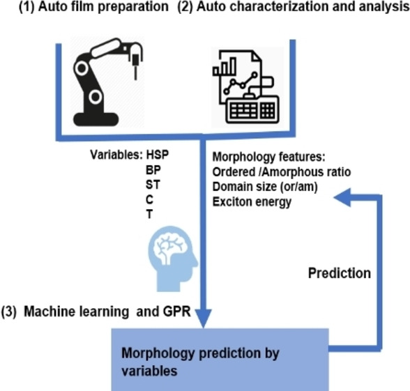
A machinery of information: A high‐throughput platform (HTP) is developed for automated preparation and characterization of polymer films by spontaneous film spreading coating. In combination with Gaussian Process Regression, the microstructure information of polymer films can be successfully predicted, which provides us the possibility to accelerate the decipherment of process−structure−property relationships for functional polymer films.

Introduction

Up to now, solution‐processed organic solar cells (OSCs) have shown a great potential for efficient and environmentally friendly large area production. The power conversion efficiency (PCE) has exceeded 18 % based‐on polymer donors and non‐fullerene acceptors (NFA).[ ¹ , ² ] The class of PBDB−T based polymers, consisting of 2‐alkylthiophene‐substituted benzo[1,2‐b:4,5‐b′]dithiophene (BDT) and 1,3‐bis(thiophen‐2‐yl)‐5,7‐bis(2‐ethylhexyl)benzo‐[1,2‐c:4,5‐c′]dithiophene‐4,8‐dione (BDD) units, plays a dominate position in the development of efficient OSCs ^[3] The band gap of the donor polymer is around 1.8 eV with an absorption onset around 670 nm, which is complementary with those of most NFAs. PBDB−T derivatives always present strong aggregation in solution as well as in the solid state with larger ordered domains as compared with (poly({4,8‐bis[(2‐ethylhexyl)oxy]benzo[1,2‐b:4,5‐b′]dithiophene‐2,6‐diyl}{3‐fluoro‐2‐[(2‐ethylhexyl)carbonyl]thieno[3,4‐b]thiophenediyl})) of the molecular backbone. The chemical structure of the PBDB−T family favors ordered microstructures with domain sizes enabling efficient charge generation and charge transport parallel to low recombination, which plays a key role for the further improvement of efficiency and stability of OSCs devices. ^[4]

Apart from the molecular design, experimental processing conditions dominate microstructure formation as expressed by the aggregation behavior, the balance between amorphous and ordered crystalline domains as well as molecular interface orientation. ^[5] These conditions depend on the choice of solvents, additives, concentration, and temperature. For example, the introduction of additives 1,8‐diiodooctane (DIO), 1‐chloronaphthalene (1‐CN) with a high boiling point or selective solubility is an effective strategy to prolong the drying time of the active layer for more ordered aggregation[ ⁶ , ⁷ ] Normally, the morphology characterization of films can be performed by AFM, grazing‐incidence wide‐angle X‐ray scattering (GIWAXS), and X‐ray photoelectron spectroscopy (XPS), which can offer the information of surface roughness, molecular stacking, or the electronic properties. However, it requires expert interaction and long cycle times. ^[8] Thus, determining the detailed dependence of a polymer‘s morphology on a multidimensional experimental parameter space results in a heavy burden on budget and time, which must be repeated for each new polymer, new solvent, or newly developed processing method. A faster, automated method for obtaining reliable structure‐property relationships is therefore highly in demand, not only for faster optimization, but also to determine the underlying physics of film formation in relation to the process conditions. This will enable hypothesis formulation and testing resulting in a better control of desired polymer properties in thin films.

The concept of high throughput platforms (HTP) in advanced materials was introduced in 1995 for the development of superconducting materials ^[9] and then was extended to be applied to the synthesis and characterization of bio and chemical materials.[ ¹⁰ , ¹¹ , ¹² , ¹³ , ¹⁴ ] Up to now, the parametric gradients of thickness, donor/acceptor ratio, ternary composition and annealing temperature of the active layers have been established by HTP in the field of bulk‐heterojunction composites as typically used for organic photovoltaics (OPV).[ ¹⁵ , ¹⁶ , ¹⁷ , ¹⁸ , ¹⁹ , ²⁰ ] Moreover, we have previously demonstrated AMANDA Line one, an automated, robot assisted process line for the preparation and characterization of thin film solar devices. Gaussian process regression (GPR) algorithms were used to determine the key parameters and to predict device performance and stability.[ ²¹ , ²² , ²³ ] Characterization of the active layer morphology combining Raman spectroscopy, photoluminescence (PL), electroluminescence (EL), or light‐beam‐induced current (LBIC) has been demonstrated recently.[ ¹⁶ , ¹⁷ , ²⁴ ] Furthermore, self‐driven laboratories based on machine learning (ML) or Bayesian optimization allow to drastically reduce the number of experiments in a given parameter space necessary to improve the performance of solar cells.[ ²⁵ , ²⁶ ]

The integration of HTP workflow from sample preparation, characterization, and analyzation to advanced statistic and artificial intelligence algorithms is a complex engineering task, but it is vital to accelerate the discovery of materials and devices. Our work mainly focuses on the application of a novel coating method compatible with roll‐to‐roll production and establishing the relationship between aggregation behavior of polymer molecules and processing parameters by analyzing optical features acquired from HTP. Besides, with the assistance of Gaussian process regression, a self‐driving laboratory is established for the exploration of polymer microstructure. It can pave the way for the development of polymer donor in OPV fields.

Spin coating, blade coating, or inkjet printing have been extensively employed in HTP to obtain the parametric gradients in the last 20 years. ^[27] Recently, a new film coating technology was introduced, namely spontaneous film spreading (SFS) method, where a low surface‐energy polymer solution is self‐spreading at a high surface‐energy water interface.[ ²⁸ , ²⁹ , ³⁰ , ³¹ ] The performance of this method is determined by key indicators like the surface tension difference between the solvent and water as well as the chemical structure of the polymer. Once the spreading coefficient (S) is positive, the polymer solution spontaneously spreads on the water surface, and the kinetics of film formation can be manipulated by processing parameters. This method has been successfully deployed to fabricate organic bulk‐heterojunction solar cells with promising device performance and controllable morphology in large scale, ^[32] indicating that it is a potential way to be employed in roll‐to‐roll production.

Optical spectroscopy is a powerful tool to determine device relevant aspects of polymer morphology. In the model of weak excitonic coupling, ^[33] it has been shown that in UV/Vis and PL spectra, band positions, shapes and relative intensities are sensitive to disorder and the amount of excitonic coupling, that is, to the exciton confinement length.[ ³⁴ , ³⁵ ] In particular, the partial suppression of the (00) vibronic transition in both UV/Vis and PL is an indicator for spatially correlated disorder, which has been shown to depend on the solvent choice ^[36] and which is related to device functionality[ ³⁷ , ³⁸ ] However, although isolated relationships between processing conditions and morphology have been demonstrated, a prediction of device relevant morphological details from a combination of process conditions (which includes choice of additives) has so far not been presented. Such a multidimensional predictive capacity is however pivotal for autonomous material optimization.

In this work, we train a robot‐based pipetting platform to prepare poly[(2,6‐{4,8‐bis[5‐(2‐ethylhexyl‐3‐fluoro)thiophen‐2‐yl]benzo[1,2‐b : 4,5‐b’]dithiophene})‐alt‐{5,5[1’,3’‐di‐2‐thienyl‐5’,7’‐bis(2‐ethylhexyl)benzo[1’,2’‐c:4’,5’‐c’]dithiophene‐4,8‐dione]}] PM6 films via the SFS method and to independently vary solvents, additives, concentration and temperature. A series of binary solvent mixtures (chlorobenzene (CB), o‐dichlorobenzene (o‐DCB), chloroform (CF)) with a variable surface tension and boiling point are prepared by a pipetting robot in order to determine the impact of solvent composition on spreading. Green solvents without halogen elements are utilized as well. A series of aromatic and aliphatic additives are deployed at various concentrations. We obtain morphological features of the thin films by an automatic, database‐driven spectral decomposition of the optical spectra (UV/Vis and PL). Pre‐existing knowledge about band positions and spectral shapes is drawn from the database and constitutes the hyperparameters of our spectral model, which is further trained by the present dataset in relation to process conditions. Hyperparameter optimization typically occurs within less than 1 s, much faster than spectra acquisition. Thereby, we determine the relative amount and size of ordered and amorphous regions, the amount of disorder, the exciton correlation length, and spectral shifts due to dielectric interaction. All these properties have a decisive influence on optoelectronic functionality. The whole process from film preparation to analysis of about 43 samples can be finished in one day with only little human intervention. Finally, we use GPR to predict morphological details from the multidimensional space of process conditions. We show that this approach is far superior to Pearson correlation, which measures only the linear correlation between a single process condition and the target property. Correlations can be non‐linear, which is naturally handled by GPR by the choice of the right Kernel function; using anisotropic, multidimensional Kernels, GPR can model the whole dataset at once, avoiding false positives and negatives typical for Pearson correlation.

Results and Discussion

Workflow of the high‐throughput platform

In this work, we establish a complete workflow based on a high throughput platform involving film preparation, analysis, and morphology prediction. This workflow accelerates polymer film optimization, and at the same time yields insight into the underlying physics. As shown in Figure 1a, we chose PM6 as the research objective due to the universal application in efficient organic solar cells. We decided to use the SFS method for this investigation, as it is fast, reliable, and compatible to automating our workflow (Figure 1b). A preselection criterion is the spreading coefficient (S), which depends on the surface tension values of the host solvent, water, and the interface; only positive coefficients allow the spreading of polymer solution. Spreading dynamics is controlled by the Marangoni effect, ^[39] while the film formation process is involving multidimensional parameters, such as boiling point (BP), Hansen solubility parameters (HSP), and surface tension (ST), among others. ^[40] As a result, the morphology of a polymer film will present different aggregate behaviors (Figure 1c). In turn, the aggregates in a polymer film affect the photophysics (Figure 1d), which can be detected by optical features. Therefore, it is possible to analyze the morphology of PM6 films by characterizing the absorption and emission spectra, see Figure 1e–g. Figure 1e presents the robot‐based work platform where the solutions with different parameters (solvent, additives type and ratio, concentration, temperature) can be automatically processed on the prepared substrate (d=2 cm) in order to obtain the corresponding thin films. 12 samples can be processed at less than 10 min, see the video in the Supporting Information. As film formation depends on the spontaneous spreading properties of the polymer solution on water, the volume of each solution can be as low as 3–5 μL, around one tenth of the volume required for spin‐coating.

Figure 1.

a) Chemical structure of PM6. b) Schematic of PM6 film formation process by using the spreading property of polymer solution on water substrate, where only the positive S determined by the ST of host solvent, water, and polymer film allows spreading. c) Schematic of polymer film morphology: amorphous (red background) and ordered (green background) polymer chain stacking influenced by processing parameters. Excitons in the amorphous regions within the Förster distance r_F will transfer to an ordered phase, contributing to ordered PL (dashed border), otherwise they will give rise to amorphous PL (bold border). d) PL (left) and absorption (right) spectra of PM6 in o‐xylene with 1 vol % CN (blue). Bands arising from ordered (amorphous) phase are shaded green (red). Thin black lines indicate the contributions of the (00) and (01) vibronic transitions to the ordered bands. e)  Photographs of the high throughput platform (left) and resulting polymer films (right). f) Automated characterization, spectral feature extraction and application of the Spano model to obtain structural features. g) GPR to find the objective function that predicts structural features from experimental conditions.

We first explored 5 pure solvents (chlorobenzene (CB), o‐dichlorobenzene (o‐DCB), Chloroform (CF), o‐xylene, and toluene) and 14 binary solvent mixtures with different volume ratios (CB/o‐DCB and CB/CF). As the HSPs of solvents, ST and BP of additives (see Tables S1and S2) are different, film spreading is expected to correspond to these parameters. As shown in Figure S1a in the Supporting Information, solutions with CB and o‐xylene give the most uniform and homogenous spreading. PM6 in o‐DCB is unable to spread on water due to its high ST of 37 dyne cm⁻¹. In contrast, spreading of PM6 in CF is highly favored by the lower surface tension but is found to result in an ultrafast film formation process with large layer roughness. As for toluene, the HSP mismatch to PM6 limits thin film formation. Figure S1b shows the comparison of films processed by binary solvent mixtures. For CB/o‐DCB a maximum ratio of 1 : 1 was found. A further increase of the volume ratio of o‐DCB disables the PM6 solution from spreading on the water surface. Figure S1c shows the images of PM6 films prepared from binary solvents (CB/CF) with 1:0 to 0 : 1 volume ratio in 0.1 ratio steps. The film morphology dependence on the substrate size governed our decision to work with smaller sized vials.

To demonstrate the effectiveness of our workflow, we present a morphology optimization of PM6 in o‐xylene as a representative for green solvents. Green solvents are becoming more important due to environmental concerns and regulatory issues, but typically pose more challenges on microstructure control. A fast method to understand the morphology influence exerted by concentration, temperature, choice of additive, and a combination of these, is therefore highly in demand. Four additives, 1,8‐octanedithiol (ODT); 1,8‐diiodooctane (DIO); 1‐chloronaphthalene (1‐CN); and 4‐bromoanisole (BrA), are mixed into PM6 solutions with volume ratios varying from 1 % to 4 % respectively; the prepared films are shown in Figure S1d. These four additives can be classified into two types, the first one is aromatic (1‐CN and BrA), the second one is non‐aromatic (ODT and DIO). The variation of BP and ST of the used additives lead to different film morphologies.[ ⁶ , ⁴¹ ] The films processed by different concentration and solution temperatures are demonstrated in Figure S1e and f. The film attains a visibly denser morphology as the concentration increases, while there is no discernible temperature influence on the film morphology. This contrasts literature reports showing temperature dependent aggregation of PM6 derivatives in solution. ^[41] One reason for that may be that the volume of solution is too small to maintain the temperature during the spreading process.

Extraction of morphological features from optical spectroscopy

Quantitative morphological information can only be obtained by electron microscopy and X‐ray diffraction. However, it is well‐known that many relevant structural properties of disordered solids can be extracted from optical spectroscopy in a relative manner.[ ³³ , ⁴² ] Optical spectroscopy presents a series of well documented proxy quantities which are monotonously related to specific aspects of morphological structure,[ ⁴² , ⁴³ , ⁴⁴ ] namely, the domain size, the relative amount of ordered vs amorphous phase, and the amount of local disorder in the ordered aggregates causing exciton confinement and thus spectral shifts. As long as these proxy quantities scale monotonously with the morphological aspects, morphology optimization can unambiguously be performed by using optical proxies. The combination of optical measurements and feature extraction by automatic spectral modeling therefore enables fast inline morphology control and decisively speeds up optimization.

In this work platform, 12 samples can be measured sequentially within 10 min. PL and UV/Vis spectra of PM6 films processed by different variations are shown in Figures S2 and S3. As explained in Figure S4, the morphology information can be extracted by spectral deconvolution. Figure 2 shows PL and UV/Vis spectra (panel a and b, respectively) of 4 selected samples obtained from solutions with different boiling points. Detailed analysis of all spectra is listed in Figures S7–S14. For the binary solvent mixtures, we calculated the boiling point using the HSP software, while for the solvents containing additives, we assumed the boiling point of the additives as being decisive for the film formation kinetics. The resulting BP values are shown in brackets in Figure 2a. From the spectral decomposition of the UV/Vis spectra, it becomes evident that the higher the BP, the smaller the relative amount of amorphous phase, compare green shaded and red shades areas for amorphous and ordered phase, respectively. By far the smallest amount of amorphous phase is obtained using DIO as additive with its high BP of around 332 °C. Without additives, the amount of amorphous phase is much higher but still, the same dependence on the BP is observed: CF with its BP at 61 °C yields much more amorphous phase than the binary mixture CB‐CF 6 : 4 with the BP at 87 °C. Hence, we can conclude that the influence of BP on the amount of amorphous phase is general.[ ⁴⁵ , ⁴⁶ ] This notion, obtained from a selection of 4 samples, does however not preclude that other factors such as the aromaticity of the additive, may also play a role; these relationships will be studied by GPR in the following section.

Figure 2.

PL (a) and UV/Vis (b) spectra of samples obtained from solutions of different boiling points (given in brackets in panel a). From bottom: pure chloroform, chlorobenzene/chloroform mixture 4 : 6, 3 vol % CN in o‐xylene; 4 % DIO in o‐xylene. Blue symbols are experimental data points, blue lines are spectral fits obtained by superposition of electronic contributions (orange lines), a horizontal baseline (green line) and a line with positive slope (red line). Green shaded areas indicate ordered phase, red shaded areas indicate amorphous phase, purple shades areas higher electronic transitions. Weak contributions of PL from amorphous phase are indicated by a red arrow. Thin black lines indicate the contributions of the (00) and (01) vibronic transitions to the ordered bands. Panel (c) shows the amount A_a,chain of non‐clustered amorphous phase as function of boiling point for the whole dataset (for explanation, see text). The orange line is a linear regression.

By combined spectral modeling of PL and UV/Vis spectra, we can obtain a higher level of detail in the morphology prediction from optical spectra. If the amorphous phase is within the Förster distance r_F away from the ordered parts of the sample (see Figure 1c), then excitons created in the amorphous phase will quickly transfer into the ordered phase by resonance energy transfer (RET) so that no PL from the amorphous phase can be observed. The occurrence of PL from the amorphous phase is therefore an indicator of clustered amorphous regions of dimensions exceeding typical Förster lengths (about 5–10 nm, see region surrounded by bold red line in Figure 1c). In Figure 2a, it is evident that using solvents as additives causes a small but discernible PL from the amorphous phase (indicated by red arrows). Figures S10 and S11 show that CN has a tendency to form amorphous clusters at low concentrations, while for DIO this is only the case for the highest concentration.[ ³³ , ³⁵ , ⁴⁷ ]

Comparing the relative strengths of the optical signatures of amorphous and ordered regions in PL and UV/Vis, we can estimate the amount of clustered amorphous phase relative to the non‐clustered one, which is expected to occur in the folding regions terminating ordered domains (see Figure 1c; red regions with dashed border). Assuming that folding regions are always of similar dimensions given by the polymer's conformational flexibility, the relative amount of non‐clustered amorphous phase will be a relative measure of the size of the ordered domains. The relative amount of non‐clustered amorphous phase, A _a, is given in Figure 2c for the whole dataset, significantly decreasing towards higher boiling points and spreading over a factor of 3. We conclude that the boiling point of the solvent has a dramatic influence on the size of ordered domains, which controls exciton and charge transport but also degradation due to photooxidation or morphological evolution.[ ⁴⁸ , ⁴⁹ ] The growth of ordered domains at higher boiling points can be directly related to retardation of film formation due to the lower drying speed.[ ⁵⁰ , ⁵¹ ]

We now take a closer look at the morphology in the ordered phase. Spectral shapes of the ordered phase have been analyzed in terms of weak H aggregation in the Spano model.[ ⁴² , ⁵² ] It is found that even though the aggregate phase generally is “ordered” (presents translational periodicity that can be measured, for example, in a GIWAXS experiment), there can still be a considerable amount of spatially correlated disorder along the ordered chains. This spatially correlated disorder shortens the exciton coherence length which has a strong influence on the exciton energy, a decisive factor controlling exciton splitting when combined with non‐fullerene acceptors of vanishing driving force. ^[53] Spatially correlated disorder can be observed by a suppression of the vibronic (00) transition in both PL and UV/Vis.

In Figure 3a and b, we show PL and UV/Vis spectra, respectively, for PM6 films obtained from pure o‐xylene under variation of concentration. Additives were not used in this experiment. Figure 3a shows that concentration has a strong influence on the relative strength of the (00) transition of the PL band from the ordered phase, compare thin black lines in ordered phase for (01) and (00) bands. According to the Spano model, this shows that concentration has a strong influence on the amount of spatially correlated disorder in the ordered phase. A similar trend is found in the UV/Vis spectra (thin black lines in the ordered region of Figure 3b), although in this case spectral decomposition is needed to address spectral congestion with the broad absorption from the amorphous phase, superposing the structured absorption bands from the ordered phase. From the relative strength of the (00) bands in both PL and UV/Vis, we can calculate the excitonic coupling J _exc,PL and J _exc,abs, shown in Figure 3c and d, respectively. The higher the relative strength of the (00) band, the smaller J _exc. In polymers, it has been shown that larger exciton confinement lengths reduce J _exc. ^[54] Hence, smaller values of J _exc indicate larger exciton confinement lengths and thus less disorder. This notion is confirmed by comparing Figure 3e with Figure 3d, showing that the smaller the exciton coupling, the more red‐shifted is the center energy of the (00) UV/Vis transition, a clear indicator of exciton confinement in the weak coupling limit. Exciton confinement also explains why J _exc,abs is always some meV higher than J _exc,PL: while J _exc,abs reflects the exciton confinement of the absorbing state, J _exc,PL reflects that of the emitting state. A reduction of J _exc,PL against J _exc,abs can thus be explained by RET within the ordered phase towards chain segments with less disorder and thus red‐shifted emission.

Figure 3.

PL (a) and UV/Vis (b) spectra of samples obtained from PM6 solutions in the green solvent o‐xylene at different concentrations with 2, 4, 6, 8, 10, and 12 mg mL⁻¹ ordered by the relative amount of the (00) PL transition at 1.8 eV. The concentration is given in panel (b) in mg mL⁻¹. Blue symbols are experimental data points, blue lines are spectral fits obtained by superposition of electronic contributions (orange lines), a horizontal baseline (green line) and a line with positive slope (red line). Dashed orange lines with shaded areas are contributions (from right) of ordered phase, amorphous phase, higher electronic transitions. c) Excitonic coupling, obtained by Equation (S1) (see Supporting Information) from the relative reduction of the (00) transition in panel (a); d) same for panel (b); e) corresponding center energy of the (00) transition in panel (b).

We thus find that although visible inspection of films produced from different concentrations do not show any difference, the microstructure is strongly concentration dependent. The higher the concentration, the earlier the point of precipitation, causing enhanced disorder. However, going too low with the concentration will cause extended amorphous regions, as evidenced by PL from the amorphous phase (red arrow in Figure 3a). Therefore, a concentration of 4 mg mL⁻¹ seems to work best for highly ordered films with low disorder. Synopsis of structural features are concluded in Figures S15–S17.

Machine learning and prediction by GPR

Our workflow yields detailed insight into the sample microstructure with clear relation to optoelectronic functionality, in an automated and integrated process. In the following, we use machine learning to understand the relationship between the structural features and the choice of experimental conditions. We use GPR, a probabilistic approach to predict one target quantity (such as, the amount of amorphous phase), as a function of several predictors (such as, the experimental conditions). ^[55] The function can be multidimensional, avoiding false positives as in Pearson correlation; moreover, it is able to yield arbitrary, nonlinear correlations, avoiding false negatives as in Pearson correlation. A detailed discussion of the two methods can be found in the Supporting Information. ^[56]

In Figure 4, we show a GPR to predict the amount of amorphous phase A _a from the boiling point BP, the surface tension ST, and the hydrogen bonding part of the Hansen parameter δH. The results plotted in Figure 4a show a good prediction albeit there is some scattering of the data points around the diagonal. The root mean square error (RMSE) is similar for the testing (orange) and training dataset (blue), indicating good generalization. Moreover, the five‐fold cross‐validation R ² score is positive, despite the relatively low number of data points, which suggests that trends in the approximate objective function should be reliable. Figure 4b shows the predictor importance for the presence of the amorphous phase $\Delta A_a\left(p\right)$ , where $p\in \{\delta H,BP,ST,c\}$ . $\Delta A_a\left(p\right)$ is calculated by integrating over the partial derivative of the objective function with respect to p (see Supporting Information, part F). Error bars reflect the uncertainty in the partial derivatives (Jacobian matrices) as obtained from 200 individual GPR runs with different test/training shuffling. Hence, only if $\Delta A_a\left(p\right)$ exceeds two times the corresponding error bar, then there is a 95 % probability that the corresponding predictor significantly controls $\Delta A_a$ . In our dataset, this is the case only for the boiling point BP, which is by far the most significant predictor for the amount of amorphous phase. For the other predictors (δH, ST), the error bars cross the zero line, which means that it cannot be said with certainty that the trends are negative or positive.

Figure 4.

GPR to predict the amount of amorphous phase from the Hansen solubility parameter δH, the boiling point and the surface tension. a) Result plot; b) feature importance; c–e) approximate objective function as predicted by GPR (coloured hypersurface) and experimental data (points). The color bar on the right refers to both data points and hypersurface in panels (c)–(e). For comparison, panel (f) shows the Pearson correlation for selected features with A _a,chain.

Figure 4c shows an intersection through A _a,chain along the ST and δH dimensions. We find that A _a,chain is high if δH is larger than 4 or smaller than 3. Hence, the objective function suggests that there is only a small range of δH values avoiding formation of amorphous phase. In fact, the high values of A _a,chain experimentally obtained for some binary solvent mixtures cannot be explained by BP and ST alone (yellow or yellow–green datapoints where objective function is green in Figure 4d). In Figure 4c, we find that these are solvent mixtures with particularly high or low δH, justifying the assumption of GPR of two local maxima of A _a,chain for high and low values of δH to improve the RMSE in Figure 4a. However, as shown by the error bar in Figure 4b, available experimental evidence at present is not sufficient to demonstrate that hydrogen bonding has an influence on the amount of amorphous phase forming. ^[57] Further investigations are needed to clarify the relevance of δH on microstructure formation.

In Figure 5, we show a GPR of the experiment shown in Figure 3, to predict the excitonic coupling J _exc,PL from PM6 concentration and solvent temperature (o‐xylene). The resulting plot shows a good prediction of J _exc,PL with an RMSE of only 2 meV although the dataset is too small to perform a five‐fold cross‐validation. Figure 5b shows that both temperature and concentration are significant predictors for J _exc,PL (error bars less than half of value). The approximate objective function in Figure 5c suggests that small values of J _exc,PL (and hence, large exciton confinement lengths and low exciton energies) can be obtained at low temperatures and at low or very high concentrations.

Figure 5.

GPR to predict the excitonic coupling J _exc,PL from the concentration C and the temperature T, from the dataset shown in Figure 4. a) Result plot; b) feature importance; c) approximate objective function as predicted by GPR (colored hypersurface) and experimental data (points). The color bar on the right refers to both data points and hypersurface. The inset of panel b shows the Pearson correlation for the predictors C and T.

Conclusion

In conclusion, we have demonstrated a fast workflow for automatic morphology optimization, consisting of a robotic sample preparation, automatic spectra acquisition, and modeling to extract relevant details of sample morphology for optoelectronic functionality, coupled to Gaussian Process Regression (GPR) to exploit available experimental evidence for morphology optimization but also for hypothesis formulation and testing with respect to the underlying physical principles. As a proof of concept, we used the integrated spectral modeling workflow to attain morphology control of PM6 organic thin films processed from various solvent systems. Within a single day, we explored several experimental dimensions, namely the concentration, temperature, and the choice of additives. By GPR, a probabilistic interpolation method for multidimensional, non‐linear correlations, we showed that the relative amount of amorphous phase is mainly controlled by the boiling point of the solution or additive; a significant influence of the surface tension cannot be demonstrated with the available experimental evidence. We demonstrated that GPR is far superior to using Pearson linear correlation, often causing false positives and negatives. GPR predicts an influence of the hydrogen bonding Hansen parameter δH on the amount of amorphous phase and suggests experiments to be done in order to verify this hypothesis. We further demonstrated that the amount of excitonic coupling, and thus the exciton energy, can be fine‐tuned by adjusting the concentration and temperature of the polymer solution. This might yield a handle for fine tuning of organic photovoltaic blends to provide the optimum driving force.

Experimental Section

Materials and solution preparation

Polymer donor PM6 was purchased from Solarmer Beijing, and the chemical solvents and additives were purchased from Sigma‐Aldrich.

Film preparation

The polymer films are prepared by high throughput platform, Freedom Evo 100; Tecan Group AG, Switzerland, 3–5 μL for each film. Once the film formed, it could be transferred to perform optical characterization automatically.

Data analysis and prediction

The deconvolution for absorption and photoluminescence spectra, and the GPR prediction part are described in the Supporting Information.

Conflict of interest

The authors declare no conflict of interest.

Supporting information

As a service to our authors and readers, this journal provides supporting information supplied by the authors. Such materials are peer reviewed and may be re‐organized for online delivery, but are not copy‐edited or typeset. Technical support issues arising from supporting information (other than missing files) should be addressed to the authors.

Supporting Information

R. Wang, L. Lüer, S. Langner, T. Heumueller, K. Forberich, H. Zhang, J. Hauch, N. Li, C. J. Brabec, ChemSusChem 2021, 14, 3590.

References

- 1. Yuan J., Zhang Y., Zhou L., Zhang G., Yip H.-L., Lau T.-K., Lu X., Zhu C., Peng H., Johnson P. A., Leclerc M., Cao Y., Ulanski J., Li Y., Zou Y., Joule 2019, 3, 1140–1151. [Google Scholar]
- 2. An C., Zheng Z., Hou J., Chem. Commun. 2020, 56, 4750–4760. [DOI] [PubMed] [Google Scholar]
- 3. Zhao W., Qian D., Zhang S., Li S., Inganäs O., Gao F., Hou J., Adv. Mater. 2016, 28, 4734–4739. [DOI] [PubMed] [Google Scholar]
- 4. Fu H., Wang Z., Sun Y., Angew. Chem. Int. Ed. 2019, 58, 4442–4453; [DOI] [PubMed] [Google Scholar]; Angew. Chem. 2019, 131, 4488–4499. [Google Scholar]
- 5. McNeill C. R., Energy Environ. Sci. 2011, 5, 5653–5667. [Google Scholar]
- 6. Zhao F., Wang C., Zhan X., Adv. Energy Mater. 2018, 8, 1703147. [Google Scholar]
- 7. McDowell C., Abdelsamie M., Toney M. F., Bazan G. C., Adv. Mater. 2018, 30, 1707114. [DOI] [PubMed] [Google Scholar]
- 8. Chen W., Nikiforov M. P., Darling S. B., Energy Environ. Sci. 2012, 5, 8045–8074. [Google Scholar]
- 9. Xiang X.-D., Sun X., Briceño G., Lou Y., Wang K.-A., Chang H., Wallace-Freedman W. G., Chen S.-W., Schultz P. G., Science 1995, 268, 1738–1740. [DOI] [PubMed] [Google Scholar]
- 10. Barata D., van Blitterswijk C., Habibovic P., Acta Biomater. 2016, 34, 1–20. [DOI] [PubMed] [Google Scholar]
- 11. Gu X., Shaw L., Gu K., Toney M. F., Bao Z., Nat. Commun. 2018, 9, 534. [DOI] [PMC free article] [PubMed] [Google Scholar]
- 12. Meredith J. C., Karim A., Amis E. J., Macromolecules 2000, 33, 5760–5762. [Google Scholar]
- 13. Paquin F., Yamagata H., Hestand N. J., Sakowicz M., Bérubé N., Côté M., Reynolds L. X., Haque S. A., Stingelin N., Spano F. C., Silva C., Phys. Rev. B 2013, 88, 155202. [Google Scholar]
- 14. Po R., Bianchi G., Carbonera C., Pellegrino A., Macromolecules 2015, 48, 453–461. [Google Scholar]
- 15. Harillo-Baños A., Rodríguez-Martínez X., Campoy-Quiles M., Adv. Energy Mater. 2020, 10, 1902417. [Google Scholar]
- 16. Savagatrup S., Printz A. D., O'Connor T. F., Kim I., Lipomi D. J., Chem. Mater. 2016, 29, 389–398. [Google Scholar]
- 17. Sánchez-Díaz A., Rodríguez-Martínez X., Córcoles-Guija L., Mora-Martín G., Campoy-Quiles M., Adv. Electron. Mater. 2018, 4, 1700477. [Google Scholar]
- 18. Coley C. W., Green W. H., Jensen K. F., Acc. Chem. Res. 2018, 51, 1281–1289. [DOI] [PubMed] [Google Scholar]
- 19. Rodríguez-Martínez X., Pascual-San-José E., Fei Z., Heeney M., Guimerà R., Campoy-Quiles M., Energy Environ. Sci. 2021, 14, 986–994. [DOI] [PMC free article] [PubMed] [Google Scholar]
- 20. An Q., Zhang F., Zhang J., Tang W., Deng Z., Hu B., Energy Environ. Sci. 2015, 9, 281–322. [Google Scholar]
- 21. Wagner J., Berger C. G., Du X., Stubhan T., Hauch J. A., Brabec C. J., Arxiv 2021, arXiv:2104.07455. [Google Scholar]
- 22. Langner S., Häse F., Perea J. D., Stubhan T., Hauch J., Roch L. M., Heumueller T., Aspuru-Guzik A., Brabec C. J., Adv. Mater. 2020, 32, 1907801. [DOI] [PubMed] [Google Scholar]
- 23. Du X., Lüer L., Heumueller T., Wagner J., Berger C., Osterrieder T., Wortmann J., Langner S., Vongsaysy U., Bertrand M., Li N., Stubhan T., Hauch J., Brabec C. J., Joule 2021, 5, 495–506. [Google Scholar]
- 24. Stafford C. M., Roskov K. E., Epps T. H., Fasolka M. J., Rev. Sci. Instrum. 2006, 77, 023908. [Google Scholar]
- 25. Zhao Y., Zhang J., Xu Z., Sun S., Langner S., Hartono N. T. P., Heumueller T., Hou Y., Elia J., Li N., Matt G. J., Du X., Meng W., Osvet A., Zhang K., Stubhan T., Feng Y., Hauch J., Sargent E. H., Buonassisi T., Brabec C. J., Nat. Commun. 2021, 12, 2191. [DOI] [PMC free article] [PubMed] [Google Scholar]
- 26. Chen S., Hou Y., Chen H., Tang X., Langner S., Li N., Stubhan T., Levchuk I., Gu E., Osvet A., Brabec C. J., Adv. Energy Mater. 2018, 8, 1701543. [Google Scholar]
- 27. Rodríguez-Martínez X., Pascual-San-José E., Campoy-Quiles M., Energy Environ. Sci. 2021, 14, 3301–3322. [DOI] [PMC free article] [PubMed] [Google Scholar]
- 28. Poulard C., Damman P., Europhys. Lett. 2007, 80, 64001. [Google Scholar]
- 29. Maestro A., Bonales L. J., Ritacco H., Rubio R. G., Ortega F., Phys. Chem. Chem. Phys. 2010, 12, 14115–14120. [DOI] [PubMed] [Google Scholar]
- 30. Gargallo L., MRS Bull. 2010, 35, 615–622. [Google Scholar]
- 31. Large M. J., Ogilvie S. P., King A. A. K., Dalton A. B., Langmuir 2017, 33, 14766–14771. [DOI] [PubMed] [Google Scholar]
- 32. Noh J., Jeong S., Lee J.-Y., Nat. Commun. 2016, 7, 12374. [DOI] [PMC free article] [PubMed] [Google Scholar]
- 33. Clark J., Silva C., Friend R. H., Spano F. C., Phys. Rev. Lett. 2007, 98, 206406. [DOI] [PubMed] [Google Scholar]
- 34. Kraner S., Scholz R., Plasser F., Koerner C., Leo K., J. Chem. Phys. 2015, 143, 244905. [DOI] [PubMed] [Google Scholar]
- 35. Barford W., Paiboonvorachat N., J. Chem. Phys. 2008, 129, 164716. [DOI] [PubMed] [Google Scholar]
- 36. Spano F. C., J. Chem. Phys. 2005, 122, 234701. [DOI] [PubMed] [Google Scholar]
- 37. Turner S. T., Pingel P., Steyrleuthner R., Crossland E. J. W., Ludwigs S., Neher D., Adv. Funct. Mater. 2011, 21, 4640–4652. [Google Scholar]
- 38. Kim Y., Cook S., Tuladhar S. M., Choulis S. A., Nelson J., Durrant J. R., Bradley D. D. C., Giles M., McCulloch I., Ha C.-S., Ree M., Nat. Mater. 2006, 5, 197–203. [Google Scholar]
- 39. Choi G., Lee K., Oh S., Seo J., Kim C., An T. K., Lee J., Lee H. S., J. Mater. Chem. C 2020, 8, 10010–10020. [Google Scholar]
- 40. Kajiya T., Kobayashi W., Okuzono T., Doi M., J. Phys. Chem. B 2009, 113, 15460–15466. [DOI] [PubMed] [Google Scholar]
- 41. Zheng Z., Yao H., Ye L., Xu Y., Zhang S., Hou J., Mater. Today 2020, 35, 115–130. [Google Scholar]
- 42. Clark J., Chang J.-F., Spano F. C., Friend R. H., Silva C., Appl. Phys. Lett. 2009, 94, 163306. [Google Scholar]
- 43. Dimitriev O. P., Blank D. A., Ganser C., Teichert C., J. Phys. Chem. C 2018, 122, 17096–17109. [Google Scholar]
- 44. Paquin F., Yamagata H., Hestand N. J., Sakowicz M., Bérubé N., Côté M., Reynolds L. X., Haque S. A., Stingelin N., Spano F. C., Silva C., Phys. Rev. B 2013, 88, 155202. [Google Scholar]
- 45. Vohra V., Dörling B., Higashimine K., Murata H., Appl. Phys. Express 2015, 9, 012301. [Google Scholar]
- 46. Yang D., Grott S., Jiang X., Wienhold K. S., Schwartzkopf M., Roth S. V., Müller-Buschbaum P., Small Methods 2020, 4, 2000418. [Google Scholar]
- 47. Narayan M. R., Singh J., J. Appl. Phys. 2013, 114, 073510. [Google Scholar]
- 48. Kim J. Y., Polymer 2019, 11, 228. [Google Scholar]
- 49. Fernandez D., Viterisi A., Challuri V., Ryan J. W., Martinez-Ferrero E., Gispert-Guirado F., Martinez M., Escudero E., Stenta C., Marsal L. F., Palomares E., ChemSusChem 2017, 10, 3118–3134. [DOI] [PubMed] [Google Scholar]
- 50. Lee H., Park C., Sin D. H., Park J. H., Cho K., Adv. Mater. 2018, 30, 1800453. [DOI] [PubMed] [Google Scholar]
- 51. Dattani R., Telling M. T. F., Lopez C. G., Krishnadasan S. H., Bannock J. H., Terry A. E., de Mello J. C., Cabral J. T., Nedoma A. J., ChemPhysChem 2015, 16, 1231–1238. [DOI] [PubMed] [Google Scholar]
- 52. Spano F. C., Chem. Phys. 2006, 325, 22–35. [Google Scholar]
- 53. Classen A., Chochos C. L., Lüer L., Gregoriou V. G., Wortmann J., Osvet A., Forberich K., McCulloch I., Heumüller T., Brabec C. J., Nat. Energy. 2020, 5, 711–719. [Google Scholar]
- 54. Gierschner J., Huang Y.-S., Averbeke B. V., Cornil J., Friend R. H., Beljonne D., J. Chem. Phys. 2009, 130, 044105. [DOI] [PubMed] [Google Scholar]
- 55. Tao Q., Xu P., Li M., Lu W., npj Comput. Mater. 2021, 7, 23. [Google Scholar]
- 56. Sun S., Hartono N. T. P., Ren Z. D., Oviedo F., Buscemi A. M., Layurova M., Chen D. X., Ogunfunmi T., Thapa J., Ramasamy S., Settens C., DeCost B. L., Kusne A. G., Liu Z., Tian S. I. P., Peters I. M., Correa-Baena J.-P., Buonassisi T., Joule 2019, 3, 1437–1451. [Google Scholar]
- 57. Duong D. T., Walker B., Lin J., Kim C., Love J., Purushothaman B., Anthony J. E., Nguyen T., J. Polym. Sci. Part B 2012, 50, 1405–1413. [Google Scholar]
Associated Data
This section collects any data citations, data availability statements, or supplementary materials included in this article.
Supplementary Materials