Easy and reliable maximum a posteriori Bayesian estimation of pharmacokinetic parameters with the open‐source R package mapbayr

Abstract

Pharmacokinetic (PK) parameter estimation is a critical and complex step in the model‐informed precision dosing (MIPD) approach. The mapbayr package was developed to perform maximum a posteriori Bayesian estimation (MAP‐BE) in R from any population PK model coded in mrgsolve. The performances of mapbayr were assessed using two approaches. First, “test” models with different features were coded, for example, first‐order and zero‐order absorption, lag time, time‐varying covariates, Michaelis–Menten elimination, combined and exponential residual error, parent drug and metabolite, and small or large inter‐individual variability (IIV). A total of 4000 PK profiles (combining single/multiple dosing and rich/sparse sampling) were simulated from each test model, and MAP‐BE of parameters was performed in both mapbayr and NONMEM. Second, a similar procedure was conducted with seven “real” previously published models to compare mapbayr and NONMEM on a PK outcome used in MIPD. For the test models, 98% of mapbayr estimations were identical to those given by NONMEM. Some discordances could be observed when dose‐related parameters were estimated or when models with large IIV were used. The exploration of objective function values suggested that mapbayr might outdo NONMEM in specific cases. For the real models, a concordance close to 100% on PK outcomes was observed. The mapbayr package provides a reliable solution to perform MAP‐BE of PK parameters in R. It also includes functions dedicated to data formatting and reporting and enables the creation of standalone Shiny web applications dedicated to MIPD, whatever the model or the clinical protocol and without additional software other than R.

Study Highlights.

• WHAT IS THE CURRENT KNOWLEDGE ON THE TOPIC?

There are currently no resources dedicated to maximum a posteriori Bayesian estimation (MAP‐BE) of pharmacokinetic (PK) parameters in R to perform model‐informed precision dosing (MIPD) in a Shiny web application.

• WHAT QUESTION DID THIS STUDY ADDRESS?

Are the PK parameter estimates provided by mapbayr, a free, open‐source R package dedicated to MAP‐BE, reliable as compared with the gold‐standard NONMEM?

• WHAT DOES THIS STUDY ADD TO OUR KNOWLEDGE?

About 98% of the estimates returned by mapbayr were identical to NONMEM’s among a wide variety of test models. The exploration of the objective function values in discordant situations suggests that mapbayr could outdo NONMEM in certain specific situations.

• HOW MIGHT THIS CHANGE DRUG DISCOVERY, DEVELOPMENT, AND/OR THERAPEUTICS?

Along with the other functions implemented in mapbayr, the reliable MAP‐BE of parameters from any kind of simple or complex PK model can be done in R and implemented into a standard R framework such as Shiny web applications dedicated to MIPD.

INTRODUCTION

Therapeutic drug monitoring (TDM) consists in measuring plasma or blood drug concentration(s) to guide dose adaptation (if required) with the ultimate aim of improving efficacy and/or tolerance. ¹ , ² In many situations, the dose recommendation cannot rely solely on the measure of drug concentration(s) but is improved by an analysis based on a preexisting pharmacokinetic (PK) model. For some drugs, it may be necessary to compute an area under the curve of concentrations versus time (AUC) from a limited number of samples to quantify drug exposure. ³ , ⁴ , ⁵ , ⁶ For other therapeutics, such as intravenous antibiotics, model‐informed precision dosing (MIPD) approaches have been developed to refine dosing schedules and maintain drug concentrations over minimal inhibitory concentrations. ⁷

All of these approaches rely on the maximum a posteriori Bayesian estimation (MAP‐BE) of individual PK parameters from a population PK model. Population PK analysis establishes a model to quantify and explain the variability in drug concentrations from a set of individuals and is frequently used to guide drug development and inform recommendations on dose individualization. MAP‐BE relies on this a priori parameter distribution provided by the population PK model to estimate the most likely PK parameters for one individual given a set of patient‐related data (i.e., observed concentrations and covariates). An individualized dose can then be calculated based on the patient's a posteriori parameters. This approach was conceptualized nearly 50 years ago by Sheiner et al. ⁸ and led to the development of the NONMEM software, which is currently the gold standard to build population PK models and, among other applications, to perform MAP‐BE. ⁹

Ready‐to‐use MIPD software are available for dose adaptation with a MAP‐BE approach. ¹⁰ , ¹¹ , ¹² Although these may be satisfactory in many situations, drawbacks limit their use: libraries limited to specific drugs, no possibility to define specific protocols, and cost. ¹³ Although the benefit of a model‐based TDM approach is expected in areas other than antibiotics, such as antiepileptics ¹⁴ or anticancer drugs, ¹⁵ these are often missing from MIPD software. Hospital pharmacists or biologists could perform MAP‐BE with in‐house models and data directly inputted within NONMEM, but this is not convenient nor safe for routine use.

One approach could be to use R through in‐house Shiny web applications. R is a free software and a programming language ¹⁶ increasingly used in the pharmacometrics community for a broad variety of tasks such as statistical analysis, data visualization, and reporting. With the Shiny package, it is possible to code a web interface to execute R tasks in the background using R code only ¹⁷ without prior knowledge of a web language (such as HTML, CSS, or Javascript). Shiny is well documented online and broadly used in the field of pharmacometrics and beyond, ¹⁸ , ¹⁹ which makes it possible for anyone with basic R coding skills to build his/her own Shiny application and, for example, safely perform TDM. A remarkable example of such an application is TDMx ²⁰ ; however, its use is limited to antibiotics, and the source code is not published, preventing its generalization to other drugs.

Existing R packages nlmixr ²¹ and saemix ²² are dedicated to population PK/pharmacodynamics (PD) modeling from a data set of concentrations of several patients. Others, such as RxODE ²³ and mrgsolve, ²⁴ , ²⁵ operate using user‐defined population PK models but perform simulations and not estimations. Thus, we developed mapbayr, a free, open‐source R package designed to estimate individual PK parameters of any population PK model defined by the user. Its objective is to facilitate model‐based TDM by performing MAP‐BE with a single function in R without any external nonlinear mixed effect modeling software. Model coding and ordinary differential equations (ODE) solving are based on mrgsolve, a versatile R package which uses syntax similar to NONMEM. Almost any PK or PK/PD model can be implemented in mrgsolve and thus should be useable with mapbayr. The latter is intended to be integrated into Shiny applications dedicated to TDM.

The objective of this study is to introduce mapbayr package features and to validate its performance in terms of parameter estimation compared with NONMEM.

METHODS

MAP Bayesian estimation process

A population PK or PK/PD model can be defined by the following expressions.

$$\left\{\begin{array}{c}{F}_{\mathit{ij}}=f(\theta ;x_i;{\eta }_i)\\ {\eta }_i=({\eta }_{i1},{\eta }_{i2},\cdots ,{\eta }_{\mathit{ik}})\\ {\eta }_i\sim MVN(\mathbf{0},\mathrm{\Omega })\\ Y_{\mathit{ij}}=h(F_{\mathit{ij}};{\epsilon }_{\mathit{ij}})\\ {\epsilon }_{\mathit{ij}}\sim MVN\left(\mathbf{0},\mathrm{\Sigma }\right).\end{array}\right.$$

Here, F_ij is the jth prediction of the ith individual, f the structural model, $\theta$ the vector of model parameters, $x_i$ the vector of covariates, ${\eta }_i$ the vector (of length k) of individual parameters ${\eta }_{\mathit{ik}}$ and $\mathrm{\Omega }$ is the variance–covariance matrix of the multivariate normal distribution (MVN) of ${\eta }_i$, also referred to as the inter‐individual variability (IIV) of the model parameters. On the diagonal of $\mathrm{\Omega }$ are $k$ variances ${\omega }_k^2$. The vector of observations ($Y_{\mathit{ij}}$) is defined with a residual error model ($h$), where ${\epsilon }_{\mathit{ij}}$ is the residual error term and $\mathrm{\Sigma }$ is the variance–covariance matrix of the MVN distribution of ${\epsilon }_{\mathit{ij}}$, also referred to as intraindividual variability or residual error on the dependent variable. In the context of MAP‐BE, $\theta ,\mathrm{\Omega },$ and $\mathrm{\Sigma }$ are fixed (considered “true”) population parameters, and ${\eta }_i$ and ${\epsilon }_{\mathit{ij}}$ are random variables to be estimated. The estimate of ${\eta }_i$, ${\widehat{\eta }}_i$, is also referred to as empirical Bayesian estimates or post hoc values in the NONMEM framework. In the first‐order conditional estimation with interaction procedure, it is defined as the argument that will minimize an objective function value (${\mathrm{OFV}}_i$), which provides information on the likelihood (LL) of ${\eta }_i$ ²⁶ :

$${\mathrm{OFV}}_i=O\left({\eta }_i\right)=‐2\mathrm{LL}\left({\eta }_i\right)={\sum }_j\left[log{\sigma }_{\mathit{ij}}^2+\frac{{\left(Y_{\mathit{ij}}‐F_{\mathit{ij}}\right)}^2}{{\sigma }_{\mathit{ij}}^2}\right]+{{\eta }_i}^T{\mathrm{\Omega }}^{‐1}{\eta }_i,$$

$${\widehat{\eta }}_i=\mathrm{argmin}\left(O\left({\eta }_i\right)\right)$$

Here, ${\sigma }_{\mathit{ij}}^2$ is the matrix multiplication of the H matrix, the $\mathrm{\Sigma }$ matrix, and the transpose of H matrix, where H represents the partial derivatives of $Y_{\mathit{ij}}$ according to ${\epsilon }_{\mathit{ij}}$. ²⁷ , ²⁸

mapbayr estimation workflow

The same workflow is followed within mapbayr (Figure 1). The feasibility of this transposition to R has previously been suggested. ²⁹ Predictions ($F_{\mathit{ij}}$) are computed based on information available in the model code (parameter values, ODE) and data (dosing and covariates) using the mrgsolve differential equation solver. The latter is a C++ implementation of LSODA, a solver for stiff and nonstiff differential equations, equivalent to the LSODA solver implemented in NONMEM in the subroutine ADVAN 13. ³⁰ The OFV can be computed using observations ($Y_{\mathit{ij}}$) from the data set and $\mathrm{\Omega }$ and $\mathrm{\Sigma }$ matrices defined in the model code. Finally, OFV is minimized by optimizing ${\eta }_i$ using the limited‐memory Broyden–Fletcher–Goldfarb–Shanno with box constraints (L‐BFGS‐B) algorithm implemented in the optimx package in R. ³¹ Additional details about L‐BFGS‐B specifications are provided in the Supplementary Materials.

FIGURE 1.

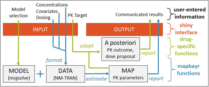
Workflow of a Shiny web app to perform therapeutic drug monitoring with maximum a posteriori Bayesian estimation performed by mapbayr. Data format, parameter estimation, and estimation report are common whatever the drug and can be assumed by mapbayr functions (in blue). Computation of a specific a posteriori outcome and forecast of a dose adaptation is specific to the drug or protocol (in green). Arguments can be passed through a Shiny app (in red) so that the user enters information through a convenient interface. MAP, maximum a posteriori; PK, pharmacokinetics

Validation process

The validation process consisted of comparing the ${\eta }_i$ estimations given by NONMEM and mapbayr for a large number of simulated patients, with a wide variety of models, dosing schedules, and sampling procedures.

Test models

A total of 35 test models were investigated as summarized in Table 1. The default model was a monocompartmental model with first‐order absorption and elimination. The IIV was set as log‐normal with ${\omega }_k^2$ = 0.2 on three parameters (and thus as many estimated ${\eta }_{\mathit{ik}}$ per individual): absorption rate constant (KA), volume of distribution (V), and clearance (CL). Residual error was coded as 20% proportional. The other models were derived from the default one, with additional estimation of parameters related to absorption (lag time, zero‐order infusion duration, and bioavailability), distribution (peripheral volume), or elimination (Michaelis–Menten constant [K_M] and maximum rate [V _MAX]). A model with time‐varying covariates was explored. Different residual error models were investigated (proportional, additive, mixed, and log‐additive) as well as simultaneously fitting two types of dependent variables (i.e., parent and metabolite). Finally, small or large values of IIV were tested (with ${\omega }_k^2$ ranging from 0.2 to 1 for every parameter) as well as very large IIV (${\omega }_k^2$ = 2) on one or multiple parameters. When applicable, all of these models were duplicated to allow for the administration either into a depot compartment (i.e., oral dosing) or in the central compartment (1‐h intravenous infusion).

TABLE 1.

Test models description

Model		Dosing	Estimated parameters	Model n°
Monocompartmental (default)		Oral	KA, CL, VC	1
		i.v. 1 h	(KA), CL, VC	2
Absorption	Lag time	Oral	KA, CL, VC, ALAG1	3
	Zero‐order in Central compartment	Oral	CL, VC, D2	4
	Zero‐order in Depot compartment	Oral	CL, VC, KA, D1	5
	Dual 0‐ and 1st orders (fixed FR)	Oral	CL, VC, KA, D2	6
	Dual 1st orders (fixed FR)	Oral	CL, VC, KA1, KA2	7
	Bioavailability	Oral	CL, VC, KA, F (logit)	8
Distribution	Bicompartmental	Oral	KA, CL, VC, VP	101
		i.v. 1 h	(KA), CL, VC, VP	102
Elimination	Michaelis–Menten (KM, VMAX)	Oral	KA, VC, KM, VMAX	201
		i.v. 1 h	(KA), VC, KM, VMAX	202
	CL + Michaelis–Menten (KM)	Oral	KA, CL, VC, KM	203
		i.v. 1 h	(KA), CL, VC, KM	204
	CL + Michaelis–Menten (VMAX)	Oral	KA, CL, VC, VMAX	205
		i.v. 1 h	(KA), CL, VC, VMAX	206
	CL + Michaelis–Menten (KM, VMAX)	Oral	KA, CL, VC, KM, VMAX	207
		i.v. 1 h	(KA), CL, VC, KM, VMAX	208
Time‐Varying Covariates	Time‐varying CL	Oral	KA, CL, VC	301
		i.v. 1 h	(KA), CL, VC	302
Residual Error Model	Metabolite	Oral	KA, CL, VC, CLmet, VCmet	401
		i.v. 1 h	(KA), CL, VC, CLmet, VCmet	402
	Additive	Oral	KA, CL, VC	403
		i.v. 1 h	(KA), CL, VC	404
	Mixed	Oral	KA, CL, VC	405
		i.v. 1 h	(KA), CL, VC	406
	Log‐additive	Oral	KA, CL, VC	407
		i.v. 1 h	(KA), CL, VC	408
Inter‐individual Variability	0.4 (63%) on KA, CL, VC	Oral	KA, CL, VC	501
	0.6 (77%) on KA, CL, VC	Oral	KA, CL, VC	502
	0.8 (89%) on KA, CL, VC	Oral	KA, CL, VC	503
	1 (100%) on KA, CL, VC	Oral	KA, CL, VC	504
	2 on CL, 0.2 on KA, VC	Oral	KA, CL, VC	511
	2 on CL, KA, 0.2 on VC	Oral	KA, CL, VC	512
	2 (141%) on CL, KA, VC	Oral	KA, CL, VC	513

Non‐identifiable KA estimated in intravenous administration context are in parentheses.

Abbreviations: ALAGx, lag time in compartment x; CL, clearance; CL_met, clearance of metabolite; Dx, infusion rate in compartment x; F, bioavailability constant; FR, fraction in depot compartment; i.v. 1 h, intravenous 1‐hour infusion; KA, absorption rate; K_M, Michaelis–Menten constant; VC, central volume of distribution; VC_met, central volume of metabolite; V_MAX, maximum rate; VP, peripheral volume of distribution.

For each model, 4000 individuals were attributed random values of ${\eta }_i$ and dispatched in four cohorts with a combination of administration (single or multiple dosing) and observation (sparse or rich sampling) schedules (Table 2). Doses of 10, 30, 60, 80 or 120 mg were given in each cohort (i.e., 200 individuals per dose level). Concentrations were simulated in mrgsolve, and a random proportional error of 10% was added. Null concentrations were excluded from the analysis (MDV = 1), and non‐null concentrations lower than 0.1 μg/ml were censored to this value. An example of a model code (mapbayr and NONMEM) and associated data are provided in the Supplementary Materials.

TABLE 2.

Test data description

Cohort	Administration times	Observations
Single dose, rich sampling	0 h	1 ± 0.5 h
		4 ± 1 h
		8 ± 2 h
		24 ± 6 h
Single dose, sparse sampling	0 h	24 ± 10 h
Multiple doses, rich sampling	0, 72, 96, 120, 144, 168, 192 and 216 h	215 ± 0.5 h
		217 ± 1 h
		220 ± 1 h
		224 ± 2 h
Multiple doses, sparse sampling	0, 72, 96, 120, 144, 168, 192 and 216 h	240 ± 10 h

Real models

In addition to the test models, the performance of mapbayr was assessed on seven real models corresponding to published clinical studies for which a population PK model was developed and fully reported. They combine different features separately explored with test models. Data were generated in accordance with the drug administration schedules and sampling strategies used in the context of TDM with n = 1000 individuals. In addition, a variable corresponding to the routinely monitored PK outcome was computed with both NONMEM and mapbayr: last dose of a 3‐day schedule to reach a total AUC of 24 mg·min/ml for carboplatin ³² ; AUC at steady state between two doses (AUC_τ,SS) for ibrutinib ³³ , ³⁴ ; trough concentration at steady state for cabozantinib, ³⁵ pazopanib, ³⁶ and voriconazole ³⁷ ; sum of parent drug and metabolite trough concentration for sunitinib and N‐desethyl‐sunitinib ³⁸ ; and time to reach a concentration below 0.2 μmol/L for methotrexate. ³⁹ A detailed description of these models and the related data are provided in Table 3.

TABLE 3.

Real models and data description

N°	Model/drug	Doses	Features	Sampling	Outcome
901	Carboplatin 32	Single 1‐h i.v. Amt: 500, 750, 1000, 1250 mg	Linear bicompartmental model with proportional error (three parameters)	0.95 ± 0.1 h 2 ± 0.2 h 5 ± 0.3 h	Remaining dose to obtain an AUC of 24 mg·min/ml
911	Ibrutinib 33 , 34	Multiple oral (one dose, SS = 1, ii = 24, then one dose at time 24h, SS = 0). Amt: 140, 280, 420, 560 mg	Oral absorption with zero‐order and lag time, parent + metabolite (12 parameters)	23.5 ± 0.5 h 26 ± 0.5 h 28 ± 0.5 h	AUCτ,SS
921	Pazopanib 36	Multiple oral (addl = 27, ii = 24). Amt: 200, 400, 800, 1000 mg and mixed	Dual first‐order absorption with time‐varying and dose‐varying variability (time‐varying covariate). IOV on relative bioavailability. Mixed residual error (six parameters)	330 ± 5 h (Cycle 1) 672 ± 10 h (Cycle 2)	Cmin
931	Cabozantinib 35	Multiple oral (addl = 27, ii = 24). Amt: 20, 40, 60 mg and mixed	Dual first‐order and zero‐order absorption, dose‐dependent absorption rate, exponential residual error (four parameters)	672 ± 10 h	Cmin
941	Sunitinib 38	Multiple oral (addl = 13, ii = 24). Amt: 25, 37.5, 50 mg and mixed	Parent + metabolite, nonlinear PK (concentration‐dependent clearance) (four parameters)	336 ± 10 h	Sum Cmin Suni + NDSuni
951	Methotrexate 39	Single 6 h‐i.v. Amt: 2000, 5000, 8000, and 10000 mg	Linear bicompartmental model, IOV on clearance, and proportional error (six parameters)	24 ± 3 h 48 ± 3 h At Cycle 1 and Cycle 2	Time to reach a concentration of 0.2 μM
962	Voriconazole (adult patients and oral dosing) 37	Multiple oral (two 400 mg doses, ii = 12, then 200 mg, addl = 11, ii = 12)	Linear and time‐varying Michaelis–Menten elimination, with very large IIV (variance 1.39). Box‐Cox transformed bioavailability. Exponential residual error (seven parameters)	72 ± 5 h 168 ± 5 h	Cmin

Abbreviations: addl, additional given dose; Amt, amount; AUC, area under the curve of concentrations versus time; AUC_τ,SS, AUC at steady state between two doses; Cmin, trough concentration; ii, interdose interval in hours; IIV, inter‐individual variability; IOV, interoccasion variability; i.v., intravenous; NDSuni, N‐desethyl‐sunitinib; PK, pharmacokinetics; SS, steady state; Suni, sunitinib.

Analysis

Parameters were estimated with mapbayr and NONMEM with software specifications mentioned in the Supplementary Materials. The performance of mapbayr was assessed by computing the maximum absolute difference on ${\widehat{\eta }}_{\mathit{ik}}$ obtained with mapbayr (${\widehat{\eta }}_{ik,MBR}$) and NONMEM (${\widehat{\eta }}_{ik,NM}$) for every individual as follows:

$${\mathrm{\Delta }\widehat{\eta }}_{\mathit{ik}}=\left|{\widehat{\eta }}_{ik,MBR}‐{\widehat{\eta }}_{ik,NM}\right|,$$

$${\mathrm{\Delta }\widehat{\eta }}_i=\max \left({\mathrm{\Delta }\widehat{\eta }}_{\mathit{ik}}\right),$$

These values have no unit. However, provided that individual PK parameters (${\theta }_i$) were log‐normally distributed around a typical value (${\theta }_{\mathit{TV}}$) such as ${\theta }_i={\theta }_{\mathit{TV}}\bullet \exp ({\eta }_i)$, the maximum error on parameter value could be defined by ${\mathrm{\Delta }\widehat{\theta }}_i=\frac{{\theta }_{i,\mathrm{MBR}}‐{\theta }_{i,\mathrm{NM}}}{{\theta }_{i,\mathrm{NM}}}=\exp \left({\mathrm{\Delta }\widehat{\eta }}_i\right)‐1$. Thus, performance thresholds could be defined accordingly. If ${\mathrm{\Delta }\widehat{\eta }}_i$ was lower than 0.001, estimation was considered excellent because the impact on parameter values would be negligible (${\mathrm{\Delta }\widehat{\theta }}_i$ < 0.1%). If ${\mathrm{\Delta }\widehat{\eta }}_i$ was higher than 0.095, the estimation was considered discordant (${\mathrm{\Delta }\widehat{\theta }}_i$ > 10%). In other cases, estimation was considered acceptable. The same classification was applied to the absolute error on the PK outcomes measured with the real models.

Although NONMEM was considered as the reference that should return the best estimate of ${\eta }_i$, this assumption was challenged by comparing the ${\mathrm{OFV}}_i$ returned by both software. However, the actual ${\mathrm{OFV}}_i$ returned by NONMEM into the .phi file includes a constant term that is missing in the formula in the "MAP Bayesian estimation" Section. Thus, the direct comparison of NONMEM’s ${\mathrm{OFV}}_i$ to mapbayr's ${\mathrm{OFV}}_i$ (${\mathrm{OFV}}_{i,\mathrm{MBR}}$) could not be performed. A NONMEM‐like ${\mathrm{OFV}}_i$ (${\mathrm{OFV}}_{i,\mathrm{NM}‐\mathrm{like}})$ was recomputed using ${\widehat{\eta }}_{i,\mathrm{NM}}$ with the same formula as in Section 2.1 to ensure comparison to ${\text{OFV}}_{i,\text{MBR}}$.

RESULTS

Package features

mapbayr strongly relies on features provided by mrgsolve, a package to perform simulations from PK or PK/PD models. Notably, mrgsolve was intentionally designed to be similar to NONMEM in terms of model coding, with code blocks written in R/C++ with a syntax close to that of NONMEM’s FORTRAN. Thus, if a user is familiar with NONMEM, it is rather straightforward to transpose a model into mrgsolve, unlike other available packages such as RxODE or nlmixr. ²¹ , ⁴⁰ mrgsolve also accepts data passed into a NM‐TRAN format.

Overall, mapbayr was built around mrgsolve to perform MAP‐BE from a mrgsolve model and includes the following features:

• MAP‐BE with R only. An additional software such as NONMEM, or MATLAB is not needed.

• MAP‐BE with every type of structural model accepted in mrgsolve, including time‐varying covariates and nonlinear PK.

• MAP‐BE with any random effects on parameters, including interoccasion variability (IOV) and correlations between IIV terms.

• MAP‐BE with proportional, additive, mixed, and exponential residual error models. There is no need to transform the data or to pass additional arguments.

• MAP‐BE with dependent variables defined in multiple compartments, such as parent drug and its metabolite.

However, procedures available in NONMEM that do not rely on a unique minimization of the likelihood with respect to the etas, such as mixture models, are not natively supported by mapbayr.

In practice, estimations are performed with a single function that only requires two arguments: model and data.

my_model <‐ mread(“path/to/my/model/code.cpp”) # a mrgsolve model

my_data <‐ read.csv(“path/to/my/dataset.csv”) #a NM‐TRAN dataset

my_est <‐ mapbayest(my_model, my_data)

Additional features also include functions to enter information about administrations and observations so that the data set is automatically formatted to NM‐TRAN format as well as methods to plot and summarize the results of estimation. These functions deal with the burden of formatting data and plotting results so that the programmer can focus on functions specific to the drug and TDM protocol. To that extent, model and estimation objects are meant to be exploited by functions coded by the user to derive the PK outcome of interest (AUC, simulated concentrations, dose proposal, etc.) and to be included into a Shiny application (Figure 1).

Validation of test models

Over the 140,000 estimations performed with both NONMEM and mapbayr on test models, median ${\mathrm{\Delta }\widehat{\theta }}_i$ was 0.0004%, and 98% of estimations were excellent (${\mathrm{\Delta }\widehat{\theta }}_i$ < 0.1%), 0.5% were acceptable, and 1.5% were discordant (${\mathrm{\Delta }\widehat{\theta }}_i$ > 10%) (Figure 2). Excellent performances were found in particular for the default models (Runs 1 and 2), models with bicompartmental distribution (101 and 102), time‐varying covariates (301 and 302), and alternative residual error models (401 to 408).

FIGURE 2.

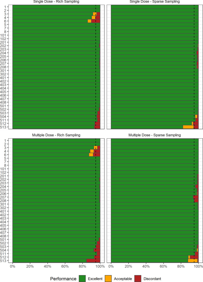
Performance with 35 test models and four dosing/sampling regimens on parameter estimation. Each line represents 1000 estimations with an associated performance score: excellent if ${\mathrm{\Delta }\widehat{\theta }}_i$ < 0.1%, discordant if ${\mathrm{\Delta }\widehat{\theta }}_i$ > 10%, and acceptable in between. Dashed line indicates 95th percentile

However, in some situations, a higher percentage of individuals with discordant estimations was observed. The highest discordances were seen with Runs 3, 4, and 6 with rich sampling; among these 6000 individuals, 371 (6.2%) had discordant estimates. These models needed an estimation of lag time (Run 3) or a zero‐order infusion duration from extravascular compartment (Runs 4 and 6), whereas no discrepancy was observed when bioavailability (Run 8) or first‐order absorption constants (Runs 7 and 8) had to be estimated. Among these 371 patients, ${\mathrm{OFV}}_{i,\mathrm{MBR}}$ was lower than ${\mathrm{OFV}}_{i,\mathrm{NM}‐\mathrm{like}}$ in 225 patients (61%), suggesting that the actual ${\widehat{\eta }}_i$ was more likely to be found with mapbayr rather than NONMEM (Figure 3). Thus, mapbayr was probably worse than NONMEM in only 146 of the 6000 individuals (2.4%), and differences on parameter estimates were mainly observed on the absorption parameters (lag time [LAG] or infusion duration [DUR]) rather than on apparent CL, with median ${\mathrm{\Delta }\widehat{\theta }}_{i,k=\mathrm{LAG}\mathrm{or}\mathrm{DUR}}$ = 24% and ${\mathrm{\Delta }\widehat{\theta }}_{i,k=\mathrm{CL}}$ = 1.6%, respectively.

FIGURE 3.

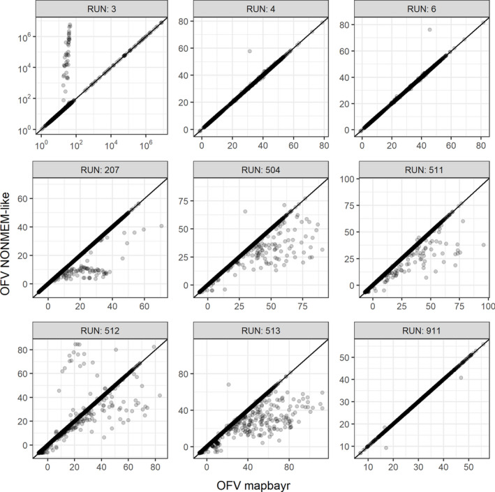
OFVs at maximum likelihood for mapbayr and NONMEM. They were aligned on the identity line for the majority of individuals (4000 per run). Discrepancies were in favor of mapbayr for Run 3 (lag time), mainly in favor of NONMEM for Runs 207 (Michaelis–Menten elimination) and 504–513 (large inter‐individual variability), and balanced for Runs 4, 6 (infusion duration), and 911 (ibrutinib). One out‐of‐bound value is omitted in Run 911. OFV, objective function value

For models with a nonlinear Michaelis–Menten elimination (Runs 201 to 208), 2.5% of estimations were discordant in the “multiple doses + sparse sampling” setup. This rate was up to 6.1% with Model 207, when KA, VC, CL, V_MAX, and K_M had to be estimated from a single point at steady state. Unlike Runs 3, 4, and 6, ${\mathrm{OFV}}_{i,\mathrm{MBR}}$ was always the same or higher than ${\mathrm{OFV}}_{i,\mathrm{NM}‐\mathrm{like}}$ (Figure 3), suggesting that discordant estimates returned by mapbayr were probably less correct compared with NONMEM’s.

For Runs 501 to 513, the percentage of individuals with discordant estimations increased proportionally to the IIV value set in the model. Focusing on the “multiple doses + rich sampling” setting (Figure 2), a maximum of 15% discordances was observed with Model 513 (${\omega }_k^2$ = 2 on every parameter). The percentage of discordant estimations was not higher than 7% if ${\omega }_k^2$ was equal to 2 on certain parameters only (Runs 511 and 512) or if ${\omega }_k^2$ was less or equal to 1 on all parameters (from 501 to 504). ${\mathrm{OFV}}_{i,\mathrm{MBR}}$ was often higher than or equal to ${\mathrm{OFV}}_{i,\mathrm{NM}‐\mathrm{like}}$ (Figure 3). Because simulations were performed by sampling from large parameter distributions, we hypothesized that a substantial number of PK profiles were probably abnormal and reperformed the analysis after the exclusion of PK profiles with concentrations censored to 0.1 µg/ml. All sampling/dosing cohorts combined, a maximum of 4.9% discordance was observed (Run 513). Focusing on a specific cohort, only 3/28 returned a discordance rate higher than 5%, all with at least two ${\omega }_k^2$ = 2 (Table S1).

Validation of the real models

For the seven real models, the performance of mapbayr was satisfactory with overall 97.3% and 99.3% of excellent estimations for PK parameters and PK outcomes, respectively (Figure 4). The run with ibrutinib (911), a complex model with 12 parameters to estimate, returned a median ${\mathrm{\Delta }\widehat{\theta }}_i$ of 0.05%, compared with 0.0004% for the test models. Despite this genuine loss in performance (about 150 times less precise), estimations were satisfactory in terms of parameters (84.3% excellent and only 0.7% discordant) and in terms of PK outcome with only 5/1000 individuals with an error >10% on AUC_τ,SS. For methotrexate (Run 951), the predicted time to reach a concentration below 0.2 μM was discordant in only 6/1000 patients, corresponding to outlier situations when concentration was already lower than 0.2 μM at the first sample, or concentrations higher at 48 h than 24 h postdose. For voriconazole, trough concentration predictions were discordant for 6/1000 patients only, despite the structural complexity of the model and the very large variance set on Michaelis–Menten elimination parameters (shared eta with ${\omega }_k^2$ = 1.39). For the other real models, 100% rates of “excellent” estimation (difference <0.1%) between mapbayr and NONMEM were achieved. The proposed dose to reach an AUC of 24 mg·min/ml for carboplatin (Run 901) ranged from 0 to 6000 mg. The steady‐state trough concentrations of pazopanib, cabozantinib, and sunitinib + NDsunitinib were estimated identically by both software (median values 19 mg/L, 0.66 mg/L, and 45 mg/L, respectively), which would lead to an identical dose adaptation if used in the context of TDM.

FIGURE 4.

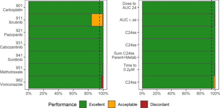
Performance with seven real models on parameter (left) and specific PK outcome (right) estimation. Dashed line indicates 95th percentile. AUC, area under the curve of concentrations versus time; AUC_τ,SS, AUC at steady state between two doses; C24ss, trough concentration at steady state

DISCUSSION

A package that enables the MAP‐BE of PK parameters in R was developed, and its prediction capacity was validated against the gold‐standard software NONMEM.

The performance of mapbayr is overall equivalent to NONMEM’s for a wide variety of test models. Most of the discrepancies were observed when large IIVs were investigated (Runs 501 to 513), notably when ${\omega }_k^2$ = 2 on all parameters (Run 513). This is probably because large variances cause a flatter surface of the likelihood, which makes minimization difficult. However, in real‐life situations, such high discordance rates are unlikely because the current test scenarios probably returned abnormal PK profiles due to sampling from very large distributions for a majority of parameters. Indeed, the reanalysis of test model data without censored concentrations (0.1 µg/ml) returned more acceptable results (Table S1). In real life, very large variances (>1) on several parameters and such aberrant profiles seem highly unlikely. For the voriconazole model, excellent rates of concentration estimation were observed despite a variance higher than one on elimination parameters (Figure 3). Overall, for a few individuals, mapbayr is genuinely outperformed by NONMEM when MAP‐BE is performed with large IIV variances (${\omega }_k^2$ > 1) on several estimable parameters. In those rare cases, mapbayr use remains possible, although it would be advisable to perform a validation versus NONMEM from simulated data with the expected dosing/sampling strategy (i.e., “real‐models” setting).

Several discrepancies were also seen when lag time or infusion duration were estimated, but the exploration of ${\mathrm{OFV}}_i$suggested that estimates from mapbayr were often more likely than those of NONMEM. This might be because lag times can create big discontinuities in ${\mathrm{OFV}}_i$, due to the prediction of null concentrations if a lag time is greater than an observation time. For instance, if a concentration is observed at time t = 0.5 h, and a lag time of 1 h (typical value) is tested by the optimization algorithm, an extremely high ${\mathrm{OFV}}_i$ would be returned whatever the values of the other parameters (CL, V) because the dose is still missing in the system. This situation leads to local minimums, which is why ${\mathrm{OFV}}_i$ around 10⁴ to 10⁷ were observed for some patients in Run 3, whereas the global minimum was expected around 10¹ or 10² (Figure 3). Thus, for some patients, when lag time and infusion duration had to be estimated, mapbayr could outdo NONMEM provided that our own computation of ${\mathrm{OFV}}_{i,\mathrm{NM}‐\mathrm{like}}$ is not false.

However, in other situations (Michaelis–Menten elimination, large IIV), differences between mapbayr and NONMEM were often in favor of the latter. The different algorithms used (L‐BFGS‐B vs. BFGS) and their associated settings probably explain these discrepancies in estimation. The hypothesis of differences in concentration prediction that would distort the computation of ${\mathrm{OFV}}_i$ is less likely. Both software use the LSODA ODE solver to predict concentrations, and its C++ implementation in mrgsolve was found to be consistent to NONMEM’s given the performances provided by mrgsolve. ⁴¹

Estimation of parameters for real models (901 and more) returned a high percentage of patients with excellent performance despite a higher complexity in both structural and error models. This proves the estimation returned by mapbayr (${\widehat{\eta }}_{i,\mathrm{MBR}}$) is as reliable than the NONMEM estimate (${\widehat{\eta }}_{i,\mathrm{NM}}$). However, it cannot inform us regarding the ability to return the actual value of ${\eta }_i$. Indeed, although any PK model reported in the literature could theoretically be coded within mapbayr to perform MAP‐BE and derive an individualized dose, the Bayesian estimation design must have been previously validated. ⁴² First, the residual error defined in the PK model must be small enough to correctly estimate PK parameters and avoid $\eta$‐shrinkage on key parameters (to be defined depending on the clinical applications). ⁴³ Second, the sampling strategy must have been previously validated to make sure that parameter estimation is precise enough, especially when very sparse sampling is used in the context of a routine TDM. These questions of design optimality can be addressed with specific software (notably the R packages PFIM ⁴⁴ or PopED ⁴⁵ ) or more pragmatic approaches such as validation on a clinical data set.

There was no proper comparison of run times of mapbayr versus NONMEM; however, there is no doubt that the first is slower because it was mainly written in R language, which is known to be slower than FORTRAN. Computation time increased with the number of parameters estimated: from milliseconds per individual for simple models with three to four parameters, to a couple of seconds for complex models with 12 parameters such as ibrutinib. Hence, maybayr's run times are fully compatible with routine use in clinical practice.

Although some difficulties in the generalization of MIPD remain to be overcome (e.g., regulatory aspects that may require registration of these tools as medical devices in some countries), ⁴⁶ this tool will undoubtedly be of great interest for clinically oriented researchers.

From the estimated PK parameters, the user can derive PK outcomes of interest with standard R programming. Using simple arithmetic functions, an AUC can be derived from (oral) CL and dose. Moreover, using the mrgsolve framework, individual concentrations can be predicted at any times assumed relevant by the user. For example, the concentration of a tyrosine kinase inhibitor could be predicted exactly 24 h after the last intake to compare it to an efficacy threshold if sampling time has not been respected. ⁴⁷ The time at which a drug concentration reaches a given threshold can also be predicted to infer the time to next administration or to decide on a patient's discharge (e.g., for methotrexate). Alternative dosing schedules can also be simulated from a posteriori individual PK parameters to predict dose adjustment and manage drug exposure. Several examples of shiny applications that include these procedures are provided in a dedicated repository at https://github.com/FelicienLL/mapbayr‐shiny.

Currently, estimations performed by mapbayr are only maximum a posteriori, which means most probable parameter values without taking uncertainties of estimation into account. Recently, Bayesian data assimilation methods have been suggested to overcome this limitation in the context of TDM. ⁴⁸ Future versions of mapbayr could implement procedures based on the Fisher information matrix or on sampling from the posterior distribution. As a free and open‐source package, mapbayr is developed on Github and available on Comprehensive R Archive Network. Users are welcome to suggest features, report bugs, and participate in development at https://github.com/FelicienLL/mapbayr.

In conclusion, instead of providing a ready‐made application that would only be applicable for a limited number of users and clinical situations and mimic existing MIPD software, we developed a general tool to deal with the most sensitive step of model‐based TDM: the MAP‐BE. With mapbayr, anyone familiar with R can transpose any of his/her own models into a Shiny web application to perform TDM with a reliable MAP‐BE of individual parameters without external modeling software. We hope this approach will help the development of MIPD, especially in less‐considered therapeutic areas such as oncology.

CONFLICT OF INTEREST

The authors declared no competing interests for this work.

AUTHOR CONTRIBUTIONS

F.L.L., F.P., F.T., E.C., and M.W.K. wrote the manuscript. F.L.L., E.C., and M.W.K. designed the research. F.L.L. performed the research. F.L.L. and M.W.K. analyzed the data. F.L.L. contributed new analytical tools.

Supporting information

Table S1

Supplementary Material

Le Louedec F, Puisset F, Thomas F, Chatelut É, White‐Koning M. Easy and reliable maximum a posteriori Bayesian estimation of pharmacokinetic parameters with the open‐source R package mapbayr. CPT Pharmacometrics Syst Pharmacol. 2021;10:1208–1220. 10.1002/psp4.12689

REFERENCES

- 1. Definitions of TDM &CT. https://www.iatdmct.org/about‐us/about‐association/about‐definitions‐tdm‐ct.html. Accessed June 21, 2021.
- 2. Kang J‐S, Lee M‐H. Overview of therapeutic drug monitoring. Korean J Intern Med. 2009;24:1‐10. [DOI] [PMC free article] [PubMed] [Google Scholar]
- 3. Ting LSL, Villeneuve E, Ensom MHH. Beyond cyclosporine: A systematic review of limited sampling strategies for other immunosuppressants. Ther Drug Monit. 2006;28:419‐430. [DOI] [PubMed] [Google Scholar]
- 4. Chatelut E, Pivot X, Otto J, et al. A limited sampling strategy for determining carboplatin AUC and monitoring drug dosage. Eur J Cancer. 2000;36:264‐269. [DOI] [PubMed] [Google Scholar]
- 5. Tranchand B, Amsellem C, Chatelut E, et al. A limited‐sampling strategy for estimation of etoposide pharmacokinetics in cancer patients. Cancer Chemotherapy Pharmacology. 1999;43:316‐322. [DOI] [PubMed] [Google Scholar]
- 6. van Kuilenburg ABP, Häusler P, Schalhorn A, et al. Evaluation of 5‐fluorouracil pharmacokinetics in cancer patients with a C. 1905+1G>A mutation in DPYD by means of a Bayesian limited sampling strategy. Clin Pharmacokinet. 2012;51:163‐174. [DOI] [PubMed] [Google Scholar]
- 7. Wicha SG, Märtson A‐G, Nielsen EI, et al. From therapeutic drug monitoring to model‐informed precision dosing for antibiotics. Clin Pharm Therap. 2021;109:928‐941. [DOI] [PubMed] [Google Scholar]
- 8. Sheiner LB, Rosenberg B, Melmon KL. Modelling of individual pharmacokinetics for computer‐aided drug dosage. Comput Biomed Res. 1972;5:411‐459. [DOI] [PubMed] [Google Scholar]
- 9. Beal SL, Sheiner LB, Boeckmann A, et al. NONMEM Users Guides . San Francisco: NONMEM Project Group, University of California; 1992. [Google Scholar]
- 10. BestDose Software. http://www.lapk.org/bestdose.php. Accessed June 21, 2021.
- 11. InsightRX–Precision Dosing Done Right. https://www.insight‐rx.com/. Accessed June 21, 2021.
- 12. Precise PK. A leading therapeutic drug monitoring software for model‐based Bayesian precision dosing. https://precisepk.com/. Accessed June 21, 2021.
- 13. Kantasiripitak W, Van Daele R, Gijsen M, et al. Software tools for model‐informed precision dosing: how well do they satisfy the needs? Front Pharmacol. 2020;11:620. [DOI] [PMC free article] [PubMed] [Google Scholar]
- 14. Dijkman SC, Wicha SG, Danhof M, et al. Individualized dosing algorithms and therapeutic monitoring for antiepileptic drugs. Clin Pharmacol Ther. 2018;103:663‐673. [DOI] [PubMed] [Google Scholar]
- 15. Rousseau A, Marquet P, Debord J, et al. Adaptive control methods for the dose individualisation of anticancer agents. Clin Pharmacokinet. 2000;38:315‐353. [DOI] [PubMed] [Google Scholar]
- 16. R Core Team . R: A language and environment for statistical computing. https://www.R‐project.org/. Accessed June 21, 2021.
- 17. Shiny. https://shiny.rstudio.com/. Accessed June 21, 2021.
- 18. Wojciechowski J, Hopkins AM, Upton RN. Interactive pharmacometric applications using R and the shiny package. CPT Pharmacometrics Syst Pharmacol. 2015;4:e00021. [DOI] [PMC free article] [PubMed] [Google Scholar]
- 19. Okour M. DosePredict: A shiny application for generalized pharmacokinetics‐based dose predictions. J Clin Pharmacol. 2020;60:1502‐1508. [DOI] [PubMed] [Google Scholar]
- 20. Wicha SG, Kees MG, Solms A, et al. TDMx: A novel web‐based open‐access support tool for optimising antimicrobial dosing regimens in clinical routine. Int J Antimicrob Agents. 2015;45:442‐444. [DOI] [PubMed] [Google Scholar]
- 21. Fidler M, Wilkins JJ, Hooijmaijers R, et al. Nonlinear mixed‐effects model development and simulation using nlmixr and related R Open‐Source Packages. CPT: Pharmacom Sys. Pharmacol. 2019;8:621‐633. [DOI] [PMC free article] [PubMed] [Google Scholar]
- 22. Comets E, Lavenu A, Lavielle M. Parameter estimation in nonlinear mixed effect models using saemix, an R implementation of the SAEM algorithm. J Stat Softw. 2017;80:1‐41. [Google Scholar]
- 23. Wang W, Hallow KM, James DA. A tutorial on RxODE: simulating differential equation pharmacometric models in R. CPT Pharmacometrics Syst Pharmacol. 2016;5:3‐10. [DOI] [PMC free article] [PubMed] [Google Scholar]
- 24. Elmokadem A, Riggs MM, Baron KT. Quantitative systems pharmacology and physiologically‐based pharmacokinetic modeling with mrgsolve: a hands‐on tutorial. CPT Pharmacometrics Syst Pharmacol. 2019;8:883‐893. [DOI] [PMC free article] [PubMed] [Google Scholar]
- 25. Baron KT, Gillespie B, Margossian C, et al. mrgsolve: simulate from ODE‐based models. https://CRAN.R‐project.org/package=mrgsolve. Published 2020. Accessed June 21, 2021.
- 26. Kang D, Bae K‐S, Houk BE, et al. Standard error of empirical bayes estimate in NONMEM® VI. Korean J Physiol Pharmacol. 2012;16:97. [DOI] [PMC free article] [PubMed] [Google Scholar]
- 27. Kim M‐G, Yim D‐S, Bae K‐S. R‐based reproduction of the estimation process hidden behind NONMEM® Part 1: first‐order approximation method. Transl Clin Pharmacol. 2015;23:1. [DOI] [PMC free article] [PubMed] [Google Scholar]
- 28. Bae K‐S, Yim D‐S. R‐based reproduction of the estimation process hidden behind NONMEM® Part 2: First‐order conditional estimation. Transl Clin Pharmacol. 2016;24:161. [DOI] [PMC free article] [PubMed] [Google Scholar]
- 29. Generate MAP Bayes parameter estimates. https://mrgsolve.github.io/blog/map_bayes.html. Accessed June 21, 2021.
- 30. Bauer RJ. NONMEM tutorial part I: Description of commands and options, with simple examples of population analysis. CPT Pharmacometrics Syst Pharmacol. 2019;8:525‐537. [DOI] [PMC free article] [PubMed] [Google Scholar]
- 31. Nash JC, Varadhan R, Grothendieck G. optimx: expanded replacement and extension of the “optim” function. https://CRAN.R‐project.org/package=optimx. Published 2020. Accessed March 23, 2021.
- 32. Moeung S, Chevreau C, Broutin S, et al. Therapeutic drug monitoring of carboplatin in high‐dose protocol (TI‐CE) for advanced germ cell tumors: Pharmacokinetic results of a phase II multicenter study. Clin Cancer Res. 2017;23:7171‐7179. [DOI] [PubMed] [Google Scholar]
- 33. Gallais F, Ysebaert L, Despas F, et al. Population pharmacokinetics of ibrutinib and its dihydrodiol metabolite in patients with lymphoid malignancies. Clin Pharmacokinet. 2020;59:1171‐1183. [DOI] [PubMed] [Google Scholar]
- 34. Le Louedec F, Gallais F, Thomas F, et al. Limited sampling strategy for determination of ibrutinib plasma exposure, Joint analyses with metabolite data. Pharmaceuticals (Basel). 2021;14. [DOI] [PMC free article] [PubMed] [Google Scholar]
- 35. Nguyen L, Chapel S, Tran BD, et al. Updated population pharmacokinetic model of cabozantinib integrating various cancer types including hepatocellular carcinoma. J Clin Pharmacol. 2019;59:1551‐1561. [DOI] [PMC free article] [PubMed] [Google Scholar]
- 36. Yu H, van Erp N, Bins S, et al. Development of a pharmacokinetic model to describe the complex pharmacokinetics of Pazopanib in cancer patients. Clin Pharmacokinet. 2016;56:293‐303. [DOI] [PubMed] [Google Scholar]
- 37. Friberg LE, Ravva P, Karlsson MO, et al. Integrated population pharmacokinetic analysis of voriconazole in children, adolescents, and adults. Antimicrob Agents Chemother. 2012;56:3032‐3042. [DOI] [PMC free article] [PubMed] [Google Scholar]
- 38. Yu H, Steeghs N, Kloth JSL, et al. Integrated semi‐physiological pharmacokinetic model for both sunitinib and its active metabolite SU12662. Br J Clin Pharmacol. 2015;79:809‐819. [DOI] [PMC free article] [PubMed] [Google Scholar]
- 39. Faltaos DW, Hulot JS, Urien S, et al. Population pharmacokinetic study of methotrexate in patients with lymphoid malignancy. Cancer Chemother Pharmacol. 2006;58:626‐633. [DOI] [PubMed] [Google Scholar]
- 40. Schoemaker R, Fidler M, Laveille C, et al. Performance of the SAEM and FOCEI algorithms in the open‐source, nonlinear mixed effect modeling tool nlmixr. CPT Pharmacometrics Syst Pharmacol. 2019;8:923‐930. [DOI] [PMC free article] [PubMed] [Google Scholar]
- 41. GitHub. mrgsolve/nmtests . https://github.com/mrgsolve/nmtests. Accessed June 21, 2021.
- 42. van der Meer AF, Marcus MAE, Touw DJ, et al. Optimal sampling strategy development methodology using maximum A posteriori Bayesian estimation. Ther Drug Monit. 2011;33:133‐146. [DOI] [PubMed] [Google Scholar]
- 43. Savic RM, Karlsson MO. Importance of shrinkage in empirical bayes estimates for diagnostics: problems and solutions. AAPS J. 2009;11:558‐569. [DOI] [PMC free article] [PubMed] [Google Scholar]
- 44. Dumont C, Lestini G, Le Nagard H, et al. PFIM 4.0, an extended R program for design evaluation and optimization in nonlinear mixed‐effect models. Comput Methods Programs Biomed. 2018;156:217‐229. [DOI] [PubMed] [Google Scholar]
- 45. Nyberg J, Ueckert S, Strömberg EA, et al. PopED: an extended, parallelized, nonlinear mixed effects models optimal design tool. Comput Methods Programs Biomed. 2012;108:789‐805. [DOI] [PubMed] [Google Scholar]
- 46. Kluwe F, Michelet R, Mueller‐Schoell A, et al. Perspectives on model‐informed precision dosing in the digital health era: challenges, opportunities, and recommendations. Clin Pharmacol Ther. 2021;109:29‐36. [DOI] [PubMed] [Google Scholar]
- 47. Leenhardt F, Viala M, Tosi D, et al. Therapeutic Bayesian monitoring of sunitinib in two patients with impaired absorption or elimination. J Clin Pharm Ther. 2021;46(4):1182‐1184. [DOI] [PubMed] [Google Scholar]
- 48. Maier C, Hartung N, Wiljes J, et al. Bayesian data assimilation to support informed decision making in individualized chemotherapy. CPT Pharmacometrics Syst Pharmacol. 2020;9:153‐164. [DOI] [PMC free article] [PubMed] [Google Scholar]
Associated Data
This section collects any data citations, data availability statements, or supplementary materials included in this article.
Supplementary Materials