A Multimodal Computer-Aided Diagnostic System for Precise Identification of Renal Allograft Rejection: Preliminary Results

Abstract

Purpose:

Early assessment of renal allograft function post-transplantation is crucial to minimize and control allograft rejection. Biopsy—the gold standard—is used only as a last resort due to its invasiveness, high cost, adverse events (e.g., bleeding, infection, etc.), and the time for reporting. To overcome these limitations, a renal computer-assisted diagnostic (Renal-CAD) system was developed to assess kidney transplant function.

Methods:

The developed Renal-CAD system integrates data collected from two image-based sources and two clinical-based sources to assess renal transplant function. The imaging sources were the apparent diffusion coefficients (ADCs) extracted from 47 diffusion-weighted magnetic resonance imaging (DW-MRI) scans at 11 different b-values (b0, b50, b100, …, b1000 s/mm²), and the transverse relaxation rate (R2*) extracted from 30 blood oxygen level-dependent MRI (BOLD-MRI) scans at 5-different echo-times (TE = 2, 7, 12, 17, and 22 ms). Serum creatinine (SCr) and creatinine clearance (CrCl) were the clinical sources for kidney function evaluation. The Renal-CAD system initially performed kidney segmentation using the level-sets method followed by estimation of the ADCs from DW-MRIs and the R2* from BOLD-MRIs. ADCs and R2* estimates from 30 subjects that have both types of scans were integrated with their associated SCr and CrCl. The integrated biomarkers were then used as our discriminatory features to train and test a deep learning-based classifier; namely, stacked autoencoders (SAEs) to differentiate non-rejection (NR) from acute rejection (AR) renal transplants.

Results:

Using a leave-one-subject-out cross-validation approach along with SAEs, the Renal-CAD system demonstrated 93.3% accuracy, 90.0% sensitivity, and 95.0% specificity in differentiating AR from NR. Robustness of the Renal-CAD system was also confirmed by the area under the curve value of 0.92. Using a stratified 10-fold cross-validation approach, the Renal-CAD system demonstrated its reproduciblity and robustness by a diagnostic accuracy of 86.7%, sensitivity of 80.0%, specificity of 90.0% and AUC of 0.88.

Conclusion:

The obtained results demonstrate the feasibility and efficacy of accurate, non-invasive identification of AR at an early stage using the Renal-CAD system.

I. INTRODUCTION AND PURPOSE

Chronic kidney disease (CKD) is the ninth leading cause of mortality in the United States. Approximately, 15% of the population in the USA suffer from CKD with more than 700,000 patients diagnosed with end-stage renal disease (ESRD). Over $114 billion is spent annually on diagnosis and treatment of CKD or ESRD¹. Although renal transplantation provides the best outcome for ESRD patients, only 17,500 renal transplants are performed in the USA each year due to the paucity of donor organs^2,3. Significantly, 15%–27% of renal allograft patients are diagnosed with acute rejection (AR) within the first 5 years post-transplantation. AR of renal allografts has to be detected and treated promptly at an early stage, to minimize permanent damage and failure of the transplanted kidney^2,3. Given the dearth of living or cadaveric donors, routine clinical follow-up, assessment, and functionality evaluation of the renal allograft post-transplantation is crucial to minimize allograft loss⁴.

The diagnostic technique that is currently recommended by the National Kidney Foundation (NKF) for assessing renal allograft function is the glomerular filtration rate (GFR). The GFR has low sensitivity and is a late indicator for renal allograft dysfunction as major/noticeable changes can only be observed after>60% of renal allograft function is lost⁵. Renal biopsy, the gold standard, is used as a conclusive AR diagnostic tool. However, it cannot be used as a screening or early detection tool due to high invasiveness, high cost, long time for recovery/report, and associated adverse events (infection, bleeding, etc.). Therefore, there is a significant unmet clinical need for a non-invasive diagnostic tool that can provide a precise and early identification of AR renal allograft.

Recently, diffusion-weighted magnetic resonance imaging (DW-MRI)^6–11 and blood oxygen level-dependent imaging (BOLD-MRI)^7,12–19 are being widely used to assess the status of the renal allograft post-transplantation at an early stage. These modalities provide both anatomical and functional information about the soft tissue (e.g., kidney) while avoiding the use of contrast agents, which might be nephrotoxic, and cannot be used in patients with GFR values of <30 ml/min²⁰. DW-MRI enables non-invasive, in-vivo mapping of the diffusion of water molecules in tissues. These in-vivo diffusion patterns are reported as apparent diffusion coefficients (ADC), which can reveal the functional status of the tissue (normal or diseased)⁷. A total of 69 renal allograft patients (non-rejection (NR) = 43, AR= 26) were enrolled in a study conducted by Xu et al.²¹. Manual regions of interest (ROI) were placed on renal cortex and medulla and the ADCs were estimated. Renal allografts with AR demonstrated lower ADCs than NR kidneys. The b₈₀₀ had the highest sensitivity and specificity of all measured b-values. Eisenberger et al.¹¹ assessed renal functionality using DW-MRIs post-transplantation. DW-MRI scans were collected at 10 different b-values (0, 10, 20, 50, 100, 180, 300, 420, 550, 700 s/mm²) for 15 patients with renal allografts (NR = 10, AR = 4, acute tubular necrosis (ATN) = 1). After placing manual ROIs, means and standard deviations of the ADC values were estimated from all b-values. The NR renal allografts demonstrated significantly higher ADC values in both cortex and the medulla compared to AR and ATN patients. The ADCs were directly correlated with the creatinine levels. An additional study by Hueper et al.⁶ investigated the role of DW-MRIs in assessing the function of transplanted kidneys. Their study consisted of 64 participants (NR = 33 patients, AR = 31 patients) and DW-MRIs were acquired at b0 and b600 s/mm². Manual ROIs were placed in the medulla and cortex of the allograft, and the associated ADCs were estimated from these ROIs. AR allografts had a significant decrease in ADC values, which conformed with biopsy reports.

In addition to diffusion studies, BOLD-MRI has been used by researchers to quantify renal allograft function by estimating the transverse relaxation rate R2*, which correlates with the relative proportion of deoxy- to oxyhemoglobin. Djamali et al.¹⁴ assessed early-stage renal allograft dysfunction (the first four months post-transplantation) using BOLD-MRI. In their study 23 renal allografts (NR = 5, AR = 13, ATN = 5). After manual placements of cortical and medullary ROIs, cortical and medullary R2* were estimated. Their study reported that AR allografts had the lowest medullary R2* values as well as the lowest medullary to cortical R2* ratios. A larger clinical study by Han et al.¹² explored the potential of BOLD-MRI in demonstrating significant differences between normal and dysfunctional renal allografts. A total of 110 patients (NR = 82, AR = 21, ATN = 7) who underwent renal transplants were enrolled in their study. After manual placement of ROIs in cortices and medullas, mean cortical and medullary R2* values were estimated. Their study demonstrated higher cortical and medullary R2* values in ATN group compared to both AR and NR groups. The NR group had higher cortical R2* values than the AR group. No correlations were found between R2* values and the creatinine level. Sadowski et al.¹³ conducted a study on 20 renal allografts (NR = 6, AR = 8, ATN = 6) using BOLD-MRIs. Their study demonstrated lower medullary R2* values in AR patients compared to NR and ATN patients.

Studies that utilized both DW- and BOLD-MRI in assessing renal allografts post-transplantation have been performed^7,22. Vermathen et al.²² followed up renal allograft patients for 3-years post transplantation. Nine renal allografts were scanned twice using both DW- and BOLD-MRIs to determine the changes in functional parameters (i.e., ADC and R2*) as an indication of the allograft rejection. They reported only small and non-significant changes for NR allografts. ADC values were reduced significantly and R2* values were higher in the second scan for AR allografts. A study by Liu et al.⁷ included 50 patients with renal transplants (NR = 35 AR = 10, and ATN = 5). Lower ADC values were reported for AR compared to NR. Medullary R2* values were significantly higher for ATN group compared to NR and AR groups.

These research studies were limited in several ways: (1) Delineation of the kidney by manual specification of 2D ROIs is time consuming, error-prone, and subjective. (2) Significant differences and correlations were only reported between different renal allograft status groups. (3) None of these studies integrated image markers from different MRI modalities with clinical biomarkers to produce a comprehensive, fully-automated diagnostic system to identify AR at an early stage. To overcome these limitations, we are developing a novel automated system, Renal-CAD (Fig. 1), to provide an early precise diagnosis of AR post-transplantation.

FIG. 1:

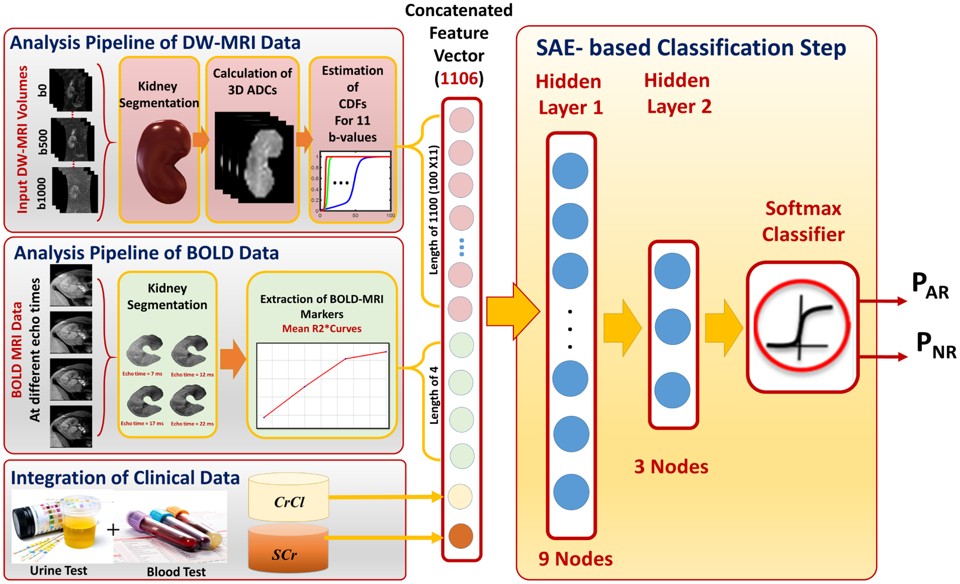
The proposed Renal-CAD system for early diagnosis of acute renal transplant rejection (AR). The input diffusion-weighted (DW) and blood oxygen level-dependent (BOLD) MRI data acquired at 11-different b-values and 5-different echo-times are first segmented. Then, the DW-MR image markers (cumulative distribution function (CDF) of the voxel-wise apparent diffusion coefficients (ADCs)) and the BOLD-MR image markers (mean R2* curve) are constructed. These image markers are then integrated with clinical biomarkers (creatinine clearance (CrCl) and serum creatinine (SCr)) and are fed into a stacked autoencoder (SAE) with a softmax classifier to obtain the final diagnosis as AR or non-rejection (NR).

II. MATERIALS

Forty seven patients who underwent renal transplantation were enrolled in this study after providing consent. DW-MRI scans (n = 47 patients), BOLD-MRI scans (n = 30 patients), and renal biopsies (n = 47, M = 31, F = 16, age = 35 ± 16.13 years, age range = 12–65 years) were obtained (June 2016 to June 2019) from two geographically diverse countries (USA and Egypt). For the DW-MRI and biopsy data, two groups were identified: NR group (30 patients) and AR group (17 patients). BOLD-MRI data included 20 NR patients and 10 AR patients. Kidney function for all patients participating in this study, as a part of post-transplantation routine medical care, were assessed with their laboratory values, namely; creatinine clearance (CrCl) and serum creatinine (SCr). The NR group (30 patients) had an average SCr value of 1.20 ± 0.36 mg/dl and CrCl value of 74.83 ± 26.26 ml/min. The AR group (17 patients) had a mean SCr value of 1.63 ± 0.57 mg/dl and CrCl value of 54.05 ± 22.28 ml/min. Renal biopsies and coronal MRI data were acquired within 48 hours of each other. The biopsy results were used as the ground truth for comparison with the classification algorithm.

The 47 DW-MRI scans (30 in Egypt and 17 in the USA) were acquired using two similar 3T Ingenia MRI scanners (Philips Medical Systems, Best, The Netherlands) using a body coil and a gradient single-shot spin-echo echoplanar sequence. However, data acquisition protocols were different and are summarized in Table I. For both DW-MRI acquisition protocols, water signals were acquired at different b-values of b₀, b₅₀, and b₁₀₀–b₁₀₀₀ s/mm² at 100 increments, see Fig. 2.

TABLE I:

Summary of the DW-MRI acquisition protocols of the data collected in USA and Egypt. Note that TR/TE: repetition time/echo time, SZ: slice size, STH: slice thickness, IG: intersection gap, FOV: field of view, NCS: number of cross-sections.

	Acquisition Protocol Metric
	TR/TE	SZ (pixels)	STH (mm)	IG (mm)	FOV (cm)	NCS
Egypt (30)	4400/82	176×176	4	0	22	24
USA (17)	8000/93.7	256×256	4	0	36	38

FIG. 2:

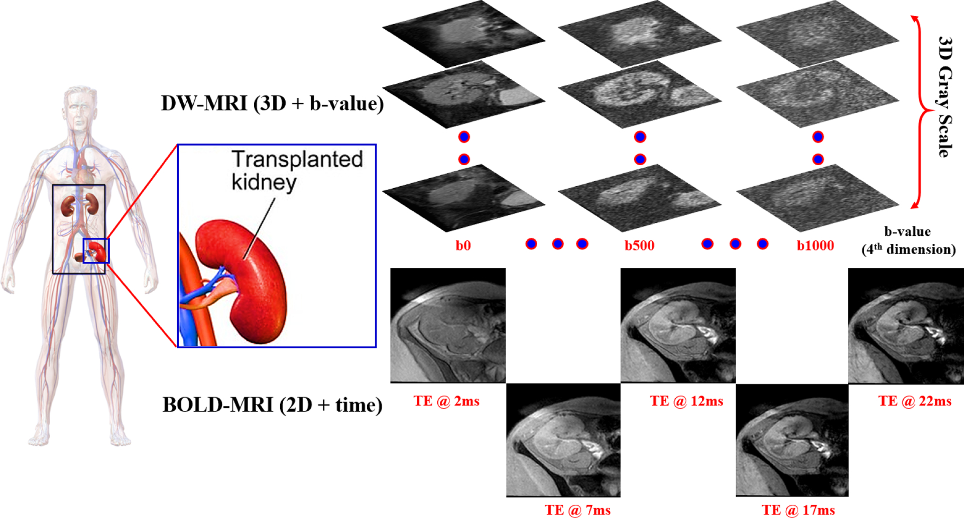
Data collection process demonstration for transplanted kidneys. DW-MRI data are collected at 11-different gradient field strengths and duration (b-values) of (b0, b50, b100, …, b1000 s/mm²), while BOLD-MRI data are collected at 5-different TEs (2, 7, 12, 17, 22 ms).

Thirty BOLD-MRI scans were acquired in Egypt using the same 3T scanner; TR: 140 ms, TE: 2 ms, Flip angle: 25°, Bandwidth: 150 kHz, slice size: 384 × 384, number of signals acquired: 1, FOV: 14.4 cm, thickness: 6.0 mm. For each subject, the middle/largest coronal image was selected and obtained at five different echo-times (TE = 2, 7, 12, 17, and 22 ms), see Fig. 2. Both biopsy reports and MRI scans were included in the final analysis and were examined by two clinicians, a radiologist and a nephrologist.

III. METHODS

An accurate Renal-CAD system, (see Fig. 1), to evaluate renal allograft status was developed. The Renal-CAD system applies the following steps to obtain the final diagnosis: (i) auto-segmentation of the renal allograft from surrounding tissues from DW- and BOLD-MR images; (ii) extraction of image markers; namely: cumulative distribution functions (CDFs) of the voxel-wise ADC maps and mean R2* values from the segmented kidneys using DW-MRI scans at different b-values and using BOLD-MRI scans at different echo-times acquired from two diverse geographical areas; (iii) integration of multimodal image markers with associated clinical biomarkers (SCr and CrCl); and (iv) diagnosing renal allograft status as NR or AR by utilizing these integrated biomarkers and our developed deep learning classification model built on stacked autoencoders (SAEs). Details of the developed Renal-CAD are discussed below.

A. Kidney Segmentation

Providing a fully-automated and precise segmentation of the renal allograft is a key step in the Renal-CAD system. Precise extraction of imaging features for accurate final diagnosis requires high segmentation accuracy. To improve segmentation accuracy, data preprocessing was performed prior to applying our previously developed segmentation approach²³, see Fig. 3. Briefly, histogram equalization was first applied on the bias corrected²⁴ MR images to suppress noise effects and image inconsistencies. Then, a nonrigid registration using B-splines approach²⁵ was employed to handle kidney motion and to reduce MRI anatomical variability among different patients to improve segmentation accuracy. Subsequently, renal segmentation based on the level-sets method²³ was performed. To enhance kidney segmentation accuracy, a joint Markov-Gibbs random field (MGRF) image model that combines three different components: shape, grey level, and spatial MRI features was employed. Renal segmentation approach accuracy was evaluated on all DW- and BOLD-MRIs for a more precise estimation of the discriminatory features. Two examples for our segmentation approach’s results for both DW- and BOLD-MRIs are shown in Figs. 4 and 5, respectively. Additional details of this approach has been described in Shehata et al.²³.

FIG. 3:

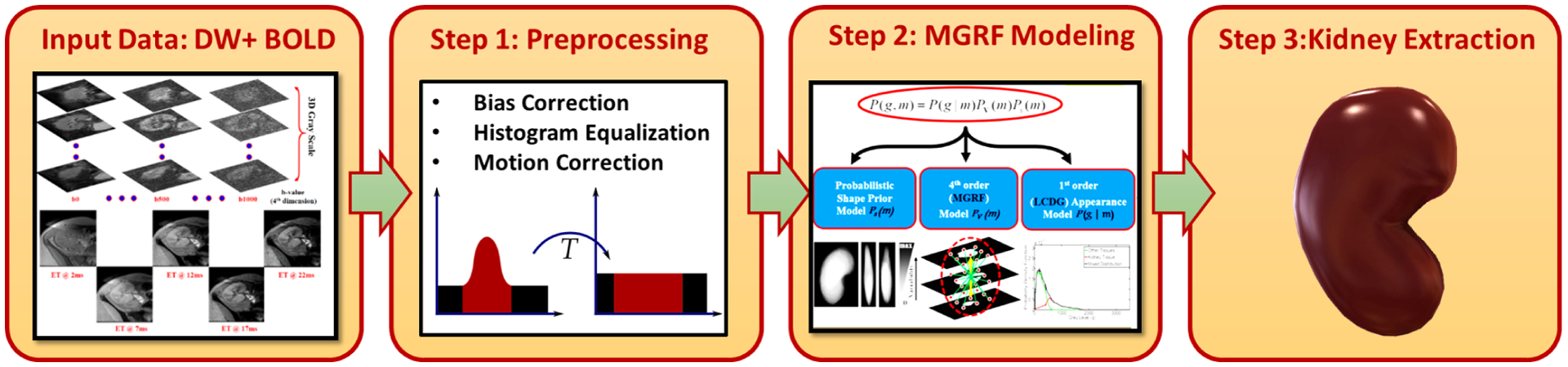
Block diagram illustrating the kidney segmentation approach’s steps²³. The raw DW- and BOLD-MRI data are first pre-processed to suppress noise and motion effects. Then, a joint Markov-Gibbs random field (MGRF) image model that accounts for the shape, intensity, and spatial features is employed. Finally, a level-set segmentation guided by the MGRF model is applied to get the final segmented kidney.

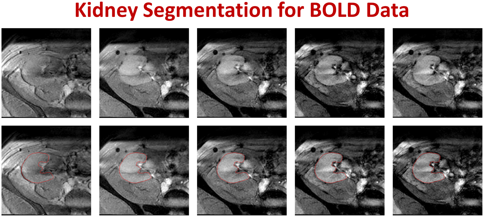
FIG. 4:

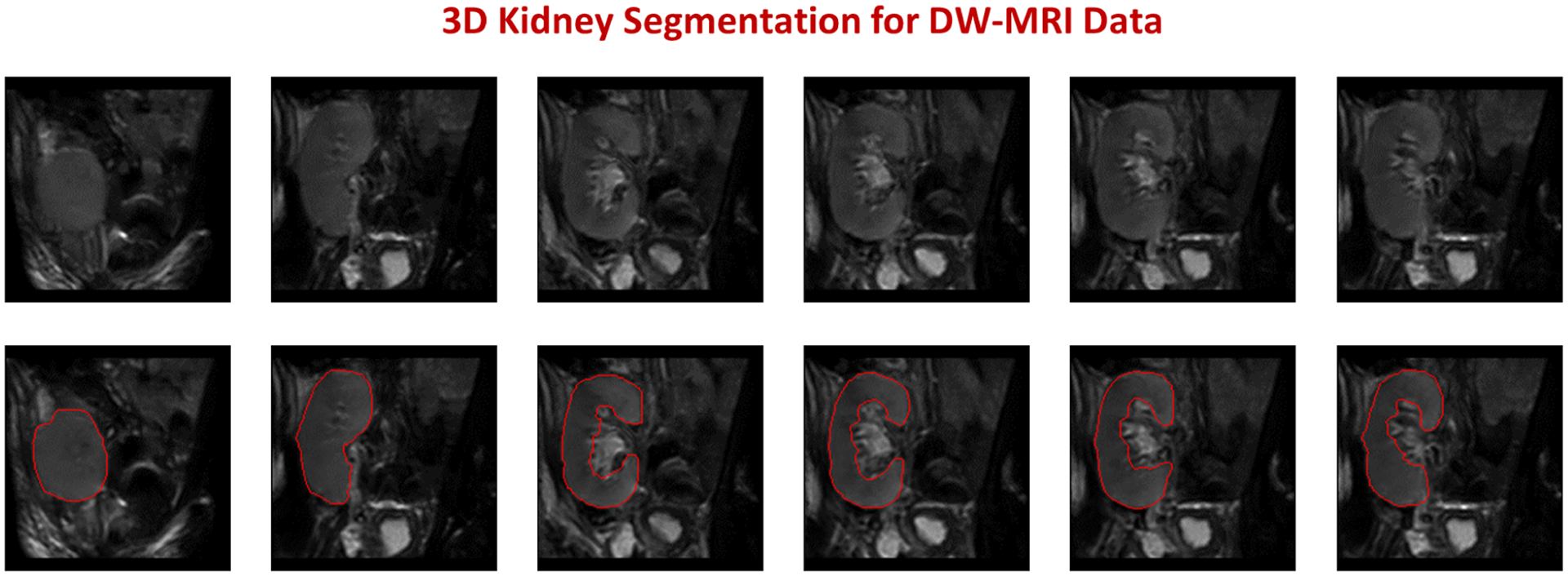
Segmentation results example for a DW-MRI subject. The upper raw shows different DW-MRI coronal cross-sections raw data, while the lower raw shows the corresponding segmentation results of our approach with red edges.

FIG. 5:

Segmentation results example for a BOLD-MRI subject. The upper raw shows different BOLD-MRI coronal cross-sections raw data at different echo times (from left to right: 2, 7, 12, 17, and 22 ms), while the lower raw shows the corresponding segmentation results of our approach with red edges.

B. Feature Extraction

1. Diffusion Weighted Imaging Markers:

The significant advantages of DW-MRI is highlighted by its ability to quantify local characteristics of blood diffusion and to interrelate them with the transplant status, due to DW-MRI’s ability to measure the unique characteristics of inner spatial water behavior in the soft tissue (e.g., kidney). This behavior is quantified by apparent diffusion coefficients (ADCs)^7,10,26, which can be utilized to evaluate the kidney transplant status. Following the accurate segmentation of the kidney, the DW-MR image-markers (i.e. voxel-wise ADCs) are estimated precisely using the following equation^27,28 as:

$${\text{ADC}}_{\text{vx}}=\frac{\text{ln}{g}_{0:\text{vx}}-\text{ln}{g}_{b:\text{vx}}}{b}$$ (1)

• vx: A voxel with its 3D Cartesian location (x, y, z).

• g₀: T2-weighted signal intensity obtained at b = 0.

• g_b: Diffusion-weighted signal intensity obtained at the given b-value.

The voxel-wise ADCs were estimated at the 11-different b-values to be used as discriminatory features to assess kidney transplant. However, using such voxel-wise ADCs as discriminatory features has the following limitations: (1) varying input data size that might lead to data truncation and/or zero padding for smaller and/or larger kidney volumes, respectively and (2) considerable training and classification time is needed, especially, in the case of large data volumes. In order to overcome these limitations, we characterized these voxel-wise ADCs at the 11-different b-values, using the cumulative distribution functions (CDFs) of the ADCs. To construct such CDFs, the minimum and maximum ADCs were calculated for all input datasets. Then, CDFs of the voxel-wise ADCs were constructed at the 11-different b-values (100 steps for each CDF) resulting in a DW-MR image markers (D_mrks) vector of size 1100 × 1. Please see Fig. 6

FIG. 6:

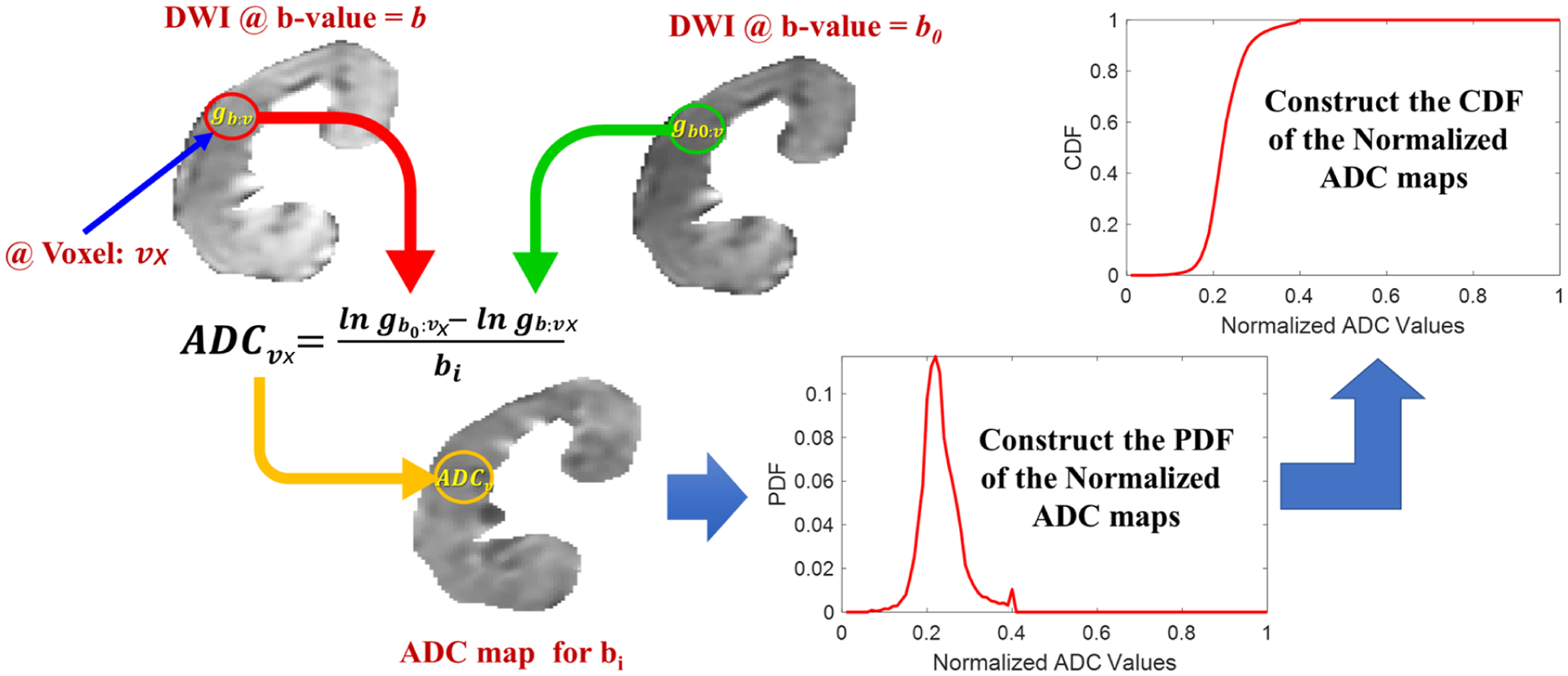
Demonstration of DW-MRI features construction procedure. First, the apparent diffusion coefficients (ADCs) are estimated from the segmented kidneys at 11-different b-values. Then, probability distribution functions (PDFs) and cumulative distribution functions (CDFs) are constructed consequently from the estimated ADCs at all b-values.

2. BOLD-MR Imaging Markers:

BOLD-MRI estimates the amount of the renal allograft content of deoxygenated hemoglobin (R2*). By measuring T2* (i.e., the amount of oxygenated hemoglobin¹⁹) in the allograft, one can calculate the R2* by taking the reciprocal of T2*. The mean R2* values were estimated from the delineated allograft using four different TE (7, 12, 17, 22 ms) resulting in a 4 × 1 vector of mean R2* values (Fig. 7). This vector was used as our discriminatory BOLD-MR image-markers (B_mrks) to assess renal allograft status. The BOLD-MRI data acquired at 2 ms was used as the baseline. The pixel-wise T2* and R2* maps can be estimated using the following equations¹⁸:

$$\text{T}{2}_{\text{px}}^{*}=\frac{t_0-t}{\text{ln}S{I}_{t:\text{px}}-\text{ln}S{I}_{t_0:\text{px}}}$$ (2)

$$\text{R}{2}_{\text{px}}^{*}=\frac{1}{\text{T}{2}_{\text{px}}^{*}}$$ (3)

FIG. 7:

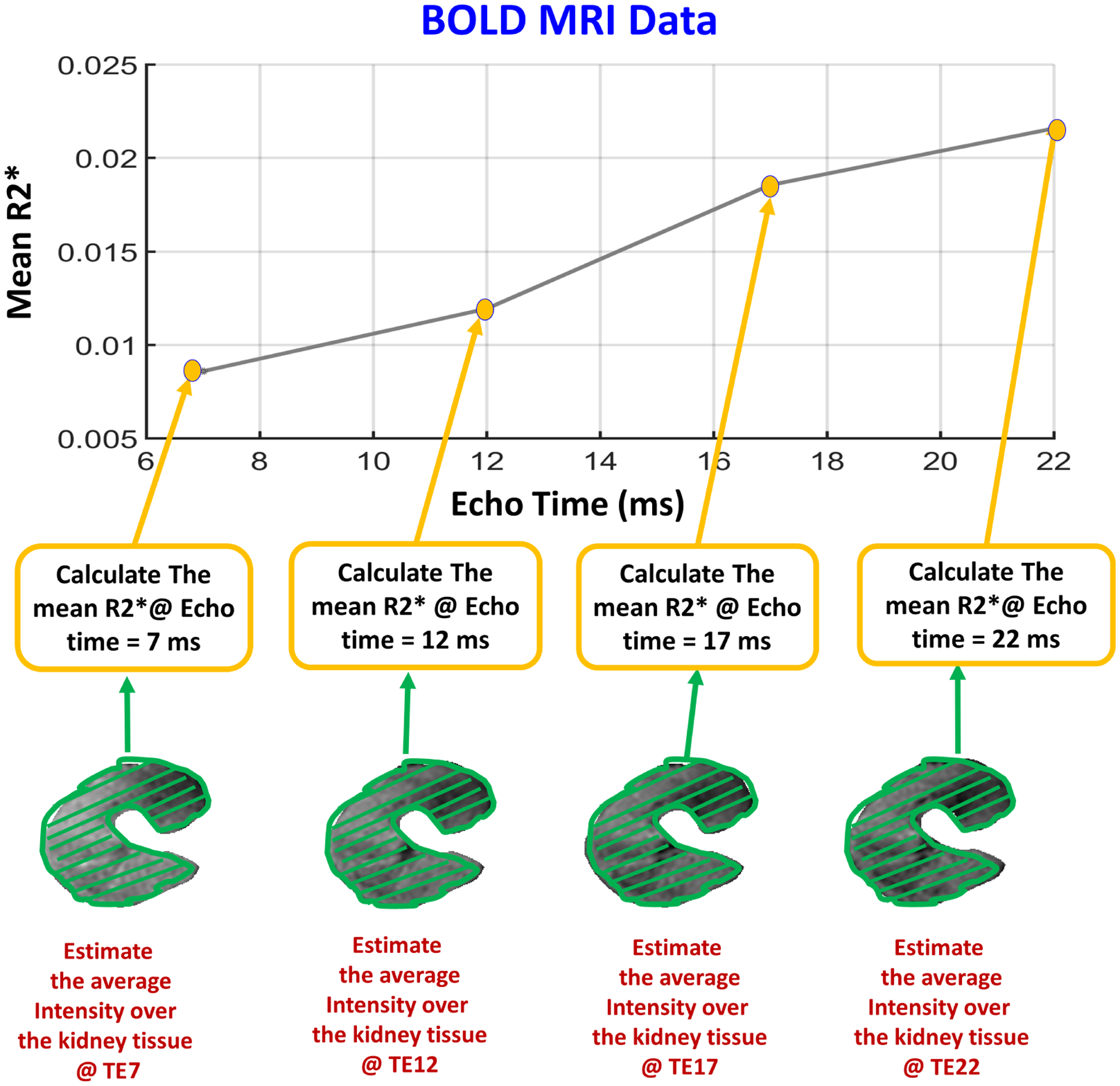
Demonstrating the procedure of constructing BOLD-MRI features, where the mean T2* values are estimated from the segmented allograft at 4-different echo-times (TE = 7, 12, 17, 22 ms). Then, the mean R2* values are estimated by taking the reciprocal of the estimated T2* values.

• px: a pixel with its 2D Cartesian location (x, y).

• SI_t: signal intensity obtained at TE = t and extracted from the segmented image.

• $S{I}_{t_0}$: signal intensity obtained at the baseline TE = 2 ms and extracted from the segmented image.

C. Deep Learning-based Stacked Autoencoders

Deep learning is a machine learning approach that is widely used in many applications, including in the medical domain (e.g., detection, diagnosis, prediction, etc.) for specific diseases. An autoencoder (AE) is an artificial neural network (ANN) that employs an unsupervised deep learning/training approach followed by a supervised backpropagation-based refinement algorithm to provide a better classification performance^29–31. The main structure of an AE, shown in Fig. 8, can be basically defined as three main types of layers: an input layer, a hidden layer, and an output layer. The AE training procedure can be classified into encoding and decoding processes. In the encoding process, the input data is mapped into a hidden representation through the hidden layer. In the decoding process, the input data are reconstructed from the hidden-layer representation. Both encoding and decoding processes are primarily used to learn an approximation to the identity function, which implies that the reconstructed input $\widehat{\text{X}}$ (i.e., decoding process output) is almost identical to the input X, see Fig. 8. The main purpose of this identity function is to force the AE to learn a compressed representation of the input, especially when the number of hidden nodes is less than the input size. Conversely, the AE is forced to reconstruct the input back given only the hidden features/activations.

FIG. 8:

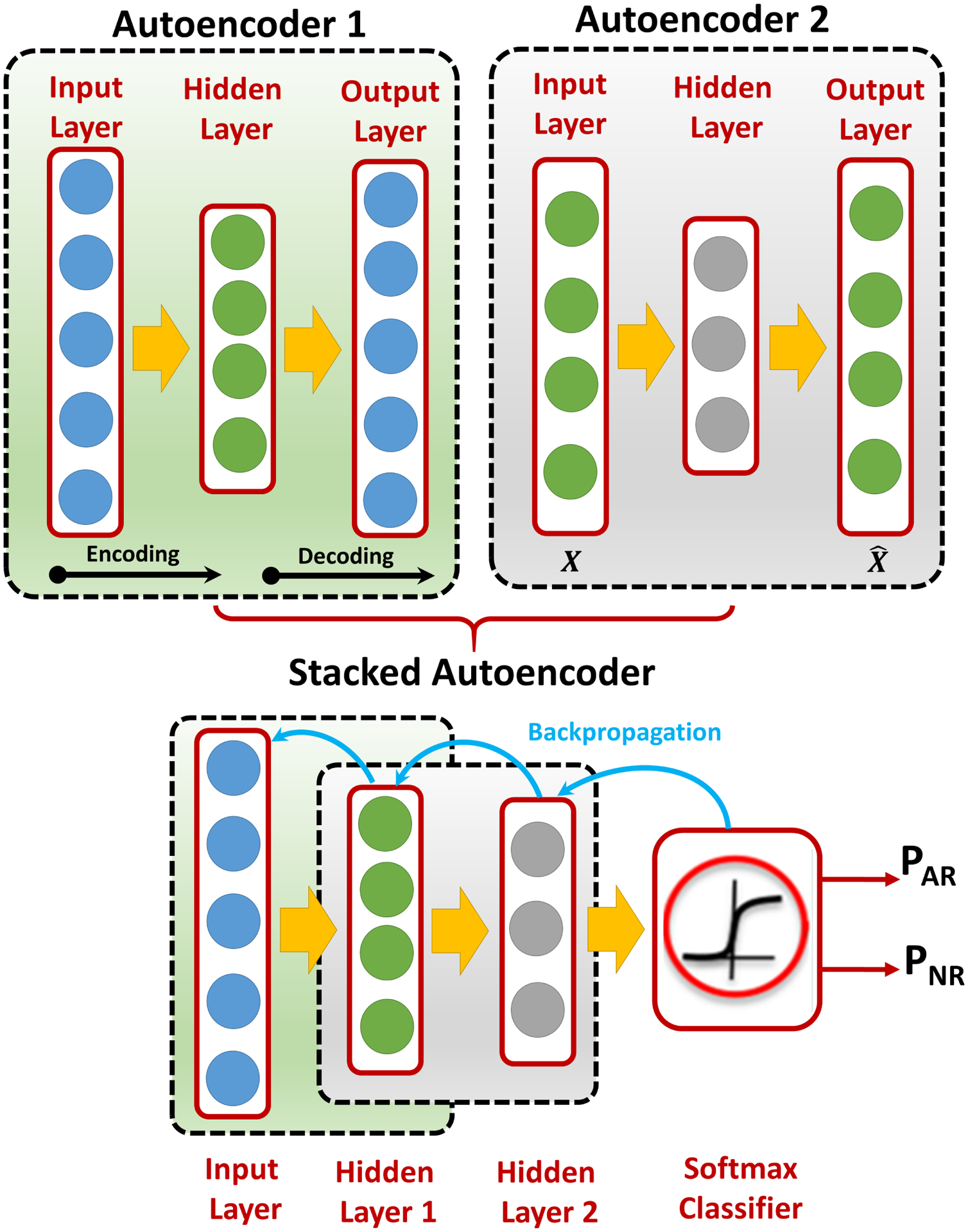
A demonstrative figure for the basic structure of the autoencoder (AE), where each AE consists of an input layer, a hidden layer, and an output layer. After training each AE separately, AE₁ is stacked with AE₂ and a softmax classifier on the top of them to obtain a stacked AE (SAE). Then, a backprobagation-refinement algorithm is used to update the hidden weights of the SAE.

Given the unlabeled training input dataset {X_n : n = 1 …N}, such that each ${\text{X}}_{\text{n}}\in {ℝ}^{\text{m}}$, ${\text{H}}_{\text{n}}\in {ℝ}^{\text{k}}$ represents the hidden layer’s features/activations resulting from the encoding process of the input vector X_n, this encoding process can be described by the following equation:

$${\text{H}}_{\text{n}}={\text{f}}_{\text{e}}\left({\text{W}}_{\text{e}}{\text{X}}_{\text{n}}+{\text{B}}_{\text{e}}\right),$$ (4)

where f_e represents the encoder activation function, which in this study is a sigmoid function, i.e. a differentiable, monotone scalar function with range (0, 1). ${\text{W}}_{\text{e}}\in {ℝ}^{\text{k}\times \text{m}}$ and ${\text{B}}_{\text{e}}\in {ℝ}^{\text{k}}$ are the weight matrix and the bias vector of the encoder, which are randomly initialized. Given the hidden layer’s features/activations H_n obtained from the aforementioned encoding process, the following equation describes the decoding process to obtain the reconstructed input $\widehat{\text{X}}$:

$${\widehat{\text{X}}}_{\text{n}}={\text{f}}_{\text{d}}\left({\text{W}}_{\text{d}}{\text{H}}_{\text{n}}+{\text{B}}_{\text{d}}\right),$$ (5)

where f_d represents the decoder function, while W_d and B_d are the weights and biases of the decoder, respectively. The optimal set of hyper-parameters of the AE can be tuned based on the compression/decompression reconstruction error minimization criteria as follows:

$$J_{\text{AE}}(\text{W},\text{B})=\frac{1}{2\text{n}}\sum _{i=1}^{\text{n}}{\Vert {\widehat{\text{X}}}_{\text{W}:i}-{\text{X}}_i\Vert }^2,$$ (6)

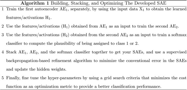
where ${\Vert {\widehat{\text{X}}}_{\text{W}:i}-{\text{X}}_i\Vert }^2$ represents the loss function that needs to be minimized, which in turn will lead to the reduction of the reconstruction error J_AE(W, B) at the end. To obtain our final stacked AEs (SAEs) that will be used in our Renal-CAD system for the early detection of AR, two autoencoders (AE₁ and AE₂) followed by a softmax classifier were trained and stacked together, see Fig. 9. Algorithm 1 summarizes building and optimizing our SAE.

FIG. 9:

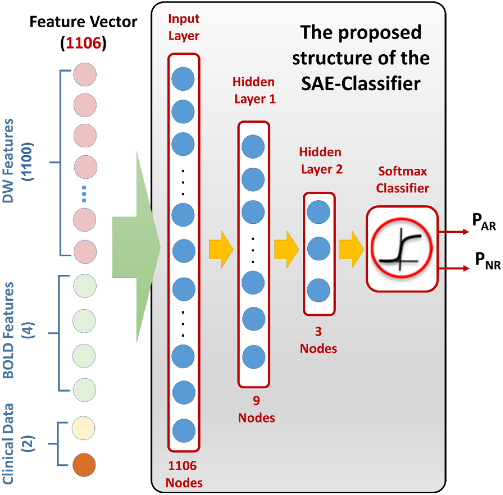
An illustrative figure showing the structure of the proposed SAE classifier. The feature vector uses the concatenation criteria to integrate diffusion markers with BOLD markers and clinical biomarkers. This vector is used as our SAE’s input and processed through two hidden layers and a softmax classifier to get the final probability of being an AR or NR renal allograft.

D. Overfitting and Dropout Technique

Deep neural networks (DNNs) are known with their complex structure, which makes them prone to overfitting. A DNN is overfitted when it fails to generalize or provide a correct analysis/output given a new set of input data. Overfitting typically occurs when the training set is not large enough. Dropout technique is a proven methodology for its ability to reduce overfitting in the training phase^32,33. Using dropout technique, one can obtain various representations for the relationships between the training data. Some of the hidden neurons can be randomly deactivated, while preserving their corresponding weights and biases, in each iteration during the training phase. In the next iteration, these deactivated neurons could be re-activated and some other different neurons might be deactivated. These permutating deactivation process leads to reduction in the total number of the activated neurons and thus hinder the complex co-adaptations between training data. In this manuscript, the dropout technique was used to suppress the overfitting effect by extracting meaningful features and to improve the final diagnostic accuracy of the developed Renal-CAD system.

E. Kidney Diagnosis by Integrating Diffusion, BOLD, and Clinical Biomarkers

To obtain an accurate assessment of the kidney transplant, we integrated the following different sources of information: (i) the estimated D_mrks vector of size 1100×1 to interrelate local blood diffusion characteristics with the transplant status; (ii) the estimated B_mrks vector of size 4×1 to quantify the amount of the renal allograft content of deoxygenated hemoglobin and interrelating it with the transplant status; and (iii) the combined clinical biomarkers (SCr and CrCl) resulting in C_bmrks vector of size 2×1 to measure the creatinine levels in both blood and urine, and thus; the filtration ability for renal transplant assessment. These three sources of information were integrated using the concatenation method resulting in an integrated biomarkers (I_bmrks) vector of size 1106×1 that will be used as our discriminatory features between the AR and NR groups.

After obtaining the I_bmrks, a classification process based on using a leave-one-subject-out cross-validation (LOSOCV) approach was employed using SAEs to obtain the final diagnosis. The I_bmrks of size 1106×1 were fed as an input vector to SAEs to build our classification model. A grid search algorithm minimizing the cost function as an optimization metric was employed to find the optimal-set of hyper-parameters. The two-layer SAEs with the first hidden layer (n = 9 nodes), second hidden layer (n = 3 nodes), output softmax layer (n = 2 nodes), weight decay parameter = 0.0022, weight of sparsity penalty term = 20, desired average activation of the hidden units = 0.2421, and dropout fraction = 0.5, provided the optimal diagnostic accuracy using LOSOCV approach and was selected for the proposed Renal-CAD system (Fig. 9).

IV. EXPERIMENTAL RESULTS

Two methods were used for train, test, and validation purposes. The first one is known as K-fold (i.e., LOSOCV) and is depending on training the network with all data while leaving only one subject outside for testing purpose. Then, in the next iteration, the network was reinitialized, and the subject that was left in the previous iteration was included back in the training data and the next subject was left outside for testing purpose. This procedure was repeated by the number of the subjects (N = 30, Training Data = 29, Testing Data = 1) and the diagnostic results were reported. The second validation is known as stratified 10-fold cross-validation in which 90% of the data were used for the training and 10% of the data were randomly selected and kept for testing. Then, in the next iteration, the network was reinitialized and that 10% was included back in the training set and another randomly selected 10% was kept for testing. This process was repeated for 10 times (N = 30, Training 255 Data = 27, Testing Data = 3).

It is worth mentioning that stratification was assured in the 10-fold cross-validation to help reduce both bias and variance. Stratification technique does not only allow for randomization but also ensures that the training/testing spilt percentages of each class in the entire data will be similar within each individual fold. In our case, NR = 20 subjects (67%) and AR = 10 subjects (33%), stratification ensures that 67% of our training data will be derived from NR subjects and 33% will be derived from AR subjects and the same percentages will be maintained for the test data too.

Renal-CAD software is primarily implemented in Matlab (The MathWorks, Natick, Mas-sachusetts), with time-critical subroutines developed in C using the Matlab Mex API. Cross-validation experiments were performed on a Dell Precision workstation with Intel Xeon eight-core CPU running at 2.1 GHz and 256 GiB RAM.

The developed Renal-CAD system with SAEs classifier was tested using the I_bmrks constructed for the 30 datasets that had both DW- and BOLD-MRI scans based on the LOSOCV approach. To demonstrate the effect of integrating D_mrks with B_mrks and C_bmrks and highlight its advantages, six additional scenarios were performed and compared with the Renal-CAD system using accuracy, sensitivity, and specificity as performance evaluation metrices, see Table II. The first scenario (S₁) utilized the D_mrks alone on the 47 datasets along with the same SAEs classifier and the LOSOCV approach. The second scenario (S₂) employed the B_mrks alone on the 30 datasets along with the same LOSOCV approach. However, because the B_mrks are of smaller size (i.e. 4×30), SAEs were replaced with a conventional multi-layer preceptron artificial neural network (MLP-ANN) classifier with two hidden layers (hl₁, n = 3 nodes and hl₂, n = 1 node). The third scenario (S₃) used the C_bmrks alone on the 47 datasets along with the same LOSOCV approach. However, because the C_bmrks are of smaller size (i.e. 2×47), the SAEs were replaced by a linear discriminant analysis (LDA) classifier. The fourth scenario (S₄) integrated both D_mrks with B_mrks resulting in DB_mrks on the 30 datasets along with the same SAEs classifier and the LOSOCV approach. The fifth scenario (S₅) integrated both D_mrks with C_mrks resulting in DC_mrks on the 47 datasets along with the same SAEs classifier and the LOSOCV approach. The sixth scenario (S₆) integrated both B_mrks with C_mrks resulting in BC_mrks on the 30 datasets along with the same LOSOCV approach. However, because the BC_mrks are of smaller size (i.e. 6×30), SAEs were replaced with a MLP-ANN classifier with two hidden layers (hl₁, n = 5 nodes and hl₂, n = 1 node). Results in Table II suggests that the utilization of the I_bmrks had a positive effect on the final diagnostic accuracy. This can be justified in part by the different abilities of each individual marker (i.e. D_mrks, B_mrks, and C_bmrks) to evaluate renal allograft function, which are complementary to each other.

TABLE II:

Diagnostic performance comparison between the proposed Renal-CAD system using the integrated biomarkers (I_bmrks) and six other scenarios S₁, S₂, S₃, S₄, S₅, and S₆ using the individual DW-MR image markers (D_mrks), BOLD-MR image markers (B_mrks), clinical biomarkers (C_bmrks), integrated diffusion and BOLD markers DB_mrks, integrated diffusion and clinical biomarkers DC_mrks, and integrated BOLD and clinical biomarkers BC_mrks respectively. Let Acc: accuracy, Sens: sensitivity, Spec: specificity, and AUC: area under the curve.

	Classification Performance (NR vs. AR)
	S1(Dmrks)	S2(Bmrks)	S3(Cbmrks)	S4(DBmrks)	S5(DCmrks)	S6(BCmrks)	Renal-CAD(Imrks)
Acc%	80.9	86.7	70.2	90.0	87.2	90.0	93.3
Sens%	76.5	80.0	80.0	90.0	82.4	80.0	90.0
Spec%	83.3	90.0	52.9	90.0	90.0	95.0	95.0
AUC	0.84	0.84	0.71	0.90	0.88	0.88	0.92

To ensure that the developed Renal-CAD system is not prone to overfitting (i.e., after using the dropout technique) and to validate the reproducibility and robustness of the Renal-CAD system, we performed a stratified 10-fold cross-validation approach on the same dataset (N = 30) using the same integrated biomarkers I_bmrks and the same SAEs with its previously defined structure and hyper-parameters. Results are reported in Table III and compared with the results obtained earlier using the LOSOCV approach in terms of accuracy, sensitivity, specificity, and area under the curve (AUC). In addition, the LOSOCV experiment was repeated 100 times with different randomly selected network initialization to ensure that the Renal-CAD system would be able to produce consistent diagnostic results. The Renal-CAD system produced the following diagnostic results: 91.65 ± 1.74 (% accuracy), 90.0 ± 0.0 (% sensitivity), and 92.5±2.64 (% specificity). These validation experiments demonstrated the reproducibility and robustness of the Renal-CAD system.

TABLE III:

Diagnostic performance of the developed Renal-CAD system using the integrated biomarkers (I_bmrks) using LOSOCV approach vs. 10-fold cross-validation approach. Let Acc: accuracy, Sens: sensitivity, Spec: specificity, and AUC: area under the curve.

	Classification Performance (NR vs. AR)
	Acc%	Sens%	Spec%	AUC
Renal-CAD (LOSOCV)	93.3	90.0	95.0	92.0
Renal-CAD (10-fold)	86.7	80.0	90.0	0.88

Statistical analysis was performed using R version 3.6. Differences in ADC or R2* between groups (AR/NR) were analyzed using MANOVA. Statistical significance was estimated from Pillai’s trace, converted into its approximately equivalent F statistic. MANOVA was performed using the individual imaging parameters by themselves, combined imaging parameters, and also in combination with lab values (CrCl and SCr). Follow up comparisons of ADC or R2* at each individual b-value or time point, respectively, were made using t-tests.

From Tables IV and V, renal allografts without AR had a slightly higher, albeit not significantly, mean ADCs at individual b-values, particularly with higher gradients ≥ 200, compared to AR. When all gradients were combined together, NR group had significantly higher ADCs than the AR group. The AR renal allografts had a higher, but not significant, mean R2* at the different echo-times (i.e. lower T2* values, which means lower amount of oxygen supply). Similarly, the combined R2* model did not reach significant differences. Table VI demonstrates the statistical significance between the two groups (AR vs. NR) using the individual clinical biomarkers, all of the possible pair-wise multivariate combinations, and the combination of the imaging modalities with the clinical biomarkers (All). As reported in Table VI, the CrCl and SCr have shown statistically significant differences between the two groups (the NR group demonstrated higher CrCl values and lower SCr values than the AR group). In addition, all possible pair-wise combinations and the combined model (All) demonstrated statistical significance between the two groups.

TABLE IV:

A comparison in terms of means and standard deviations (stds) of the ADC maps at 11-individual b-values between the non-rejection (NR) group and the acute rejection (AR) group. Statistic is t with approximately 31 effective degrees of freedom in univariate case, F with 11 degrees of freedom in the numerator and 35 in the denominator in the multivariate case.

ADC Maps at Individual b-values: mean(std) ≈
b (s/mm2)	50	100	200	b300	400	500	600	700	800	900	1000	Combined
NR(30)	4.0(0.66)	3.31(0.48)	2.86(0.31)	2.62(0.25)	2.48(0.20)	2.35(0.18)	2.25(0.15)	2.17(0.13)	2.09(0.12)	2.01(0.12)	1.94(0.11)	– – – – –
AR(17)	3.99(0.71)	3.37(0.48)	2.81(0.36)	2.53(0.32)	2.37(0.25)	2.26(0.23)	2.17(0.23)	2.07(0.22)	2.00(0.20)	1.93(0.19)	1.87(0.18)	– – – – –
Statistics	−0.016	0.368	−0.465	−1.00	−1.52	−1.40	−1.36	−1.62	−1.65	−1.61	−1.56	2.49
p-value	0.987	0.715	0.645	0.326	0.139	0.173	0.188	0.119	0.113	0.120	0.133	0.020

TABLE V:

A comparison in terms of means and standard deviations (std) of the R2* maps at 4-individual echo-times between the non-rejection (NR) group and the acute rejection (AR) group. Statistic is t with approximately 13 effective degrees of freedom in univariate case, F with 4 degrees of freedom in the numerator and 25 in the denominator in the multivariate case.

R2*/s Values at Individual Echo-times: mean(std) ≈
Echo-time	7 ms	12 ms	17 ms	22 ms	Combined
NR(20)	23.6(18.0)	19.9(5.8)	19.9(7.2)	19.4(4.7)	– – – – –
AR(10)	25.1(16.8)	20.3(9.3)	23.7(11.3)	23.3(10.3)	– – – – –
Statistics	0.244	0.149	0.974	1.14	1.95
p-value	0.810	0.884	0.348	0.277	0.133

TABLE VI:

A comparison in terms of means and standard deviations (stds) of the clinical biomarkers (CrCl and SCr) between the non-rejection (NR) group and the acute rejection (AR) group.

Data	CrCl	SCr	Dmrks+Cmrks	Bmrks+Cmrks	Dmrks+Bmrks	All
NR	74.8(26.3)	1.2(0.4)	– – – –	– – – –	– – – – –	– – – – –
AR	54.1(22.3)	1.63(0.6)	– – – –	– – – –	– – – – –	– – – – –
Statistics	−2.88	2.81	2.51	3.78	3.00	3.57
d.f.	38.1	23.4	13/33	6/23	15/14	17/12
p-value	0.007	0.010	0.016	0.009	0.023	0.015

Note: d.f. denotes degree of freedom with different values depending on the combined variables.

The performance of the developed Renal-CAD system was evaluated by constructing the receiver operating characteristics (ROC)³⁴, see Fig. 10. Furthermore, the performance of Renal-CAD system was compared to the six scenarios (S₁, S₂, S₃, S₄, S₅, and S₆) in terms of area under the curve (AUC). The Renal-CAD demonstrated the highest AUC of 0.92, as shown in Table II and Fig. 10. In addition, reproducibility and robustness of the Renal-CAD system was confirmed by comparing the performance of the Renal-CAD using a 10-fold cross-validation to the LOSOCV approach in terms of ROC (Fig. 11) and AUC (Table III).

FIG. 10:

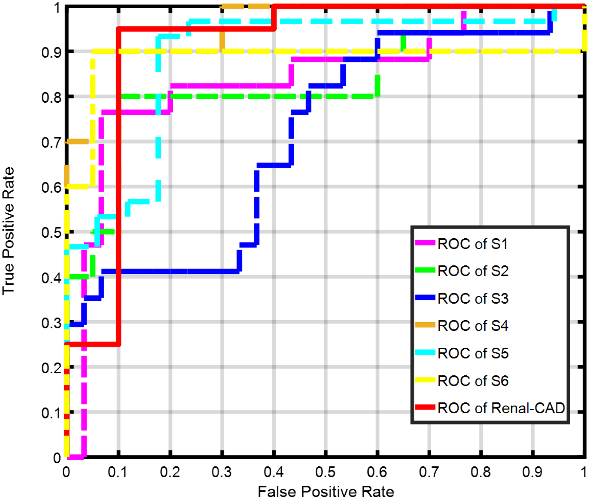
Receiver operating characteristics (ROC) curve for the proposed Renal-CAD system vs. six other different scenarios, namely; S₁, S₂, S₃, S₄, S₅, and S₆ using the individual DW-MR image markers (D_mrks), BOLD-MR image markers (B_mrks), clinical biomarkers (C_bmrks), the combined DW- and BOLD-MR image markers (DB_mrks), the combined DW-MR image markers and clinical biomarkers (DC_mrks), and the combined BOLD-MR image markers and clinical biomarkers (BC_mrks), respectively. The Renal-CAD area under the curve (AUC) is almost approaching the unity, demonstrating the feasibility and robustness of the developed system.

FIG. 11:

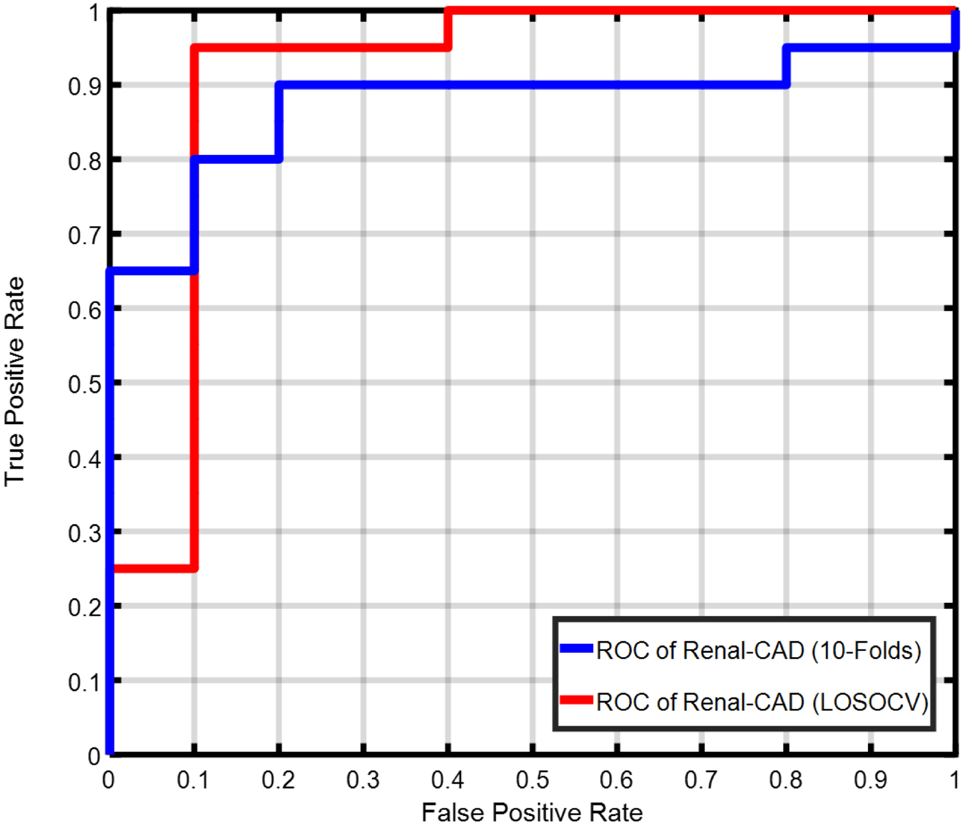
Receiver operating characteristics (ROC) curve for the proposed Renal-CAD system using the leave-one-subject-out cross-validation (LOSOCV) approach with an area under the curve (AUC) of 0.92 vs. using the 10-fold cross-validation approach with an AUC of 0.88. A reduction of only 0.04 in the AUC demonstrates the reproduciblity and robustness of the developed system.

V. DISCUSSION

The classification results of the Renal-CAD system that integrated multi-modal imaging markers and clinical biomarkers demonstrated high accuracy, sensitivity, and specificity. These results demonstrated the feasibility and efficacy of the Renal-CAD system to precisely and non-invasively identify renal allograft status at an early stage. Classification results obtained using individual imaging modalities (DW-MRI or BOLD-MRI) had lower accuracy, sensitivity, specificity, and area under the curve compared to the Renal-CAD system. The estimated diffusion markers (D_mrks) has the potential to interrelate local blood perfusion and water diffusion characteristics with the transplant status and thus, provide a good discriminator between AR and NR renal transplants. Most of the clinical studies estimated the ADC values at two selected b-values. Usually, they select one with a low gradient strength b-values < 200 to be able to measure blood perfusion^35,36 and one with a high gradient strength > 200 to be able to measure water diffusion inside the kidney^35–38. This study utilized 11-different gradients to estimate both blood perfusion and water diffusion to enhance diagnostic accuracy. The obtained results are in line with the findings of other clinical studies^{6,8–11,21,39–41} in that the NR renal transplants demonstrated higher ADC values than AR transplants (b-value > 200).

The estimated BOLD-MRI markers (B_mrks) can quantify the amount of the renal allograft content of deoxygenated hemoglobin to interrelate with the transplant status. There is no consensus regarding whether NR or AR has higher R2* values. Further, the threshold R2* values to distinguish AR from NR are not known^13,14,19. The findings of this study suggest that AR renal allografts demonstrate higher values of R2* at the different echo-times as previously reported^12,22. This can be physiologically justified in part by the fact that the change in oxygenation in the medulla may be associated with an almost hypoxic condition that makes it vulnerable to a further decrease in oxygen supply.

Clinicians are able to measure the creatinine levels in both blood and urine, and thus; the filtration ability for renal transplant assessment. However, these clinical biomarkers are imprecise and usually a later stage indication of rejection, when the damage to the kidney and the loss of renal function can be substantial. The developed Renal-CAD system integrates all available information to enhance diagnostic accuracy (93.3%), sensitivity (90.0%), specificity (95.0%), and AUC (0.92). This improved diagnostic ability is due to the integration of each individual marker (i.e. D_mrks, B_mrks, and C_bmrks) that can capture different aspects of renal allograft dysfunction that are complementary. The Renal-CAD system is robust to handle missing data, while still providing reasonable accuracy, as evidenced by Table II.

This work has some limitations that should be taken into consideration including: (i) small number of subjects that had both types of scans (i.e. DW- and BOLD-MRI); (ii) only the DW-MRI analysis pipeline included data from different geographical areas; (iii) age and gender had not been included in this analysis; (iv) this study only explored the ability of determining whether the renal allograft can be classified as AR or NR but cannot fully identify different types of renal dysfunction (e.g., ATN). Additional imaging and clinical biomarker data is currently being collected to enhance the ability of the Renal-CAD system to identify additional renal dysfunction conditions, to enhance its clinical utility. Despite these limitations, the Renal-CAD system demonstrated the feasibility of combining multiple types of markers for renal dysfunction to identify AR at an early stage.

VI. CONCLUSIONS

In conclusion, the developed Renal-CAD system demonstrated a high classification accuracy (93.3%), sensitivity (90.0%), specificity (95.0%), and AUC (0.92) for early stage diagnosis of AR post-transplantation. Renal-CAD integrates individual biomarkers (i.e. clinical biomarkers with DW-MR and BOLD-MR image markers) for a better characterization of renal allograft function and accurate identification of AR. The Renal-CAD system will be further optimized by training and validating on a larger patient cohort using both DW- and BOLD-MRI data. In addition, genomic markers and histopathology image markers can also be integrated into the Renal-CAD system to enhance AR diagnostic accuracy and identify subtypes of AR for clinical treatment.