

Abstract
Equivalent circulating density (ECD) is considered a critical parameter during the drilling operation, as it could lead to severe problems related to the well control such as fracturing the drilled formation and circulation loss. The conventional way to determine the ECD is either by carrying out the downhole tool measurements or by using mathematical models. The downhole measurement is costly and has some limitations with the practical operations, while the mathematical models do not provide a high level of accuracy. Determination of the ECD should have a high level of accuracy, and therefore, the objective of this study is to employ machine learning techniques such as artificial neural networks (ANNs) and adaptive network-based fuzzy inference systems (ANFISs) to predict the ECD from only the drilling data with a high accuracy level. The study utilized drilling data from a horizontal drilling section that includes drilling parameters (penetration rate, rotating speed, torque, weight on bit, pumping rate, and pressure of standpipe). The models were built and tested from a data set that has 3570 data points, and another data set of 1130 measurements was employed for validating the models. The accuracy of the models was determined by key performance indices, which are the coefficient of correlation (R) and the average absolute percentage error (AAPE). The results showed the strong prediction capability for ECD from the two models through training, testing, and validation processes with R greater than 0.98 and a very low error of 0.3% for the ANN model, while ANFIS recorded R of 0.96 and AAPE of 0.7, and hence, the two models showed great performance for ECD estimation application. Also, the study introduces a newly developed equation for ECD determination from drilling data in real time.
Introduction
Equivalent circulating density (ECD) is an important parameter for monitoring the drilling operations, especially for the narrow window between the formation and the fracture pressure. ECD is the total pressure of the mud hydrostatic column and the annular losses, and hence, it shows the mud pressure against the formation in the case of mud circulation.1 Therefore, it is critical to estimate the ECD with a high degree of precision to avoid any well control problems such as fracturing the drilled formation and circulation loss.
During the drilling operations, several factors were found to have an impact on the ECD, and among them were the annular pressure losses, wellbore geometry, mud properties (density and viscosity), mud pumping rate, downhole pressure and temperature, and concentration of cuttings.2−5
ECD can be acquired by means of downhole measurements, estimation using mathematical models, and/or predicting with the help of artificial intelligence (AI) techniques. A new technology in drilling tools helps implement a continuous circulating tool to monitor the ECD and provide good control for the formation pressure.6 Downhole measurements of the ECD are carried out using downhole sensors and pressure while drilling.7,8 The downhole measurement is considered accurate and robust for ECD values; however, the implementation of these downhole tools is not common due to the expensive daily charge and operational limitations such as downhole pressure and temperature that cause the tool failures.
Several mathematical correlations exist in the literature for estimating the ECD that are different in the fluid type and the parameters utilized as inputs. ECD estimation by implementing the material balance calculation for the mud compositional analysis was studied.9 However, the models had many assumptions and limitations regarding the downhole pressure, temperature, and mud types. Bybee10 introduced a mathematical equation to calculate the ECD. The model considers the effect of concentration of solids on the annular losses, in addition to the mud static density and other mud-related parameters.
The developed mathematical correlations are limited to some applications, and they ignore a lot of other input parameters that have an impact on the ECD values. Such ignored parameters are well geometry, fluid rheological properties, rotation of the drill string, and downhole pressure and temperature conditions, which affect the mud density, cuttings dispersion, hole cleaning, and swab and surge of drill pipe movements in the hole.11,12 Ignoring these parameters will affect the ECD prediction, lead to inaccurate evaluation of ECD, and cause well control problems during the drilling operations.13,14
Predicting ECD by Employing ML Techniques
ECD prediction from the drilling data is considered a novel approach in the petroleum industry due to the limitations of the ECD downhole measurements. AI is a technique that utilizes high computing capabilities for processing advanced algorithms to solve technical/problematic issues by simulating the human brain’s thinking manner.15 ML has many tools like artificial neural networks (ANNs), adaptive neuro-fuzzy inference systems (ANFISs), support vector machine (SVM), and functional networks (FNs) that show high performance and accuracy level for prediction and classification problems.16 The implementation of ML has wide applications in many disciplines of engineering, economics, medicine, military, marine sectors, and so forth.17,18 ANNs mimic the way the brain works; they forecast without knowing statistics and are computer programs that learn patterns. An ANFIS is a type of ANN that uses the Takagi–Sugeno FIS as its base and a set of fuzzy if-then rules. The ANFIS offers the ability to capture the benefits of both neural networks and fuzzy logic principles in a single framework because it integrates both. The FNs technique is a unique generalization of neural networks that combines domain knowledge, which is used to design the network’s topology, with data, which are used to estimate unknown neuron functions. It is worth mentioning that neural networks are special cases of FNs. SVM is a supervised learning approach for solving high-complexity regression and classification problems. SVM moves data from a lower-dimensional to a higher-dimensional space, known as kernel space, allowing for more training instances.
In the oil and gas industry, many studies utilized ML techniques for finding solutions for practical challenges.19−22 Intelligent models were accomplished by AI tools for many purposes such as identifying the formation lithology,23 predicting the formation and fracture pressures,24 estimating the properties of reservoir fluids,25 estimating the oil recovery factor,26,27 predicting the tops of the drilled formation,28 rate of penetration (ROP) prediction and optimization for different drilled formations and well profiles,29−31 determining the content of total organic carbon,32−34 and estimating the rock static Young’s modulus,35−38 predicting the compressional and shear sonic times,39 determining the rock failure parameters,40 detecting the downhole abnormalities during horizontal drilling,41 determining the wear of a drill bit from the drilling parameters,42 and predicting the rheological properties of drilling fluids in real time.31,43−46
For ECD prediction, Table 1 represents recent works that were performed for ECD prediction from the drilling and mud parameters. Ahmadi47 utilized the least square SVM (LLSVM), ANFIS, and enhanced particle swarm optimization PSO-ANFIS tools to estimate the ECD from only mud initial density, pressure, and temperature. The results showed the outperformance of ANN compared to the other tools. Ahmadi et al.48 predicted ECD by employing PSO-ANN, FIS, and a hybrid of genetic algorithm (GA) and FIS (GA-FIS) from the initial mud density, pressure, and temperature data. The PSO-ANN model presented a high degree of prediction performance in terms of coefficient of determination (R2) and average absolute percentage error between the actual and predicted values of ECD.
Table 1. ECD Prediction Models Using AI in the Literature.
| ref. | model | model inputs | data | R2 | AAPE |
|---|---|---|---|---|---|
| Ahmadi47 | LLSVM | pressure | not available | 0.9999 | 0.000145 |
| ANFIS | temperature | 0.8502 | 35.002 | ||
| PSO-ANFIS | initial density | 0.869 | |||
| Ahmadi et al.48 | PSO-ANN | pressure | 664 points from the literature | 0.9964 | 0.0001374 |
| FIS | temperature | 0.7273 | 67.0907 | ||
| GA-FIS | initial density | 0.9397 | 0.091 | ||
| Alkinani et al.49 | ANN | flow rate | 2000 wells | 0.982 | not available |
| mud weight | |||||
| plastic viscosity | |||||
| yield point | |||||
| TFA | |||||
| RPM | |||||
| WOB | |||||
| Abdelgawad et al.5 | ANFIS | mud weight | 2376 data points | 0.98 | 0.22 |
| ANN | drill pipe pressure | 8.5″ vertical hole section | |||
| rate of penetration | |||||
| Rahmati and Tatar50 | radial basis function | pressure | 884 points from the literature | 0.99 | MSE 0.00000166 |
| temperature | |||||
| type of mud | |||||
| initial density | |||||
| Alsaihati et al.51 | support vector machine, random forests, and functional network | flow rate | 3567 data points | 0.95–0.99 | RMSE From 0.23 to 0.42 |
| standpipe pressure | |||||
| hook load | |||||
| weight on bit | |||||
| torque | |||||
| rate of penetration | |||||
| drill string speed |
Alkinani et al.49 predicted the ECD using the ANN model that had only 1 hidden layer and 12 neurons, and the study utilized drilling parameters in addition to the hydraulics and mud properties such as mud pumping rate, properties of the mud (density, plastic viscosity, and yield point), total flow area (TFA) for the bite nozzles, revolutions per minute (RPM) for the drill pipe, and the weight on bit (WOB). Abdelgawad et al.5 provided a model for ECD prediction using two AI techniques, ANN and ANFIS. The study provided an ECD-ANN model of 1 hidden layer with 20 neurons, while the ANFIS model was developed by utilizing 5 membership functions, with the Gaussian membership function (gaussmf) as the input membership function and the output membership function being a linear type. Rahmati and Tatar50 employed radial basis function to build an ECD prediction model that showed good prediction capability with R2 of 0.98 and AAPE of 0.22. Recent work predicted the ECD while drilling horizontal sections using the surface drilling data by employing three different machine learning techniques.51 The study utilized SVM, random forests (RF), and FN to build the models using seven drilling parameters as inputs for the study, and the accuracy of the developed models ranged from R2 of 0.95–0.99 and root mean squared error (RMSE) ranged from 0.23 to 0.42. In this study, the author did not develop any ECD equation that can be used without the need for the machine learning code.
It is clear from the literature that the AI models enhanced the ECD prediction; however, the models are different in terms of the input parameters, the data used to feed the models, and the methodology followed for the ECD prediction. One of the shortcomings found from many studies in the literature is that the downhole pressure and temperature are required as inputs in the prediction models, and from an operational view, downhole sensors are required to obtain these parameters with high accuracy for better ECD prediction, and this will add operational cost and time for the data collecting. Consequently, the new contribution of this study is to employ available real-time drilling parameters from surface rig sensors to build ECD prediction models using ANN and ANFIS techniques.
The novel approach in this study is that the AI models are mainly dependent only on the mechanical drilling parameters such as mud pumping rate (GPM), ROP, drillstring speed in RPM, stand-pipe pressure (SPP), WOB, and drilling torque (T). Besides, the study presented an empirical correlation that can be easily utilized for ECD estimation from only the drilling parameters. The AI models that were presented in this study were validated from another data set to ensure high and robust performance for ECD prediction.
Materials and Methods
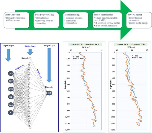
The study utilized real drilling data that were collected from the drilling operations from real-time sensors. Figure 1 presents, in brief, the processing flow to provide robust ECD models starting from data gathering, data cleaning, and filtering; to provide the model input parameters with good quality, the training process for the AI model, optimization of the model parameters with the trained algorithm, and accuracy testing for the model results are carried out, and if the accuracy is low, then re-training process is performed in order to get the optimum model parameters for high accuracy performance for the ECD prediction.
Figure 1.

Processing flow chart for ECD AI models.
Data Description
The data obtained for the current study were collected during a drilling phase in the Middle East. The data covered the horizontal section for drilling a 5–7/8-inch hole. A total of 3570 points was obtained after data preprocessing. The drilling parameters that were utilized as inputs for the model were collected from the surface rig sensors that represent GPM, ROP, RPM, SPP, WOB, and T. ECD data were collected from the downhole pressure tool and were used for the model output estimation. Also, another cleaned data set (1130 measurements) was employed for further model validation as an unseen data set to ensure the model prediction performance.
Data Cleaning and Statistical Analysis
The obtained data are preprocessed by using technical analysis for data cleaning. The collected data from the drilling sensors need special preprocessing in order to enhance the data quality. The data cleaning was performed by removing the missing and illogic values such as zero and negative values. In addition, the outliers have to be removed from the data, and this step was performed by using the box and whisker plot technique, in which the top whisker represents the upper limit of the data and the bottom whisker represents the lower limit of the data. The data quality has a great impact on the developed model performance.
Statistics, as an interdisciplinary field, plays a substantial role in both the theoretical and practical understanding of ML and for its future development. Statistical methods can be used in problem framing, data understanding, data cleaning, data selection, data preparation, model evaluation, model configuration, model selection, model presentation, and model predictions. The process of identifying and repairing issues with the data such as data loss, data corruption, and data errors is called data cleaning. Statistical methods are used to clean data using outlier detection and imputation. Not all observations or all variables may be relevant for modeling. The process of reducing the scope of data to those elements that are most important for prediction is called data selection. Two types of statistical methods that can be used for data selection: data sample and feature selection. Data may not be directly used for modeling; as a result, some transformations are required to change the shape or structure of the data to make them suitable for the selected problem frame or learning algorithm. Data preparation is conducted using some statistical methods including scaling such as standardization and normalization, encoding such as integer encoding, and transforms such as power transforms like the Box–Cox method. Model evaluation is a crucial part of predictive modeling and can be done by experimental design, which is a whole subfield of statistical methods. The interpretation and comparison of the results among various hyperparameter configurations are performed by one of two subfields of statistics, which are statistical hypothesis tests and estimation statistics. Finally, the model is used to predict new input data. At this stage, quantification of the prediction confidence via the field of estimation statistics is needed to quantify this uncertainty.
Figure 2 shows the correlation coefficients (R) between the output (ECD) and drilling parameters after preprocessing the data. The relative importance of the data showed that SPP and T have the highest R of 0.87 and 0.85, respectively, with the ECD, while the WOB showed the least R (−0.01) with the ECD, which indicates that the relationship might be a nonlinear type between ECD and WOB. It is noticed that T, SPP, and RPM showed a direct relationship with ECD, while GPM, ROP, and WOB presented an indirect relationship with ECD. Table 2 shows the statistical analysis for all parameters. The data showed the wide range of the parameters, as GPM ranged from 249.4 to 296.6 with 47.2 gallons per minute (gpm), ROP from 3.5 to 59.6 ft/h, SPP from 2379.7 to 3632.1 psi, RPM from 59 to 141.3, T from 3.7 to 10 kft Ib, and WOB from 5.5 to 20 kIb, and the ECD parameter has a range of 12.1 pounds per cubic feet (pcf) from a minimum value of 83.4 to a maximum value of 95.5 pcf. The maximum and minimum ranges show the data limits and whether the data cover a broad range or not. The standard deviation is the measure of dispersion, or how the data spread out around the mean in a data set. Using this metric to estimate the variability of a population or sample is an important test of a machine learning model’s accuracy against real-world data. Moreover, the standard deviation can be used to measure confidence in a model statistical conclusion. Skewness is a measure of how distorted the data are from the normal distribution. In most models, any form of skewness is undesirable, as it leads to an excessively large variance in estimations. Other models require unbiased estimators or Gaussian models to function accurately. In either case, the goal is to decrease skewness to reach as close as possible to a normal distribution by using transformations such as taking the inverse, logarithm, or square roots of all the datapoints. Kurtosis is a statistical measure used to describe the degree to which values cluster in the tail or the peak of a frequency distribution, often visually described by the sharpness of the peak values. Often, kurtosis values are compared with that of the normal distribution, as values less than 3 are said to be platykurtic or “flat-topped.” Alternatively, kurtosis values higher than 3 are said to be leptokurtic, usually appearing sharp at their peak values. The developed models are expected to have the same performance if the data set used falls in the same ranges of the data used for training the models. It is recommended to update the parameters of the models for other fields with different data ranges and geologic features to ensure a viable prediction with reasonable accuracy.
Figure 2.
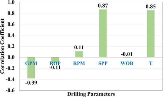
Correlation coefficients between the inputs and ECD after data preprocessing.
Table 2. Statistical Analysis for the Models Data.
| statistical parameter | GPM | ROP (ft/h) | RPM | SPP, psi | WOB (klb) | T (kft Ib) | ECD, pcf |
|---|---|---|---|---|---|---|---|
| minimum | 249.4 | 3.5 | 59.0 | 2379.7 | 5.5 | 3.7 | 83.4 |
| maximum | 296.6 | 59.6 | 141.3 | 3632.1 | 20.0 | 10.0 | 95.5 |
| range | 47.2 | 56.1 | 82.3 | 1252.4 | 14.6 | 6.3 | 12.1 |
| mean | 276.7 | 23.0 | 119.8 | 3035.3 | 15.2 | 6.9 | 90.4 |
| median | 281.0 | 23.7 | 120.0 | 3032.7 | 16.1 | 6.9 | 90.4 |
| standard deviation | 10.3 | 6.2 | 16.9 | 258.0 | 3.0 | 1.2 | 3.2 |
| Kurtosis | 1.11 | 1.88 | 1.28 | –0.14 | 0.08 | –0.87 | –0.89 |
| skewness | –1.67 | 0.22 | –0.93 | –0.15 | –0.96 | –0.05 | –0.39 |
Building AI Models
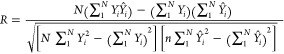
This study employed two techniques from the AI tools to develop ECD prediction models using only the drilling parameters. ANN and ANFIS techniques are trained using the input data using the training and testing ratio of 77:23. The training and testing data sets were randomly selected. The sensitivity analysis for each model parameter was carried out to determine the best model architecture. The model prediction was evaluated with two statistical parameters in addition to the ECD profiles for the actual and the predicted data. The correlation coefficient (R) and the average absolute percentage error (AAPE) were calculated by eqs 1 and 2.
| 1 |
 |
2 |
where N is the number of samples in the data set, Yi is the actual output, and Ŷi is the predicted output.
ANN Model
An ANN tool was utilized for solving engineering problems by its processing algorithms based on interconnected artificial neurons that mimic the biological neural networks.52,53 Three layers represented the common architecture for ANN, which are the input, hidden, and output layers.54 Weights and biases are utilized in the ANN structure to link the layers and affect the network performance.55 Different algorithms are used for the model training and controlling the neuron processing.56 Many parameters were tested to check its impact on the ANN model accuracy such as the hidden layer/s number, the neurons’ number, network, training, and transfer functions. The training/testing ratio was checked from a range of 70/30 up to 90/10. The hidden layers were from one to three layers. The number of neurons in the hidden layer was tested from 5 to 40. Several network functions such as fitnet, newfit, newcf, newelm, newlrn, newpr, newdtdnn, newff, newfftd, and newfit were tested, while training functions such as trainbr, trainoss, trainlm, trainbfg, and traingdx were checked for the best results. Sensitivity analysis was performed for the transfer functions such as tansig, satlin, purelin, softmax, and logsig, which were tried for the ANN structure. Figure 3 shows the design of the developed ANN model used in this study.
Figure 3.
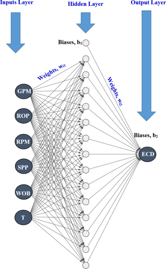
Architecture of the developed ANN model.
ANFIS Model
ANFIS was established in the early 1990s as a type of ANN that depends on the Takagi–Sugeno FIS.57 The interface of the ANFIS utilized a set of fuzzy “if-then rules” that can learn and optimize the nonlinear functions.58 ANFIS architecture consists of four layers. The first layer, called the fuzzification layer, collects the inputs and determines the membership functions (e.g., sigmoid, gaussian, trapezoidal, or straight line). The second layer, denoted as “rule layer,” applies many fuzzy “if-then” rules. In the third layer, databases are employed for membership function rules, and the decision-making unit is developed for the inference operations, while in the last layer, the defuzzification interface is used.58
The ANFIS model was developed using the subtractive clustering method. The cluster radius and number of iterations are ANFIS parameters that were checked for the optimization process. The sensitivity analysis for the model parameter is a key step in the model development and especially the cluster radius for the ANFIS tool.
Results and Discussion
This section discusses the results obtained from the two AI-developed models for predicting the ECD from the real-time drilling parameters.
ANN Results
The cleaned data that were used to feed the model algorithms for training purposes is plotted in terms of all the inputs/drilling parameters and the model output/ECD value to illustrate the data profiles along with the depth of interest for the study (Figure 4). The depth is presented in the form of depth index, which refers to the bit depth. The data profiles reveal the complexity of the relationship among the drilling parameters and between them and the ECD. The applications of AI helped more to reveal the complex relationship such as for the current scope of work.
Figure 4.

Data profiles for the inputs and output parameters.
The designed ANN code was optimized by testing many scenarios to achieve the best model parameters, which are listed in Table 3. For each code run, only one parameter option was tested, and the results were recorded. After running the specially designed MATLAB program, the authors compared the different kinds of errors and the correlation coefficient between the actual and predicted values, and the optimum combination of the hyperparameters was selected to qualify to the validation stage. Table 4 shows an example of the best results obtained out of several trial runs during the training and testing stages. The error decreased with the neurons increasing from 5 to 15, and then, the error increased again with the neurons increasing from 15 to 35. As a result, 15 neurons were selected to be fixed in the upcoming runs while changing the other hyperparameters. The authors found that using a few neurons may lead to bad results due to underfitting and using too many neurons may lead to overfitting issues. Network type was the second hyperparameter to be changed, and newfit was chosen, as it gave better results compared to the others. Training function was the third parameter to be changed, while keeping the other constant, and trainlm gave the optimum performance in terms of errors and R for training and testing. The transfer function was the fourth variable; hyperparameter and softmax transfer function provided the best performance compared to the others. After selecting the optimum hyperparameters within a single layer, the effect of the layer number in the neural network was tested. As the layers increased, the errors started to increase, and the R decreased. Therefore, it was decided to proceed with a single layer, as it will enhance the performance, and the model will be simpler regarding application and equations extraction as well. The increasing layer number may result in an overfitting issue, which leads to high accuracy for training data and low accuracy for testing data. By the end of the optimization process, the optimum combination of the model parameters was recognized. The training to testing ratio for the data sets was found to be 77:23—2743 data points for training and 827 points of data for the testing process. Only one hidden layer with 15 neurons was enough to achieve a better prediction accuracy. The best network, training, and transfer functions were fitting network (newfit), Levenberg–Marquardt backpropagation (trainlm), and softmax, respectively, and 0.12 is the optimum learning rate.
Table 3. Tested Options for ANN Parameters.
| model parameter | options | ||
|---|---|---|---|
| training/testing ratio | )70/30(−(90/10) | ||
| hidden layers | 1–4 | ||
| number of neurons | 5–40 | ||
| network function | fitnet | newfit | newcf |
| newelm | newlrn | newpr | |
| newdtdnn | newff | ||
| newfftd | newfit | ||
| training function | trainbr | trainoss | trainlm |
| trainbfg | traingdx | ||
| transfer function | tansig | satlin | purelin |
| logsig | netinv | softmax | |
| hardlims | radbas | tribas | |
| learning rate | 0.01–0.9 | ||
Table 4. Best Results for Training and Testing the ANN Model.
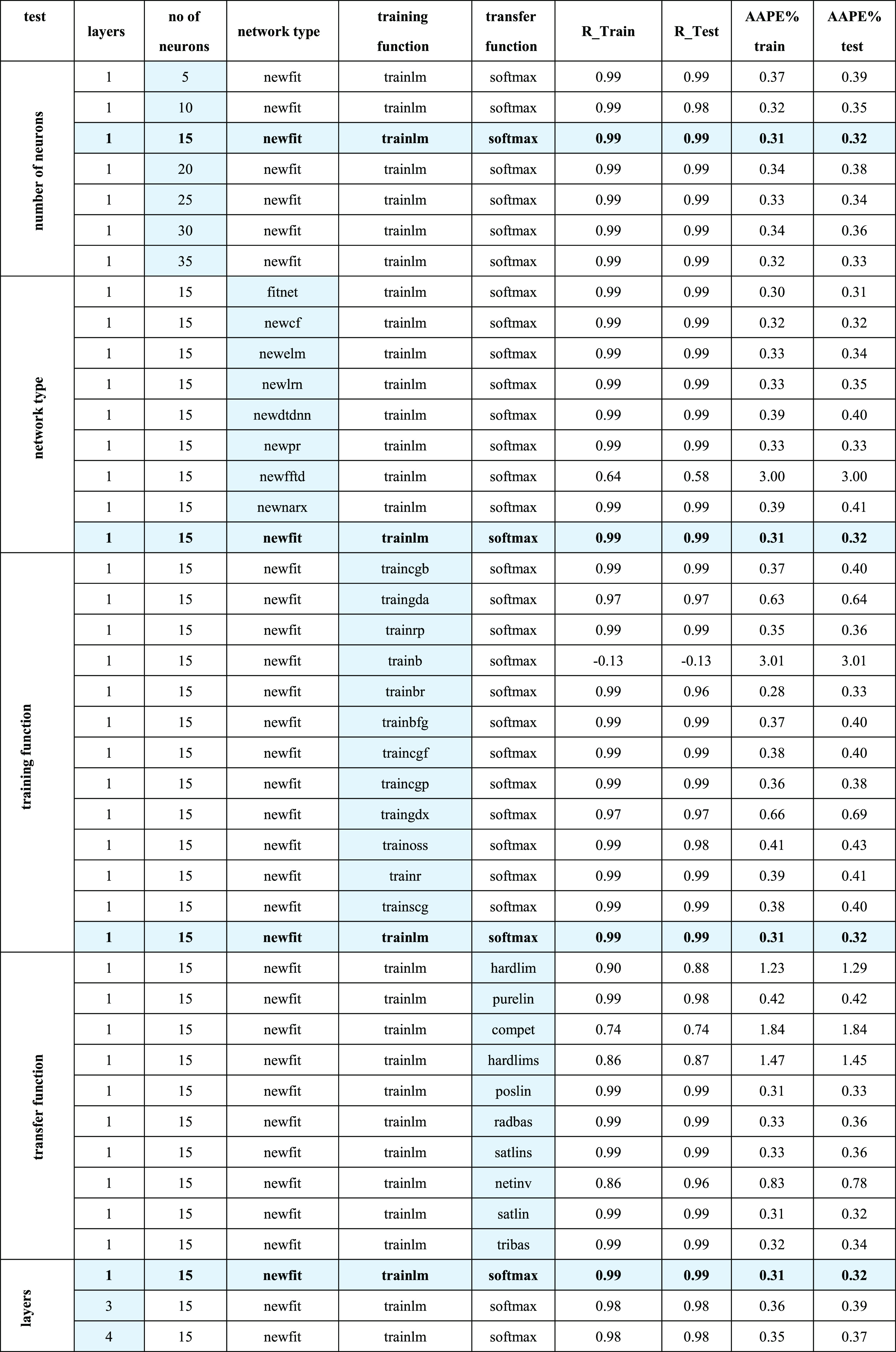
Figure 5 represents the cross-plots for the ANN results for the model training and testing processes for estimating ECD values. The results showed a strong accuracy for the model in terms of R and AAPE for both training and testing, as R was 0.99 between the real and predicted values for the ECD for training and testing, while the AAPE was 0.33 and 0.32 for training and testing, respectively. The plots reveal that there is no unaccepted over- or underestimation for the predicted value, which shows the high accuracy for the models’ prediction performance.
Figure 5.

Cross-plots between the predicted and actual ECD results from the developed ANN model. (a) Training process and (b) testing process.
ANFIS Results
The same procedures were followed for optimizing the model parameters; however, cluster radius and iterations number are the target parameters for the ANFIS model. After several runs for the ANFIS code, the optimum parameters were found as 0.8 for the cluster radius and 300 for the number of iterations. Figure 6 displays the ANFIS results for the model training and testing processes. In addition, there were similar accepted model predictions for ECD values from the plots without unaccepted overestimation or underestimation.
Figure 6.

Cross-plots between the predicted and actual ECD results from the developed ANFIS model. (a) Training process and (b) testing process.
ECD Empirical Correlation from the ANN Model
An empirical correlation was developed for ECD estimation from the ANN model. The empirical correlation can be employed to estimate the ECD using the input/drilling parameters and the weights and biases of the optimized ANN model. The developed empirical correlation can be used after normalizing the inputs to be in the range between −1 and 1 (eq 3)
| 3 |
where Xinor is the normalized value for variable X, Xi is the value of variable X at point i, Xi min is the minimum value of variable X, and Xi max is the maximum value of variable X.
The minimum and maximum values for each parameter that used for data normalization are presented in Table 5.
Table 5. Minimum and Maximum Values for Data Normalization.
| statistical parameter | GPM | ROP (ft/h) | RPM | SPP, psi | WOB (klb) | T (kft Ib) | ECD, pcf |
|---|---|---|---|---|---|---|---|
| minimum | 249.4 | 3.5 | 59.0 | 2379.7 | 5.5 | 3.7 | 83.4 |
| maximum | 296.6 | 59.6 | 141.3 | 3632.1 | 20.0 | 10.0 | 95.5 |
The proposed empirical correlation that can be used for ECD estimation in the normalized form is presented in eq 4. The correlation uses the weights and biases that are shown in Table 6.
| 4 |
where ECDni is the normalized ECD, N is the number of neurons in the hidden layer, that is, 15, w1i is the weight associated with each feature between the input and the hidden layers, w2i is the weight associated with each feature between the hidden and the output layers, b1i is the bias associated with each neuron in the hidden layer, and b2 is bias of the output layer.
Table 6. Weights and Biases of the Developed Correlation (eq 4).
|
w1 |
|||||||||
|---|---|---|---|---|---|---|---|---|---|
| neuron index (i) | w1i,1 | w1i,2 | w1i,3 | w1i,4 | w1i,5 | w1i,6 | w2 | b1 | b2 |
| 1 | –1.559 | –0.878 | –2.469 | 3.728 | 0.660 | –2.934 | 3.901 | 1.884 | –0.026 |
| 2 | 3.088 | 0.828 | 1.482 | 3.334 | –0.876 | –1.382 | –1.166 | 1.305 | |
| 3 | –0.577 | –1.107 | –0.642 | 2.227 | 0.848 | –2.301 | 3.085 | 0.829 | |
| 4 | –0.076 | –0.686 | 2.224 | 2.787 | 0.975 | –1.588 | 0.801 | 1.060 | |
| 5 | 0.181 | –0.235 | –1.104 | 1.483 | –0.730 | 0.405 | –1.537 | 0.537 | |
| 6 | –1.279 | –0.522 | 1.184 | 0.989 | 0.620 | –1.746 | 1.699 | –5.514 | |
| 7 | –0.981 | –3.708 | 1.505 | –8.456 | 2.125 | 10.371 | –4.956 | 0.692 | |
| 8 | –0.268 | 1.731 | –0.115 | 2.784 | –1.303 | 1.669 | –2.400 | 0.955 | |
| 9 | –2.256 | –0.347 | 0.825 | 2.623 | 0.254 | 0.474 | 2.534 | 1.094 | |
| 10 | –1.321 | –3.258 | –0.466 | 0.450 | –2.555 | 1.615 | 0.123 | 0.894 | |
| 11 | 2.167 | 2.173 | 0.892 | –3.128 | –3.853 | 3.017 | –0.267 | –0.529 | |
| 12 | –0.547 | –1.064 | –2.841 | 1.685 | 0.678 | –3.148 | 3.996 | –1.138 | |
| 13 | –3.168 | –0.030 | 5.446 | –0.513 | 0.475 | –2.106 | –1.710 | 1.673 | |
| 14 | –3.154 | –0.168 | –0.546 | –1.528 | 0.964 | 1.559 | –1.091 | –1.259 | |
| 15 | 8.828 | 0.759 | –1.846 | –1.541 | –0.845 | –0.325 | –1.753 | –0.952 | |
The obtained ECDni has to be an actual ECD value, which can be obtained using eq 5
| 5 |
where ECDn is the normalized ECD obtained from the developed correlation, and ECD is the actual value (pcf).
Model Validation
The validation process for the developed models is essential, especially for the practical operations in the oil and gas industry. The developed ANN and ANFIS models were validated to ensure the models’ performance for predicting the ECD for unseen data. An unseen data of 1150 measurements were collected and cleaned to be fed to the models as inputs to estimate the ECD and compare the actual versus the predicted ECD from the models. Figure 7 represents the ECD prediction performance from the two developed models. The models’ prediction showed a good degree of match between the actual and predicted ECD profiles. The ANN model provided a higher accuracy level than ANFIS; however, the two models showed a high ECD prediction that shows a correlation coefficient of 0.98 for ANN and 0.96 for the ANFIS model, while the errors were 0.3% AAPE for ANN and 0.69% for ANFIS.
Figure 7.

ECD Profile for the validation data set. (a) ANN model and (b) ANFIS model.
Model Performance
The two developed machine learning techniques showed a strong performance for the ECD prediction. However, ANN outperformed the ANFIS model, especially for the validation process, as there was slight underestimating for the ECD prediction from the ANFIS model. Figure 8 shows the error histogram for the two models for the three stages (training, testing, and validation). Both models have a slight normal distribution for the errors for training and testing that ranged between −0.4 and 0.6 (pcf). The validation process showed different distributions for the histogram of the errors, as the ANN had a normal distribution with a range of −0.4 to 0.8 (pcf), while the ANFIS showed an error range of 0 to 1 (pcf), which is attributed to the underestimation of the ECD.
Figure 8.
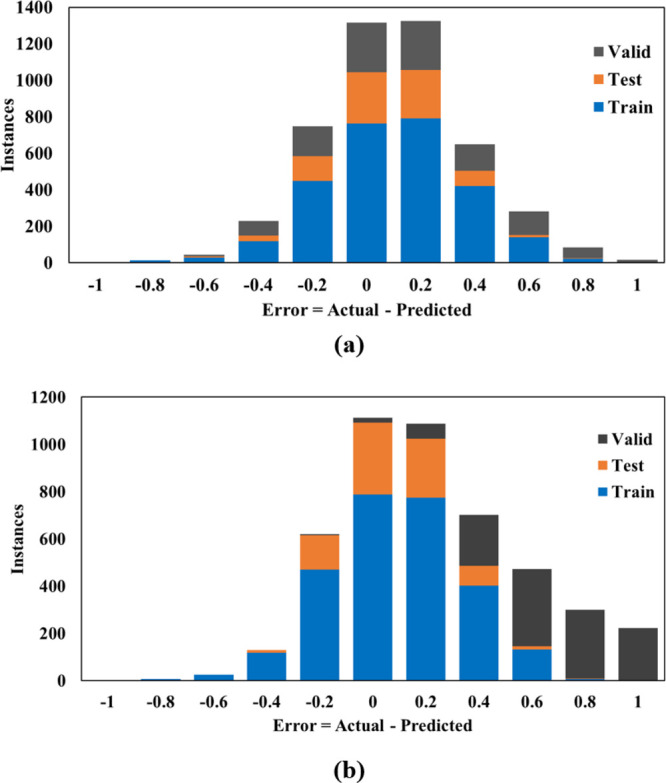
Error Histogram. (a) ANN model and (b) ANFIS model.
In addition, Figure 9 summarizes the performance of the two developed models in terms of the correlation coefficients and average absolute percentage error between the actual and predicted ECD values for training, testing, and validation data sets. It is clear that the ANN model shows a better performance than the ANFIS for estimating ECD for the validation process, as the correlation coefficient of the ANN is 0.98, while that of ANFIS is 0.96, and the AAPE of the ANN is 0.3%, while that of the ANFIS model is 0.69%.
Figure 9.
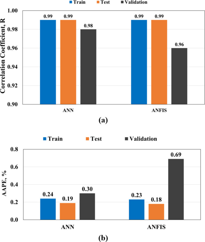
Model comparison. (a) Correlation coefficient (R) and (b) average absolute percentage error (AAPE).
The results obtained for the validation data set were compared with a recent study41 for predicting the ECD from the drilling data and found that the current models’ performance provides high accuracy, similar to that reported in a published work; the developed models in this research have an accuracy (R) range of 0.96–0.99 during the model training, testing, and validation phases, while those reported in the published work41 had a range of 0.97–0.99 using the different algorithms mentioned in the introduction part (SVM, FN, and RF). The current work presents novel contributions regarding employing different applications of AI techniques (ANN and ANFIS); besides, the current study presents a new approach toward reducing the number of the drilling parameters/inputs for the developed models by removing the hook load data from the inputs that will help to eliminate drilling issues related to the stability of the sensor measurements and uncertainty. One important finding from the current work is to provide ANN-based correlation for ECD estimation without the need for the algorithm code, which will help more the field used on the rig site for real time estimation.
Conclusions
The ECD was predicted from the real-time recordings of the surface drilling sensors by employing two different machine learning techniques (ANN and ANFIS). The input drilling data are GPM, ROP, RPM, SPP, WOB, and T. The ANN and ANFIS model parameters were optimized through different sensitivity analyses. The following conclusions represent the outputs from the work:
The study presented a new approach for predicting the ECD from the drilling data during drilling that did not require adding many models’ inputs, which will add cost, time, and uncertainty issues to the operation.
The optimization approach of each model parameters succeeded in providing a high accuracy level, as R was higher than 0.99 and AAPE was less than 0.24 for ANN and ANFIS models.
The study proved the high prediction performance through the validation process for the models that recorded R of 0.98 for ANN with 0.3% AAPE, while R was 0.96 for ANFIS with an AAPE of 0.69%.
The study developed an ANN-based equation for ECD prediction that showed high accuracy for predicting the ECD in real time without the need for the code.
The new contributions from this study will save time and cost for estimating ECD in real drilling operations, as the machine learning models were built based on the drilling data collected by the drilling sensors.
This study is limited to the data ranges for the drilling parameters and ECD, horizontal well profile, 5–7/8-inch hole section, and normal drilling operations without any downhole issues like drilling abnormal zone, cutting accumulation, and hole cleaning problems. Therefore, this study recommends further applications for different well profiles and hole sections, in addition to encountering drilled zones with abnormal pressures and other downhole drilling problems, as this will enhance the generalization of developed models for field applications.
Acknowledgments
The authors wish to acknowledge King Fahd University of Petroleum & Minerals and Rosewell Energy for permitting the publication of this work.
Glossary
Abbreviations
- ECD
Equivalent circulating density
- ANN
Artificial neural network
- ANFIS
Adaptive network-based fuzzy interference system
- R
Correlation coefficient
- AAPE
Average absolute percentage error
- AI
Artificial intelligence
- ML
Machine learning
- SVM
Support vector machine
- FN
Functional networks
- RF
Random forest
- LLSVM
Least square support vector machine
- Gaussmf
Gaussian membership function
- PSO
Particle swarm optimization
- FIS
Fuzzy Inference System
- GA
Genetic algorithm
- RBF
Radial basis function
- R2
Coefficient of determination
- MSE
Mean squared error
- RMSE
Root mean squared error
- WOB
Weight on bit
- RPM
Rotating speed in revolutions per minute
- ROP
Rate of penetration
- GPM
Gallon per minute
- SPP
Standpipe pressure
- T
Torque
- Fitnet
Function fitting neural network
- newfit
Create fitting network
- newcf
Create cascade-forward backpropagation network
- newelm
Create Elman backpropagation network
- newlrn
Layer-Recurrent Network
- Newdtdnn
Create distributed time delay neural network
- newff
Create feedforward backpropagation network
- newpr
Create pattern recognition network
- newfftd
Create feedforward input-delay backpropagation network
- trainbr
Bayesian regularization
- trainoss
One step secant backpropagation
- trainlm
Levenberg–Marquardt backpropagation
- trainbfg
BFGS quasi-Newton backpropagation
- traingdx
Gradient descent with momentum and adaptive learning rule backpropagation
- tansig
Hyperbolic tangent sigmoid transfer function
- logsig
Log-sigmoid transfer function
- hardlims
Hard-limit transfer function
- purelin
Linear transfer function
- softmax
Softmax transfer function
- tribas
Triangular basis transfer function
- satlin
Saturating linear transfer function
- netinv
Inverse transfer function
- radbas
Radial basis transfer function
Author Contributions
Conceptualization: S.E. and A.A.; methodology: A.A. and H.G.; software: A.A. and H.G.; formal analysis: A.A. and H.G.; investigation: A.A. and H.G.; data curation: S.E.; writing—original draft preparation: A.A. and H.G.; writing—review and editing: S.E.; supervision: S.E. and A.A. All authors have read and agreed to the published version of the manuscript.
The authors declare no competing financial interest.
References
- Haciislamoglu M.Practical Pressure Loss Predictions in Realistic Annular Geometries. In SPE Annual Technical Conference and Exhibition; Society of Petroleum Engineers, 1994; pp. 25–28. [Google Scholar]
- Osman E. A.; Aggour M. A.. Determination of Drilling Mud Density Change with Pressure and Temperature Made Simple and Accurate by ANN. In Proceedings of the Middle East Oil Show; Society of Petroleum Engineers (SPE), 2003; Vol. 13, pp. 115–126. [Google Scholar]
- Hemphill T.; Ravi K.. Improved Prediction of ECD with Drill Pipe Rotation. In Society of Petroleum Engineers - International Petroleum Technology Conference 2012, IPTC 2012; OnePetro, 2012; Vol. 4, pp. 3378–3383. [Google Scholar]
- Zhang H.; Sun T.; Gao D.; Tang H. A New Method for Calculating the Equivalent Circulating Density of Drilling Fluid in Deepwater Drilling for Oil and Gas. Chem. Technol. Fuels Oils 2013, 49, 430–438. 10.1007/s10553-013-0466-0. [DOI] [Google Scholar]
- Abdelgawad K. Z.; Elzenary M.; Elkatatny S.; Mahmoud M.; Abdulraheem A.; Patil S. New Approach to Evaluate the Equivalent Circulating Density (ECD) Using Artificial Intelligence Techniques. J. Pet. Explor. Prod. Technol. 2019, 9, 1569–1578. 10.1007/s13202-018-0572-y. [DOI] [Google Scholar]
- Ataga E.; Ogbonna J.; Boniface O.. Accurate Estimation of Equivalent Circulating Density during High Pressure High Temperature (HPHT) Drilling Operations. In Society of Petroleum Engineers - 36th Nigeria Annual Int. Conf. and Exhibition 2012, NAICE 2012 - Future of Oil and Gas: Right Balance with the Environment and Sustainable Stakeholders’ Participation; Society of Petroleum Engineers, 2012; Vol. 2, pp. 804–811. [Google Scholar]
- Rommetveit R.; Ødegård S. I.; Nordstrand C.; Bjørkevoll K. S.; Cerasi P.; Helset H. M.; Fjeldheim M.; Håvardstein S. T.. Drilling a Challenging HPHT Well Utilizing an Advanced ECD Management System with Decision Support and Real Time Simulations. In SPE/IADC Drilling Conference, Proceedings; Society of Petroleum Engineers (SPE), 2010; Vol. 2, pp. 849–860. [Google Scholar]
- Erge O.; Vajargah A. K.; Ozbayoglu M. E.; Van Oort E.. Improved ECD Prediction and Management in Horizontal and Extended Reach Wells with Eccentric Drillstrings. In SPE - International Association of Drilling Contractors Drilling Conference Proceedings; Society of Petroleum Engineers (SPE), January, 2016; pp. 1–3. [Google Scholar]
- Peters E. J.; Chenevert M. E.; Zhang C. A Model for Predicting the Density of Oil-Based Muds at High Pressures and Temperatures. SPE Drill Eng 1990, 5, 141–148. 10.2118/18036-PA. [DOI] [Google Scholar]
- Bybee K. Equivalent-Circulating-Density Fluctuation in Extended-Reach Drilling. J. Pet. Technol. 2009, 61, 64–67. 10.2118/0209-0064-jpt. [DOI] [Google Scholar]
- Hemphill T.; Ravi K.; Bern P.; Rojas J. C.. A Simplified Method for Prediction of ECD Increase with Drillpipe Rotation. In Proceedings - SPE Annual Technical Conference and Exhibition; Society of Petroleum Engineers (SPE), 2008; Vol. 2, pp. 1092–1098. [Google Scholar]
- Ahmed R.; Enfis M.; Miftah-El-Kheir H.; Laget M.; Saasen A.. The Effect of Drillstring Rotation on Equivalent Circulation Density: Modeling and Analysis of Field Measurements. In Proceedings - SPE Annual Technical Conference and Exhibition; OnePetro, 2010; Vol. 7, pp. 5375–5385. [Google Scholar]
- Costa S. S.; Stuckenbruck S.; Fontoura S. A. B.; Martins A. L.. Simulation of Transient Cuttings Transportation and ECD in Wellbore Drilling. In Europec/EAGE Conference and Exhibition; OnePetro, 2008. [Google Scholar]
- Caicedo H.; Pribadi M. A.; Bahuguna S.; Wijnands F.; Setiawan N. B.. Geomechanics, ECD Management and RSS to Manage Drilling Challenges in a Mature Field; Society of Petroleum Engineers (SPE), 2010. [Google Scholar]
- Kalogirou S. A. Artificial Intelligence for the Modeling and Control of Combustion Processes: A Review. Prog. Energy Combust. Sci. 2003, 29, 515–566. 10.1016/S0360-1285(03)00058-3. [DOI] [Google Scholar]
- Mohaghegh S. Virtual-Intelligence Applications in Petroleum Engineering: Part 1—Artificial Neural Networks. J. Pet. Technol. 2000, 52, 64–73. 10.2118/58046-JPT. [DOI] [Google Scholar]
- Elsafi S. H. Artificial Neural Networks (ANNs) for Flood Forecasting at Dongola Station in the River Nile, Sudan. Alex. Eng. J. 2014, 53, 655–662. 10.1016/j.aej.2014.06.010. [DOI] [Google Scholar]
- Babikir H. A.; Elaziz M. A.; Elsheikh A. H.; Showaib E. A.; Elhadary M.; Wu D.; Liu Y. Noise Prediction of Axial Piston Pump Based on Different Valve Materials Using a Modified Artificial Neural Network Model. Alex. Eng. J. 2019, 58, 1077–1087. 10.1016/j.aej.2019.09.010. [DOI] [Google Scholar]
- Rolon L.; Mohaghegh S. D.; Ameri S.; Gaskari R.; McDaniel B. Using Artificial Neural Networks to Generate Synthetic Well Logs. J. Nat. Gas Sci. Eng. 2009, 1, 118–133. 10.1016/j.jngse.2009.08.003. [DOI] [Google Scholar]
- Tariq Z.; Elkatatny S.; Mahmoud M.; Ali A. Z.; Abdulraheem A.. A New Technique to Develop Rock Strength Correlation Using Artificial Intelligence Tools. In SPE Reservoir Characterisation and Simulation Conference and Exhibition; OnePetro, 2017; Vol. 14. [Google Scholar]
- Elkatatny S.; Mahmoud M.; Tariq Z.; Abdulraheem A. New Insights into the Prediction of Heterogeneous Carbonate Reservoir Permeability from Well Logs Using Artificial Intelligence Network. Neural Comput. Appl. 2018, 30, 2673–2683. 10.1007/s00521-017-2850-x. [DOI] [Google Scholar]
- Moussa T.; Elkatatny S.; Mahmoud M.; Abdulraheem A. Development of New Permeability Formulation from Well Log Data Using Artificial Intelligence Approaches. J. Energy Resour. Technol. 2018, 140, 072903 10.1115/1.4039270. [DOI] [Google Scholar]
- Ren X.; Hou J.; Song S.; Liu Y.; Chen D.; Wang X.; Dou L. Lithology Identification Using Well Logs: A Method by Integrating Artificial Neural Networks and Sedimentary Patterns. J. Pet. Sci. Eng. 2019, 182, 106336 10.1016/j.petrol.2019.106336. [DOI] [Google Scholar]
- Ahmed A.; Ali A.; Elkatatny S.; Abdulraheem A. New Artificial Neural Networks Model for Predicting Rate of Penetration in Deep Shale Formation. Sustainability 2019, 11, 6527. 10.3390/su11226527. [DOI] [Google Scholar]
- Elkatatny S.; Mahmoud M. Development of New Correlations for the Oil Formation Volume Factor in Oil Reservoirs Using Artificial Intelligent White Box Technique. Petroleum 2018, 4, 178–186. 10.1016/j.petlm.2017.09.009. [DOI] [Google Scholar]
- Ahmed A. A.; Elkatatny S.; Abdulraheem A.; Mahmoud M.. Application of Artificial Intelligence Techniques in Estimating Oil Recovery Factor for Water Derive Sandy Reservoirs. In Society of Petroleum Engineers - SPE Kuwait Oil and Gas Show and Conference 2017; Society of Petroleum Engineers, 2017; Vol. 2, p 187621. [Google Scholar]
- Mahmoud A.; Elkatatny S.; Chen W.; Abdulraheem A. Estimation of Oil Recovery Factor for Water Drive Sandy Reservoirs through Applications of Artificial Intelligence. Energies 2019, 12, 3671. 10.3390/en12193671. [DOI] [Google Scholar]
- Elkatatny S.; al-AbdulJabbar A.; Mahmoud A. A.; New Robust Model to Estimate Formation Tops in Real Time Using Artificial Neural Networks (ANN). Petrophysics 2019, 60, 825–837. 10.30632/pjv60n6-2019a7. [DOI] [Google Scholar]
- Al-Abduljabbar A.; Gamal H.; Elkatatny S. Application of Artificial Neural Network to Predict the Rate of Penetration for S-Shape Well Profile. Arab. J. Geosci. 2020, 13, 784. 10.1007/s12517-020-05821-w. [DOI] [Google Scholar]
- Gamal H.; Elkatatny S.; Abdulraheem A.. Rock Drillability Intelligent Prediction for a Complex Lithology Using Artificial Neural Network. In Society of Petroleum Engineers - Abu Dhabi International Petroleum Exhibition and Conference 2020; ADIP, 2020. [Google Scholar]
- Alsabaa A.; Gamal H. A.; Elkatatny S. M.; Abdulraheem A.. Real-Time Prediction of Rheological Properties of All-Oil Mud Using Artificial Intelligence. In Paper presented at the 54th U.S. Rock Mechanics/Geomechanics Symposium, physical event cancelled, June 2020, https://www.onepetro.org/conference-paper/ARMA-2020-1645.
- Mahmoud A. A.; ElKatatny S.; Abdulraheem A.; Mahmoud M.; Ibrahim M. O.; Ali A.. New Technique to Determine the Total Organic Carbon Based on Well Logs Using Artificial Neural Network (White Box). In Society of Petroleum Engineers - SPE Kingdom of Saudi Arabia Annual Technical Symposium and Exhibition 2017; Society of Petroleum Engineers, 2017; Vol. 2, pp. 1441–1452. [Google Scholar]
- Mahmoud A. A.; Elkatatny S.; Ali A.; Abouelresh M.; Abdulraheem A.. New Robust Model to Evaluate the Total Organic Carbon Using Fuzzy Logic. In Society of Petroleum Engineers - SPE Kuwait Oil and Gas Show and Conference 2019, KOGS 2019; Society of Petroleum Engineers, 2019. [Google Scholar]
- Mahmoud A.; Elkatatny S.; Mahmoud M.; Abouelresh M.; Abdulraheem A.; Ali A. Determination of the Total Organic Carbon (TOC) Based on Conventional Well Logs Using Artificial Neural Network. Int. J. Coal Geol. 2017, 179, 72–80. 10.1016/j.coal.2017.05.012. [DOI] [Google Scholar]
- Mahmoud A. A.; Elkatatny S.; Al Shehri D. Application of Machine Learning in Evaluation of the Static Young’s Modulus for Sandstone Formations. Sustainability 2020, 12, 1880. 10.3390/su12051880. [DOI] [Google Scholar]
- Mahmoud A. A.; Elkatatny S.; Ali A.; Moussa T. Estimation of Static Young’s Modulus for Sandstone Formation Using Artificial Neural Networks. Energies 2019, 12, 2125. 10.3390/en12112125. [DOI] [Google Scholar]
- Tariq Z.; Elkatatny S.; Mahmoud M.; Abdulraheem A.. A Holistic Approach to Develop New Rigorous Empirical Correlation for Static Young’s Modulus. In Society of Petroleum Engineers - Abu Dhabi International Petroleum Exhibition and Conference 2016; Society of Petroleum Engineers, 2016, January. [Google Scholar]
- Elkatatny S.; Mahmoud M.; Mohamed I.; Abdulraheem A. Development of a New Correlation to Determine the Static Young’s Modulus. J. Pet. Explor. Prod. Technol. 2018, 8, 17–30. 10.1007/s13202-017-0316-4. [DOI] [Google Scholar]
- Elkatatny S.; Tariq Z.; Mahmoud M.; Mohamed I.; Abdulraheem A. Development of New Mathematical Model for Compressional and Shear Sonic Times from Wireline Log Data Using Artificial Intelligence Neural Networks (White Box). Arab. J. Sci. Eng. 2018, 43, 6375–6389. 10.1007/s13369-018-3094-5. [DOI] [Google Scholar]
- Tariq Z.; Elkatatny S.; Mahmoud M.; Ali A. Z.; Abdulraheem A.. A New Approach to Predict Failure Parameters of Carbonate Rocks Using Artificial Intelligence Tools. In Society of Petroleum Engineers - SPE Kingdom of Saudi Arabia Annual Technical Symposium and Exhibition 2017; Society of Petroleum Engineers, 2017; pp. 1428–1440. [Google Scholar]
- Alsaihati A.; Elkatatny S.; Mahmoud A. A.; Abdulraheem A. Use of Machine Learning and Data Analytics to Detect Downhole Abnormalities While Drilling Horizontal Wells, with Real Case Study. J. Energy Resour. Technol. 2021, 143, 043201 10.1115/1.4048070. [DOI] [Google Scholar]
- Arehart R. A. Drill-Bit Diagnosis With Neural Networks. SPE Comput. Appl. 1990, 2, 24–28. 10.2118/19558-pa. [DOI] [Google Scholar]
- Abdelgawad K.; Elkatatny S.; Moussa T.; Mahmoud M.; Patil S. Real-Time Determination of Rheological Properties of Spud Drilling Fluids Using a Hybrid Artificial Intelligence Technique. J. Energy Resour. Technol. 2019, 141, 032908 10.1115/1.4042233. [DOI] [Google Scholar]
- Alsabaa A.; Gamal H.; Elkatatny S.; Abdulraheem A. Real-Time Prediction of Rheological Properties of Invert Emulsion Mud Using Adaptive Neuro-Fuzzy Inference System. Sensors 2020, 20, 1669. 10.3390/s20061669. [DOI] [PMC free article] [PubMed] [Google Scholar]
- Alsabaa A.; Gamal H.; Elkatatny S.; Abdulraheem A. New Correlations for Better Monitoring the All-Oil Mud Rheology by Employing Artificial Neural Networks. Flow Meas. Instrum. 2021, 78, 101914 10.1016/j.flowmeasinst.2021.101914. [DOI] [Google Scholar]
- Elkatatny S.; Tariq Z.; Mahmoud M. Real Time Prediction of Drilling Fluid Rheological Properties Using Artificial Neural Networks Visible Mathematical Model (White Box). J. Pet. Sci. Eng. 2016, 146, 1202–1210. 10.1016/j.petrol.2016.08.021. [DOI] [Google Scholar]
- Ahmadi M. A. Toward Reliable Model for Prediction Drilling Fluid Density at Wellbore Conditions: A LSSVM Model. Neurocomputing 2016, 211, 143–149. 10.1016/j.neucom.2016.01.106. [DOI] [Google Scholar]
- Ahmadi M. A.; Shadizadeh S. R.; Shah K.; Bahadori A. An Accurate Model to Predict Drilling Fluid Density at Wellbore Conditions. Egypt. J. Pet. 2018, 27, 1–10. 10.1016/j.ejpe.2016.12.002. [DOI] [Google Scholar]
- Alkinani H. H.; Al-Hameedi A. T. T.; Dunn-Norman S.; Al-Alwani M. A.; Mutar R. A.; Al-Bazzaz W. H.. Data-Driven Neural Network Model to Predict Equivalent Circulation Density ECD. In Society of Petroleum Engineers - SPE Gas and Oil Technology Showcase and Conference 2019, GOTS 2019; Society of Petroleum Engineers, 2019. [Google Scholar]
- Rahmati A. S.; Tatar A. Application of Radial Basis Function (RBF) Neural Networks to Estimate Oil Field Drilling Fluid Density at Elevated Pressures and Temperatures. Oil Gas Sci. Technol. 2019, 74, 50. 10.2516/ogst/2019021. [DOI] [Google Scholar]
- Alsaihati A.; Elkatatny S.; Abdulraheem A. Real-Time Prediction of Equivalent Circulation Density for Horizontal Wells Using Intelligent Machines. ACS Omega 2021, 6, 934–942. 10.1021/ACSOMEGA.0C05570. [DOI] [PMC free article] [PubMed] [Google Scholar]
- Bello O.; Holzmann J.; Yaqoob T.; Teodoriu C. Application Of Artificial Intelligence Methods In Drilling System Design And Operations: A Review Of The State Of The Art. J. Artif. Intell. Soft Comput. Res. 2015, 5, 121–139. 10.1515/jaiscr-2015-0024. [DOI] [Google Scholar]
- Abbas A. K.; Rushdi S.; Alsaba M.; Al Dushaishi M. F. Drilling Rate of Penetration Prediction of High-Angled Wells Using Artificial Neural Networks. J. Energy Resour. Technol. 2019, 141, 112904. 10.1115/1.4043699. [DOI] [Google Scholar]
- Cevik A.; Sezer E. A.; Cabalar A. F.; Gokceoglu C.. Modeling of the Uniaxial Compressive Strength of Some Clay-Bearing Rocks Using Neural Network. In Applied Soft Computing Journal; Elsevier, 2011; Vol. 11, pp. 2587–2594. [Google Scholar]
- Lippmann R. P. An Introduction to Computing with Neural Nets. IEEE ASSP Mag. 1987, 4, 4–22. 10.1109/MASSP.1987.1165576. [DOI] [Google Scholar]
- Graves A.; Liwicki M.; Fernandez S.; Bertolami R.; Bunke H.; Schmidhuber J. A Novel Connectionist System for Unconstrained Handwriting Recognition. IEEE Trans. Pattern Anal. Mach. Intell. 2009, 31, 855–868. 10.1109/TPAMI.2008.137. [DOI] [PubMed] [Google Scholar]
- Elkatatny S.; Tariq Z.; Mahmoud M.; Abdulraheem A. New Insights into Porosity Determination Using Artificial Intelligence Techniques for Carbonate Reservoirs. Petroleum 2018, 4, 408–418. 10.1016/j.petlm.2018.04.002. [DOI] [Google Scholar]
- Abraham A.Adaptation of Fuzzy Inference System Using Neural Learning; Springer: Berlin, Heidelberg, 2005; pp. 53–83. [Google Scholar]