

Abstract
A cross sectional population is defined as a population of living individuals at the sampling or observational time. Cross-sectionally sampled data with binary disease outcome are commonly analyzed in observational studies for identifying how covariates correlate with disease occurrence. It is generally understood that cross-sectional binary outcome is not as informative as longitudinally collected time-to-event data, but there is insufficient understanding as to whether bias can possibly exist in cross-sectional data and how the bias is related to the population risk of interest. As the progression of a disease typically involves both time and disease status, we consider how the binary disease outcome from the cross-sectional population is connected to birth-illness-death process in the target population. We argue that the distribution of cross-sectional binary outcome is different from the risk distribution from the target population and that bias would typically arise when using cross-sectional data to draw inference for population risk. In general, the cross-sectional risk probability is determined jointly by the population risk probability and the ratio of duration of diseased state to the duration of disease-free state. Through explicit formulas we conclude that bias can almost never be avoided from cross-sectional data. We present age-specific risk probability (ARP) and argue that models based on ARP offers a compromised but still biased approach to understand the population risk. An analysis based on Alzheimer’s disease data is presented to illustrate the ARP model and possible critiques for the analysis results.
Keywords: birth-illness-death process, current status data, logistic model, sampling bias, stationary disease process
1 ∣. INTRODUCTION AND BACKGROUND
A cross sectional population is generally defined as a population of living individuals at the sampling or observational time. Cross-sectional sampling is commonly adopted by both clinical trials and observational studies. In observational studies, at the time when individuals are sampled from the cross-sectional population, the disease outcome together with the individual’s background information are also collected by the study. Such cross-sectionally sampled data with binary disease outcome are commonly analyzed for the understanding of covariate effects on the risk of contracting the disease,1,2 and this type of observational studies are the focus of this article. As the progression of a disease typically involves both time and disease status, a question of interest is how the cross-sectionally identified binary disease outcome is connected to the progression of disease and duration. Statisticians and epidemiologists generally understand that cross-sectional binary outcome is not as informative as longitudinally collected time-to-event data, but there is insufficient understanding as to whether bias can possibly exist in cross-sectional data and how the bias is related to the population risk of interest. This article presents the complexity and bias in cross-sectional data with binary disease outcome with detailed explorations into the data structure.
We consider the model setting that individuals from a birth cohort population could acquire a disease with no cure; examples include Alzheimer’s disease, Schizophrenia, HIV/AIDS, Diabetes, Cancer, and other chronic diseases. The birth cohort population is the target population of interest to understand risk factors for the disease. When studying such a disease, for those who are at the risk for the disease, an individual could contract the disease before death or die without experiencing the disease. For the understanding of risk factors or covariate effects on the risk of contracting the disease, cross-sectionally sampled data with binary disease or event outcome are commonly analyzed by the logistic models in observational studies.3,4 In use of logistic models for analyzing binary data, the sampling bias in the presence of heterogeneity was recognized and carefully studied by McCullagh.2 In this work, we study sampling bias which arises because “the choice of individuals for study is not conditionally independent of outcome given the explanatory variables,” in connection with the birth-illness-death process (quote from the discussion of McCullagh paper, by D. R. Cox); also see Lawless et al5 and Fluss et al6 for sampling biased models related to missing data and response-selective sampling.
From the target population, let the variable T be either age at incidence (or onset) of disease, or age at death if the disease did not occur during lifetime. The variable T can be viewed as time to a composite endpoint, where the endpoint is either disease incidence or death. Denote by D the individual’s age at death and R = D − T. Note that R can be interpreted as the diseased lifetime, where R = 0 if the disease did not occur during lifetime. Let X represent a p × 1 vector of baseline covariates whose value remains the same during lifetime. Define a binary variable Y = I(R > 0), where Y = 1 or 0 indicates if the disease is present or absent during lifetime. Consider cross-sectional sampling to observe a binary variable, Y*, at calendar time s, with possible values 1 and 0 which, respectively, indicates an individual’s diseased or disease-free status. Let X*, T*, and D*, respectively, denote the sampling versions of X, T, and D in the cross-sectional population. Let W* denote the age of a cross-sectionally sampled individual at the sampling time. Clearly W* is not a baseline variable so we use a separate notation and do not treat it as an entry in the covariate vector X*.
A question of interest is whether the cross-sectionally observed variable Y* can be used to replace Y to study the lifetime risk associated with covariates in the target population. And, if the answer is no, could we learn risk of some sort from the observed Y*? Before we explore and address these questions, there is actually sufficient evidence to suggest that Y* may not lead to valid analysis for lifetime risk in view of the well know length-bias phenomenon in cross-sectional population: Under the stationarity condition (which will be discussed in later sections), if individuals are randomly selected from the cross-sectional population then conditional on X* = x, D* is distributed with the length bias density
| (1) |
and W* conditional on X* = x is distributed with the density
| (2) |
where fD(d; x) and SD(w; x), respectively, are the density and survival functions of D given X = x. The formulas in Equations (1) and (2) are known as the density function for length bias distribution and the density function of backward recurrence time.7,8 With the density formulas (1) and (2), it is clear that the cross-sectional population comprises individuals with lifetime distribution stochastically larger than that of the target population, which implies that the target population structure is not reflected by the cross-sectional population. The complexity of cross-sectional sampling, directly or indirectly related to length bias, arises in observational studies, but unfortunately it is often ignored or unrecognized by practitioners or even statisticians. As a result, cross-sectional data with binary disease outcome are commonly analyzed by the “usual” analytical approaches, such as logistic regression, but inappropriately interpreted referring to the target population parameters. A data example is included in Section 6.2 with the target population formed by individuals with Down Syndrome (DS) who were known to have high risk for developing Alzheimer’s disease. We will use this data example to illustrate the bias of cross-sectional data analyses.
As the progression of a disease typically involves disease status and duration, in this article we study how the cross-sectionally sampled binary disease outcome, Y*, is connected to Y through failure times T and R. As will be shown in Section 2, the distribution of Y* is determined not only by the population distribution of Y but also jointly by the distribution of (T, R). In Section 3, we connect the logistic regression model to the cross-sectional binary outcome Y* and the failure time distribution of (T, R). In general, bias is present in the logistic model on the basis of cross-sectional binary outcome, and, depending on the failure time structure of (T, R), the inferential results could be very biased or even with opposite effects for identifying risk factors or covariates. While the bias does not seem avoidable in the logistic model, a question of interest is whether it is possible to obtain relevant inferential properties from binary disease data in a cross-sectional study. Section 4 explores age-specific conditional inference and discusses a compromised model on the basis of an age-specific risk probability (ARP). Regardless that this compromised model is widely used in data applications, in Section 5, we argue that the ARP involved in the model is biased and frequently misinterpreted. A small simulation together with an analysis based on Alzheimer’s disease data are presented in Section 6. The article is concluded with a discussion in Section 7.
2 ∣. BIAS FROM CROSS-SECTIONAL DATA
2.1 ∣. Population dynamics and disease process
Consider population dynamics in which individuals in a target population may develop a disease over time and subsequently die. For those individuals with covariates X = x, let Bx(u) represent a population-level continuous point process, where Bx(u) is the total number of births occurring in he calendar time interval [0, u], u ≥ 0. Let Tu and Du respectively denote the disease-free time and lifetime of the individual born at calendar time u.
Let λ(u; x), u > 0, be the birth rate function for dBx(u), where the rate function has the direct interpretation as the average count of births per unit time given x, λ(u; x)du = E[dBx(u)]. Let STu(t; x) be the survival function of Tu, given X = x, for those individuals born at calendar time u. Denote by I(·) the indicator function with binary values 0 and 1. At a large and fixed calendar time s, define
as the total number of living individuals, with covariates X = x, who remained disease-free at calendar time s. Furthermore, note that
implies
| (3) |
where E{Nx(s)} is the rate of disease-free individuals at calendar time s. At a large and fixed calendar time s, for those individuals with X = x, define the second point process
which is the total number of living individuals with covariates X = x at calendar time s.
In applications, the calendar time s plays the role as a sampling time for collecting disease status data. Let SDu (t; x) be the survival function of Du given X = x, for those individuals born at u. Using procedures similar to those for deriving formula (3), one can derive
| (4) |
Formulas (3) and (4) together provide a base for understanding the dynamics of disease population, and with additional assumptions they lead to simplified properties as will be discussed below. Further assume the following stationary condition of the birth-illness-death process:
Assumption 1. Assume the birth process Bx(u) has constant birth rate: λ(u; x) = λ0,x, an x-dependent positive constant.
Assumption 2. The survival distributions STu (t; x) and SDu (t; x) are independent of an individual’s birth time u.
Assumptions 1 and 2 together are referred to as the stationarity condition of the birth-illness-death process. The two assumptions imply that the birth-illness-disease process has reached an equilibrium condition where the rates of birth, disease incidence, and disease prevalence are all constant over the calendar time. Here we indicate that A1 and/or A2 could be violated when, for instance, the birth rate increased over time because the population grew with increased number of immigrants, the human lifetime is prolonged because of advances of medicine, or a new treatment became available to delay the onset time of disease or reduce the occurrence rate of disease. Under Assumption 2, to simplify notations, the u-dependent bivariate failure times Tu and Du are expressed as T and D, and the survival functions STu (t; x) and SDu (t; x) are, respectively, expressed as ST(t; x) and SD(t; x). Suppose both T and D have finite support in distribution, and suppose the birth-illness-disease process has taken place from a remote past so that the calendar time s, for sampling, is larger than the upper bounds of support of T and D. Let Ex(D) = E{D∣X = x} and Ex(T) = E{T∣X = x}. Under Assumptions 1 and 2, formulas (3) and (4) are simplified as
| (5) |
| (6) |
In formula (5), E{Nx(s)} is the average count of disease-free individuals with X = x at calendar time s, which coincides with the product of the birth rate and expectation of disease-free lifetime. In contrast, in Equation (6), E{Mx(s)} is the average count of living individuals with X = x, diseased or disease-free, at calendar time s, which is the product of the birth rate and expectation of lifetime. The probability procedures we used here to derive Equations (5) and (6) are similar to those for deriving the well known formula Prevalence = Incidence × Duration; see, for example, Rhame and Sudderth,9 Zhu and Wang,10 and Shinohara et al.11 These formulas can also be obtained using a framework based on disease incidence and prevalence in the Lexis diagram as described by Keiding.12
Suppose the binary outcome variable Y* is sampled at calendar time s, where s does not carry information for the bivariate times T and R from the study individual. Then, at sampling time s and conditional on covariates X* = x, the risk-free probability for a randomly sampled individual is the cross-sectional proportion of disease-free individuals among all the living individuals at s:
Thus,
| (7) |
| (8) |
The risk-free and risk probabilities in Equations (7) and (8) are essentially the fractions of an individual’s average disease-free and diseased duration in lifetime. Let βx = Ex(T) and γx = Ex(R∣R > 0), respectively, denote the average length of disease-free time, and average length of diseased times among the diseased individuals. It follows that
| (9) |
| (10) |
Clearly P(Y* = 1 ∣ X* = x) ≠ P(Y = 1 ∣ X = x), which implies that an enforced logistic regression model on a set of independent and identically distributed cross-sectional observations , collected at calendar times s1, … , sn, will result in biased analysis for the true model for Y.
2.2 ∣. Bias in absolute and relative risks
It is clearly seen that, from Equations (9) and (10), the cross-sectional risk probability P(Y* = 1 ∣ X* = x) is determined jointly by the population risk probability, P(Y = 1 ∣ X = x), and the ratio of diseased duration to the disease-free duration, . By simple algebra, the relationship between the cross-sectional risk probability and the population risk probability is stated in the following proposition.
Proposition 1. The cross-sectional risk probability is related to the population risk probability through the following condition: P(Y* = k ∣ X* = x) = P(Y = k ∣ X = x), k = 0, 1, if and only if .
Clearly, Proposition 1 does not hold if βx > γx, since P(Y = 0 ∣ X = x) can not exceed 1. In general, the cross-sectional risk probability is rarely the same as the population risk probability even if βx ≤ γx. Also, P(Y* = 0 ∣ X* = x) > (or <) P(Y = 0 ∣ X = x) if and only if P(Y = 0 ∣ X = x) < (or >) , which implies that the direction of bias is determined by the ratio of disease-free duration to the diseased duration. Thus, in general, the bias from cross-sectional binary outcome variable is present and there is no guarantee that risk factors in the population risk model are properly reflected in the cross-sectional model when studying the absolute risk probability of the disease.
A question of interest now is whether the relative risk is also biased. To examine the bias of relative risk, express the sampling relative risk as
| (11) |
The following two special cases could be of interest:
Consider a rare disease model where P(Y = 1 ∣ X = x) ≈ 0. Suppose the duration ratio is not too extreme that is, not close to 0 or ∞). Then, the third curly bracket term in (11) is approximately 1, the S.R.R. is approximately the product of the first and second terms, and the bias in S.R.R. is mostly determined by the second curly bracket term in (11), that is, the ratio of to . The S.R.R. is approximately unbiased if .
-
In case the ratio of of diseased duration to the disease-free duration, , is independent of x, then
(12) which implies that, no matter if S.R.R. is larger or smaller than 1, the cross-sectional effect from S.R.R. is always diminished because the first and second curly bracket terms in Equation (12) always take the opposite directions in magnitude for relative effect; that is, ∣S.R.R. − 1∣ ≤ ∣R.R. − 1∣. However, if the population R.R. = 1, then both the first and second curly bracket terms equal 1 and the bias of S.R.R. reduces to zero. In this case, the S.R.R. in the cross-sectional data is unbiased, even though the absolute risk could still be biased.
In general, the bias is jointly determined by the ratio of disease-free duration to the diseased duration and the risk probability, as seen from the formula below:
3 ∣. SAMPLING BIAS AND LOGISTIC MODEL
In this section, we consider the logistic model to examine the bias from cross-sectional data. Suppose the logistic regression model holds for the population disease indicator Y = I(R > 0), conditional on covariates X, with risk probability
where α0 is a scalar parameter and α = (α1, … , αp)′ is a p × 1 vector of parameters. Conditional on X* = x, we will show that the distribution of Y* is determined not only by P(Y = 1 ∣ X = x), but also by the distribution of bivariate failure times T and R. The risk probability for Y* is
It is clear to see P(Y* = 1 ∣ X* = x) =, < or > P(Y = 1 ∣ X = x) if and only if .
As seen from above, the ratio of diseased duration to the disease-free duration, , determines the direction and amount of bias from the risk probability P(Y* = 1 ∣ X* = x) from cross-sectional data. For example, in the case of rare disease where exp(α0 + α′x) ≈ 0, the cross-sectional risk probability P(Y* = 1 ∣ X* = x) would be smaller (larger) than the population risk probability P(Y = 1 ∣ X = x) when the average length of diseased time γx is shorter (longer) than the disease free-time βx. The sampling odds ratio is
| (13) |
In general, the bias of odds ratio is present if the product of the two curly bracket terms in Equation (13) is not 1. We consider two situations:
-
When the disease is rare, P(Y = 0 ∣ X) ≈ 1, formula (13) can be expressed as
and the ratio of to determines the bias of odds ratio.
-
In the case that the ratio of of diseased duration to the disease-free duration, , is independent of x, formula (13) reduces to
which is an interesting result in comparison with ∣S.R.R. − 1∣ ≤ ∣R.R. − 1∣ under formula (12). Noting that, with the additional condition that the disease is rare, one further obtains S.O.R. = R.R. ≈ O.R.
In many studies, the cross-sectional sampling is restricted to a specified age range of individuals from a1 to a2, a1 < a2; say 40~60 years of age. That is, at sampling time si, i = 1, … , n, an individual with is randomly sampled from the group of individuals with ages a1 ~ a2. For these studies with age specification, the discussion and formulas established in Section 2 still hold but the definitions of D, T need to be respectively modified by conditioning on the sub-population of individuals with lifetime and disease-free time between ages a1 and a2. Also, the variable R = D − T will be modified as the diseased time between ages a1 and a2, and Y = I(D > T) modified as the indicator only for those individuals with disease incidences between ages a1 and a2. All the formulas derived for the logistic model in this section also extend to the revised population, which is subject to age constraint.
When the stationarity condition (specified by Assumptions 1 and 2) is not satisfied, the model is referred to as a non-stationary model in which, in general, formulas in Equations (5)~(8) do not hold. Although it is less clear how the cross-sectional risk probability is related to the population risk probability, there is no reason why one should expect the cross-sectional data analysis to be unbiased.
4 ∣. AGE-SPECIFIC RISK PROBABILITY AND LOGISTIC MODELS
In Sections 2 and 3, using the covariates X* defined at baseline (birth), the bias does not seem avoidable for the estimation of lifetime risk. In many studies, a regression model would typically include individual’s age at cross-sectional sampling time as a covariate besides the baseline covariates. In this section, we consider an ARP and argue that models based on this risk probability offers a compromised but still biased approach to understand the population risk—it is considered a compromised approach because the ARP is expressed in an explicit manner as the risk probability, but the approach still involves bias due to the cross-sectional sampling of survivors.
Recall that T* and D*, respectively, denote the sampling versions of T and D in the cross-sectional population, and W* denotes a cross-sectionally sampled individual’s age at sampling time. The variable W* will be treated as a conditional statistic when modeling the binary outcome Y*, but, as will be seen below, its role is quite different from the baseline covariates X*. Under Assumption 2 and conditioning on (W*, X*) = (w,x), the risk-free and risk probabilities in the cross-sectional population can be, respectively, expressed as
Thus, the probability density function of Y*(= y) given (W*,X*) = (w,x) is
| (14) |
where, clearly, 0 ≤ ST(t)/SD(t) ≤ 1 for each t. The risk-free probability in formula (14), η(w; x) = ST(w; x)/SD(w; x), is interpreted as the probability that a living individual with age W* = w remains disease-free (Y* = 0) given covariates X* = x. Clearly η(w; x) is age-dependent and the ARP is defined as 1 − η(w; x).
The validity of densities in Equations (9)~(13) relies on Assumptions 1 and 2 and requires that an individual’s age, W*, be truly randomly sampled from the cross-sectional population. As a contrast, the validity of the conditional density in Equation (14) requires only Assumption 2, which implies the density formula in Equation (14) holds in situations that the birth process has a non-constant rate over calendar time or that the study employs stratified sampling to sample individuals in different age groups.
An important feature of the ARP is that it is defined conditional on an individual’s survivorship at a specific age w; therefore, the underlying population for interpreting the ARP changes over chronological ages. On the basis of independently distributed cross-sectional observations, , the likelihood function is
| (15) |
If a logistic function is used to model the ARP, either parametric or semiparametric logistic models could be considered:
A standard parametric model with logit {1 − η(w; x)} = α0 + α′x + θw, where θ, α0 are scalar parameters, and α is a p × 1 vector of parameters.
A semiparametric model with logit {1 − η(w; x)} = α′x + ϕ(w), where ϕ(·) is a nonparametric function.
Of note, Model 1 is widely adopted as the standard logistic regression model by practitioners for data analysis. For Model 1, the ARP is monotone in w given x, and the standard maximum likelihood estimation approach can be employed for estimation inference. For Model 2, we can adopt either the semiparametric approach of Severini and Staniswalis13 or the method developed for the proportional odds model14 for statistical analysis. In Section 6, we will present a data example and logistic regression analysis based on these two models.
The ARP models possess additional advantages that they require less restrictive assumptions. In the case that the validity of Assumption 1 is violated or questionable and only Assumption 2 is satisfied, the ARP models can be readily used since the validity of ARP requires only the condition specified in A2. In the situation that Assumptions 1 and 2 are both violated, the ARP models would still be relevant as long as an individual’s birth time, u, is treated as a covariate and properly modeled in SD and ST, and subsequently included as a covariate in the ARP as 1 − η(w; x, u).
As the ARP is defined conditionally on survivorship at a specified age, a question arises naturally as to whether age-dependent covariates collected at the sampling time, w*, can be used in the regression model. Conceptually, since the value of y* indicates the absence or presence of disease at age w*, age-dependent covariates x*(w*) cannot serve as a causal factor for y*, even though it can still be included in the model to study its association with the ARP at age w*.
5 ∣. INTERPRETATION BIAS IN ARP MODELS AND POSSIBLE EXTENSIONS
5.1 ∣. Interpretation bias
While the logistic models, especially Model 1, are commonly adopted to analyze cross-sectional binary data, the models can only draw inferences of η(w; x) and cannot be used to identify the structure of T. For example, at a specific age w, low risk for T (ie, large value of ST(w; x)) with long lifetime D (ie, large values of SD(w; x)) is not distinguishable from high risk for T (ie, small values of ST(w; x)) with short lifetime D (ie, small value of SD(w; x)) since η(w; x) = ST(w; x)/SD(w; x). Essentially, because the cross-sectional population tends to have larger probability to include individuals with longer lifetime, the risk structure of the failure time T is not identifiable by cross-sectional data.
For the special case D = ∞ (ie, SD(w; x) = 1), clearly η(w; x) = ST(w; x) and the likelihood in Equation (15) reduces to
which is a familiar likelihood function based on current status data for the distribution of T; see Jewell and van der Laan15 for a complete review on methods and inference for current status data. In these cases, the ARP reduces to 1 − ST(w; x) and the coresponding data analysis would be appropriate and bias-free. For examples, in some studies the disease is not fatal and the diagnosis of disease takes place long before death. In these situations, the event of death can be ignored by setting D = ∞. Typical studies include child diseases such as measles, autism and attention deficit hyperactivity disorder (ADHD).
In the general setting where the event of death is not ignorable, it is clear η(w; x) ≠ ST(w; x) and the risk identified from cross-sectional data is 1 − η(w; x), not 1 − ST(w; x). In general, cross-sectional binary data can be used to identify η(w; x) but not ST(w; x), because ST and SD in η(w; x) are not distinguishable by cross-sectional data. In most data applications, the risk probability of T, 1 − ST(w; x), is of primary interest and it is under-estimated by the ARP. Unfortunately, in biomedical data applications, there is insufficient understanding of the interpretation bias related to the logistic and other regression models (such as probit model). As most practitioners may not understand what the ARP models can really estimate, interpretation of the ARP models could be problematic or even misleading.
5.2 ∣. Estimation with extended data
Some of the population functionals such as survival function of T, cause-specific hazard functions or cumulative incidence functions for time to competing events (disease incidence, disease-free death) possess nice features for interpretation. Unfortunately, these functionals cannot be estimated when cross-sectional binary data are the only data available to investigators.
In some situations, when extended information or data become available, bias could be avoided by using additional analytical procedures. For example, in the case that SD is estimable (or known) from extended data, let denote an estimate of SD and derive the estimate using the logistic models 1 or 2 based on cross-sectional data. Then, we can obtain an estimate and examine the influence of individuals’ survivorship in ARP from the cross-sectional population. In observational studies, investigators might adopt the design to recruite a cross-sectional sample for initial data analysis, then extend the study to follow individuals over time to collect time to disease and death data. In such cases, the observation of time to death is subject to left truncation and right censoring, and the follow-up data can be used to estimate the distribution SD. In Section 6.2, we will give an illustration of such analyses using a real data example.
6 ∣. SIMULATION AND A DATA EXAMPLE
6.1 ∣. Simulation
A small simulation study is conducted to examine formula (13) and to identify bias of the sampling odds ratio from cross-sectional data {(X*, Y*)} with the underlying true distribution of {(X, Y)} generated by a logistic regression model.
X is generated by Bernoulli distribution with success probability 0.4. The true model for Y is logit P(Y = 1∣X) = α0 + α1X with parameter values α0 = 0.6, α1 = 0.3.
Generate T ~ Weibull(2, 3 + X). If Y = 0, then set R = 0; when Y = 1, then generate R ~ Gamma(10, 1 + X). Set D = T + R.
Generate W ~ Unif(0, 25), which is the so-called truncation distribution16 and corresponds to the birth distribution over calendar time. The stationarity condition is ensured by the choice of uniform distribution. The support of W is set to be large enough to cover the maximum of simulated values of T and D. Noting that theoretically there is a small probability that D > W (and T > W), but it is negligible and can be treated as 0 in the simulation.
Discard data with D < W and keep those observations which satisfy D ≥ W, where the notation (D*, W*) is used to represent the untruncated data. Use the untruncated {(X*, Y*)} to fit logistic regression. Note that the untruncated observations, {(X*, Y*)}, form the cross-sectional sample in reality.
In each simulation, a large sample {(X, Y, T, R, W)} is generated to begin with by setting sample size = 1000, and we randomly sample n = 200 individuals from those untrucated observations satisfying D ≥ W to fit logistic regression. The simulation is replicated 1000 times.
Theoretical values: β0 = 2.66, β1 = 3.55, γ0 = 10, γ1 = 5.
In contrast with the true value α1 = 0.3, the theoretical value of the log sampling odds ratio (S.O.R.) can be calculated using Equation (13) as . From 1000 replicated simulations, the average of the MLE of S.O.R. is −0.885 (with s.e. 0.321). This simulation showed that there was even a sign change in the log odds ratio and suggested that use of the S.O.R. could be in serious error. This simulation study validates formula (13) and suggests that using cross-sectionally sampled data to draw conclusion could lead to very biased results. Note that for binary X the MLE is also the empirical distribution estimates, which explains why the average value of MLE is close to the theoretical value of S.O.R. For general p-dimensional covariates X, the logistic model does not generally hold for cross-sectional data and the MLE may not even converge to the sampling S.O.R.
6.2 ∣. A data example
In Alzheimer’s Disease (AD) research, cross-sectional and longitudinal sampling designs are commonly employed to study risk factors or biomarkers which predict or are associated with the development of AD. When analyzing cross-sectional data, binary disease outcome based on the presence or absence of AD is commonly treated as unbiased data and analyzed by standard approaches. In this section, using both covariates X* and cross-sectionally defined age W*, we conduct data analyses based on the two ARP models described in Section 4.
Adults with DS are generally known to have high risk for developing AD.17 In an ADDS Study, a group of individuals with DS were recruited to neurology specialty clinics in the greater Boston area. We analyzed data from 557 adults who were 25 to 70 years old at the time of the initial visit. The study individuals lived in institutions for the developmentally disabled, or group or private homes in the community at their first visit. Based on information from all sources, AD related dementia was determined at the first visit, which defined the cross-sectional binary outcome Y*. We used the two ARP models described in Section 4, which included an individual’s age at initial visit (), sex ( for women, 0 for men), and Apolipoprotein E4 ( for those with allele 3/4 or 4/4, and 0 with allele 2/2, 2/3, or 3/3) on risk of developing AD:
Model 1:
Model 2: , where ϕ(·) is an unknown nonparametric function.
In the construction of Models 1 and 2, initially the interaction term was included; it is removed from the models because the interaction term was not significant. Using the maximum likelihood estimation approach, the intercept and regression coefficients for sex, APOE4 (Apolipoprotein E4) and age were respectively estimated by (s.e. = 1.12), (s.e. = 0.26), (s.e. = 0.31), and (s.e. = 0.02). The analysis suggested that women have higher risk (adjusted odds ratio) for developing AD, APOE4 is positively associated with risk of AD but the risk is not significant, and age is positively and strongly associated with the risk of AD.
To conduct the semiparametric analysis for Model 2, we used an algorithm in R package “GPLM” developed by Müller,18 which is a simplified version of the iterative algorithm proposed by Severini and Staniswalis:13 Two bandwidths are used for estimating ϕ(w): 5 years and 8 years. When 5 years is chosen as the bandwidth, the analysis results in (s.e. = 0.25) and (s.e. = 0.31), which are similar to the analysis result when bandwidth is set as 8 years: (s.e. = 0.25) and (s.e. = 0.30). With 5 years and 8 years as the selected bandwidths, in Figure 1 the baseline ARP, exp{ϕ(w)}/[1 + exp{ϕ(w)}], is estimated at different ages (w). The baseline ARP is interpreted as the probability of having developed AD for men with negative APOE4 given survivorship at age w.
FIGURE 1.
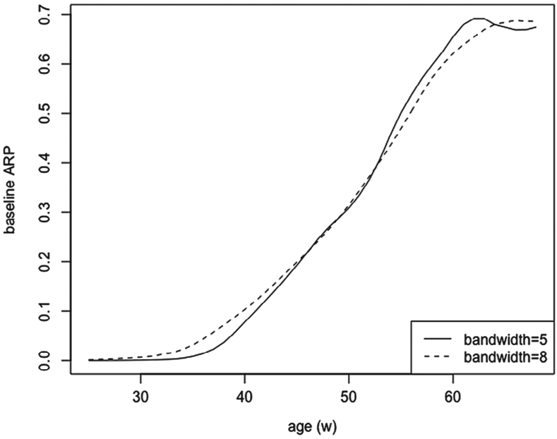
Baseline age-specific risk probability
The two (parametric or semiparametric) models conclude similar analysis results: The APOE4 genotyping confers greater AD risk but the effect does not appear significant, and women tend to have higher risk for developing AD. The two functional estimates, , are presented in Figure 1, which are seen approximately linear from age 40 to 60, and show nonlinear effect for age below 40 or above 60.
The ARP function in Model 2 is defined as
with ϕ(·) a nonparametric function. Under Model 2, we also plot out the ARP curves in Figure 2 for four different groups: women with APOE4+, women with APOE4−, men with APOE4+, men with APOE4−. The four groups, respectively, are labeled by , and (0,0).
FIGURE 2.
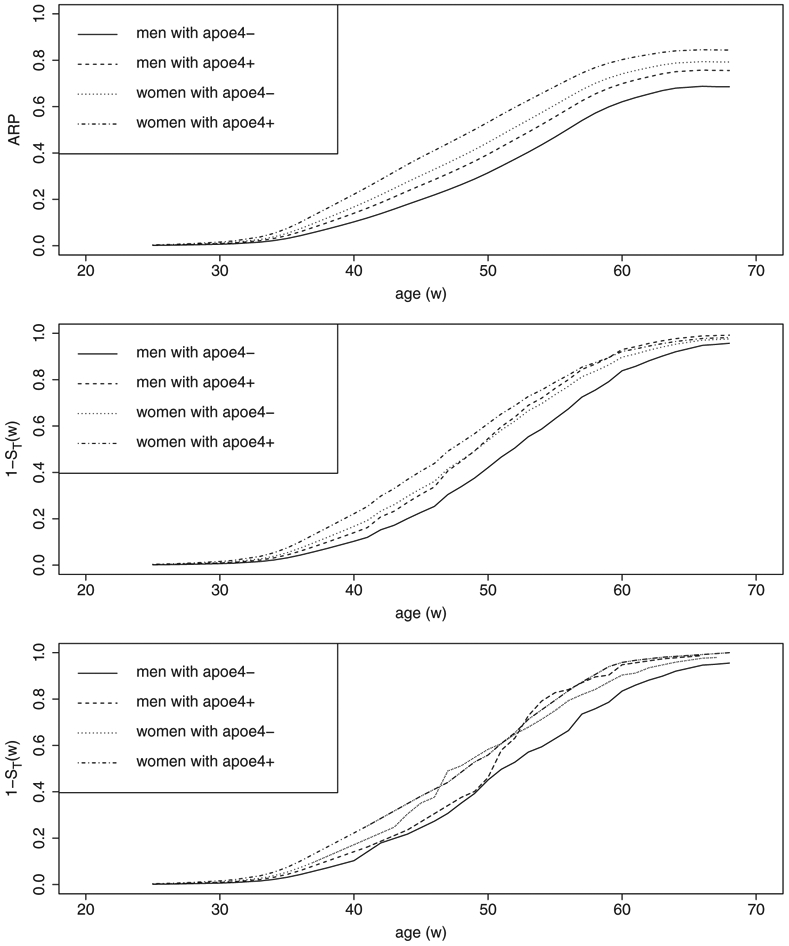
The ARP curves (top panel). Curves of 1 − ST(w) derived by the Cox model (middle panel). Curves of 1 − ST(w) derived by the nonparametric product-limit estimator (bottom panel)
As we indicated at the end of Section 5, the interpretation on the basis of ARP could be regarded as a compromised version of risk probability, with the hope that the ARP, 1 − η(w; x), is close to 1 − ST(w; x). Nevertheless, without additional source of data information, it is unlikely to examine the difference between 1 − η(w; x) and 1 − ST(w; x). In reality, when cross-sectional data are the only data available to investigators, it is important to recognize the limitation of the ARP model so that the model can be properly interpreted.
The ADDS Study actually collected both cross-sectional and longitudinal follow-up data, including the data information of age-at-death which was subject to left-truncation and right-censoring. The additional data allowed us to examine the difference between 1 − η(w; x) and 1 − ST(w; x). The age-at-death data can be used to obtain an estimate of SD(w; x), . Using and an estimate from the cross-sectional data, we obtain an estimate . Thus, the two risk probabilities 1 − η(w; x) and 1 − ST(w; x) can be compared via their estimates to examine the influence of individuals’ survivorship in ARP from the cross-sectional population.
We estimated the distribution of SD for each of the four groups labeled by using two approaches: (i) Cox regression model, , and (ii) nonparametric product-limit estimator for left-truncated and right-censored data; then obtained estimates of 1 − ST(w; x) by . In the first plot of Figure 2, women with APOE4+ and women with APOE4− had the highest and second highest ARP. Interestingly, when the ARP was replaced by 1 − ST(w; x) in the second plot, the order of the four risk groups changed and men with APOE4+ were ranked the second highest risk group after age 50. The order of the four risk groups fluctuated over lifetime in the third plot, probably due to the lack of stability of nonparametric estimator in estimation.
The data that support the findings in this section were made available to the authors by investigators of the ADDS Study, which is funded by the National Institute on Aging in the United States. Restrictions apply to the availability of these data, which were used under license for this study.
7 ∣. CONCLUSION AND RECOMMENDATION
This article studies and provides analytical explanations on how a binary disease outcome from cross-sectional population is connected to birth-illness-death process in the target population. We compare the risk probabilities, for the binary outcome, from the target population and the cross-sectional population. We argue that bias can almost never be avoided from cross-sectional data and derive bias formulas for absolute risk, relative risk, and odds ratio.
Study designs with cross-sectional binary disease outcome are commonly adopted for exploratory analysis to understand risk patterns of disease occurrence. A question of interest, under either stationary or non-stationary models, is how to correct bias from cross-sectional data with binary outcome and how to conduct unbiased statistical analysis. While the question may not have a completely satisfactory answer, in this article, using the information of individual’s age at sampling time, we study the ARP-based models which offer somewhat compromised interpretation for the risk probability of the binary disease outcome. To conclude this article, we summarize our research findings:
It is important to recognize that individuals in a cross-sectional population tend to have longer lifetime than individuals in the target population. The risk distribution of the cross-sectional population is generally different from the risk distribution of the target population.
In a stationary disease model, the cross-sectional risk and risk-free probabilities are determined jointly by the population risk probability and the ratio of duration of diseased state to the duration of disease-free state, which are explicitly expressed in Equations (9) and (10).
Conditional on baseline covariates X*, bias formulas are derived for absolute risk, relative risk, and odds ratio in Equations (9)~(13). We conclude that bias is not avoidable from cross-sectional data analysis unless deaths are negligible in the cross-sectional sample.
Conditional on both baseline covariates (X*) and an individual’s age at sampling time (W*), the ARP model serves as a compromised approach for understanding the population risk. It is important to understand that this compromised model could be easily criticized because the definition of ARP is conditional on survivorship at the time of cross-sectional sampling after the incidence of disease.
Since bias is hardly avoidable, investigators should be cautious when attempting to use cross-sectional data to understand the risk of a disease. In contrast with a cross-sectional sampling design, a longitudinal follow-up study to collect time to disease data would be much more relevant for the understanding of disease patterns and risks.
DATA AVAILABILITY STATEMENT
The data that support the findings in this section were made available to the authors by investigators of the ADDS Study, which is funded by the National Institute on Aging in the United States. Restrictions apply to the availability of these data, which were used under license for this study.
REFERENCES
- 1.Cox DR, Snell EJ. Analysis of Binary Data. Vol 32. Boca Raton, FL: CRC Press; 1989. [Google Scholar]
- 2.McCullagh P Sampling bias and logistic models. J Royal Stat Soc Ser B (Stat Methodol). 2008;70(4):643–677. [Google Scholar]
- 3.Cox DR. The regression analysis of binary sequences. J Royal Stat Soc Ser B. 1958;20:215–242. [Google Scholar]
- 4.Walker SH, Duncan DB. Estimation of the probability of an event as a function of several independent variables. Biometrika. 1967;54(1–2):167–179. [PubMed] [Google Scholar]
- 5.Lawless J, Kalbfleisch J, Wild C. Semiparametric methods for response-selective and missing data problems in regression. J Royal Stat Soc Ser B (Stat Methodol). 1999;61(2):413–438. [Google Scholar]
- 6.Fluss R, Mandel M, Freedman LS, et al. Correction of sampling bias in a cross-sectional study of post-surgical complications. Stat Medic. 2013;32(14):2467–2478. [DOI] [PubMed] [Google Scholar]
- 7.Feller W An Introduction to Probability Theory and Its Applications. Vol 1. New York, NY: John Willey & Sons; 1968. [Google Scholar]
- 8.Cox D Some Sampling Problems in Technology. New Developments in Survey Sampling. New York, NY: Wiley Interscience; 1969. [Google Scholar]
- 9.Rhame FS, Sudderth WD. Incidence and prevalence as used in the analysis of the occurrence of nosocomial infections. Am J Epidemiol. 1981;113(1):1–11. [DOI] [PubMed] [Google Scholar]
- 10.Zhu H, Wang MC. Analysing bivariate survival data with interval sampling and application to cancer epidemiology. Biometrika. 2012;99(2):345–361. [DOI] [PMC free article] [PubMed] [Google Scholar]
- 11.Shinohara RT, Sun Y, Wang MC. Alternating event processes during lifetimes: population dynamics and statistical inference. Lifetime Data Analysis. 2018;24(1):110–125. [DOI] [PubMed] [Google Scholar]
- 12.Keiding N. Age-specific incidence and prevalence: a statistical perspective. J Royal Stat Soc Ser A (Stat Soc). 1991;154(3):371–412. 10.2307/2983150. [DOI] [Google Scholar]
- 13.Severini TA, Staniswalis JG. Quasi-likelihood estimation in semiparametric models. J Am Stat Assoc. 1994;89(426):501–511. [Google Scholar]
- 14.Rossini A, Tsiatis A. A semiparametric proportional odds regression model for the analysis of current status data. J Am Stat Assoc. 1996;91(434):713–721. [Google Scholar]
- 15.Jewell NP, van der Laan M. Current status data: review, recent developments and open problems. Handbook Stat. 2003;23:625–642. [Google Scholar]
- 16.Wang MC. Nonparametric estimation from cross-sectional survival data. J Am Stat Assoc. 1991;86(413):130–143. [Google Scholar]
- 17.Wisniewski T, Castano EM, Golabek A, Vogel T, Frangione B. Acceleration of Alzheimer’s fibril formation by apolipoprotein E in vitro. Am J Pathol. 1994;145(5):1030. [PMC free article] [PubMed] [Google Scholar]
- 18.Müller M. Estimation and testing in generalized partial linear models? a comparative study. Stat Comput. 2001;11(4):299–309. [Google Scholar]
Associated Data
This section collects any data citations, data availability statements, or supplementary materials included in this article.
Data Availability Statement
The data that support the findings in this section were made available to the authors by investigators of the ADDS Study, which is funded by the National Institute on Aging in the United States. Restrictions apply to the availability of these data, which were used under license for this study.