Improving Docking Power for Short Peptides using Random Forest

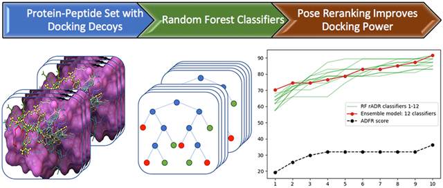
Abstract

In recent years, therapeutic peptides (TPs) have gained a lot interest as demonstrated by the 60 peptides approved as drugs in major markets and 150+ peptides currently in clinical trials. However, while small molecule docking is routinely used in rational drug design efforts, docking peptides has proven challenging partly because docking scoring functions, developed and calibrated for small molecules, perform poorly for these molecules. Here, we present Random Forest classifiers trained to discriminate correctly docked peptides. We show that, for a testing set of 47 protein-peptide complexes, structurally dissimilar from the training set and previously used to benchmark AutoDock Vina’s ability to dock short peptides, these Random Forest classifiers improve docking power from ~25% for AutoDock scoring functions to an average of ~70%. These results pave the way for peptide-docking success rates comparable to those of small molecule docking. To develop these classifiers, we compiled the ProptPep37_2021 dataset, a curated, high-quality set of 322 crystallographic protein-peptides complexes annotated with structural similarity information. The dataset also provides a collection of high-quality putative poses with a range of deviations from the crystallographic pose, providing correct and incorrect poses (i.e., decoys) of the peptide for each entry. The ProptPep37_2021 dataset as well as the classifiers presented here are freely available.

Graphical Abstract

Introduction

Protein-peptide interactions are essential to many biological functions¹. Moreover, many protein-protein interactions (PPIs) are mediated by peptide-like segments^2-4. Thus, peptides are natural inhibitors for such PPIs and therapeutic peptides (TPs) have been used for a century, starting with insulin therapy in the 1920s. Oligopeptides, ranging from two to ~20 amino acids are poised between small-molecule drugs and large therapeutic molecules such as antibodies and proteins. Biochemically and therapeutically distinct from both, TPs form a unique class of pharmaceuticals with interesting properties, including high specificity and affinity; little or no toxicity; and the ability to mimic or disrupt protein-protein interactions^5,6. However, the short half-life, low bioavailability and poor cell-permeability of peptides, along with the advent of high-throughput virtual screening methods for large combinatorial libraries, has steered the structure-based rational drug design community towards the use of small molecules that largely obey Lipinski’s ‘rule of five’⁷. Yet small molecules are often less potent than peptides and can be prone to drug-drug interactions and side-effects due to off-target effects. Moreover, despite some success in inhibiting protein-protein interactions^8-10, it is often difficult for small molecules to engage large, flat protein interfaces^8,11-14. Novel synthetic strategies for peptides are alleviating some of the liabilities associated with TPs^15-24 and in recent years, we have seen a renewed interest in these molecules²⁵. This renaissance of therapeutic peptides is evidenced by the 60 peptide-based drugs currently approved in major markets, and over 150 in active clinical development²⁵.

While computational methods for docking small molecule drugs (SMDs) have become a workhorse for structure-based rational drug design²⁶, docking peptides has remained more challenging. Limited success has been reported using SMDs for docking even short peptides^27-32. Likewise, a recent review of fourteen docking engines developed specifically for docking peptides³³ and the references there in, as well as the results of a more recent docking engine³⁴ reveals that docking success rates achieved for peptides are not yet as good as the ones obtained for small molecule. The Failure of SMDs to properly dock peptides can be attributed to two independent factors. First, SMD methods were designed for handling molecules with a relatively small number of degrees of freedom describing their flexibility, typically less than 10 to 15 rotatable bonds. With an average of 3 rotatable bonds per amino acid, peptides with 5 or more amino acids can easily have a conformational space that will not be properly sampled by the search methods implemented in SMDs, creating the possibility that the correct pose will never be seen during docking. Second, in contrast to small-molecule drugs which typically bind in deep pockets burying most of the ligand, peptides tend to bind in shallow grooves on the protein surface^8,35,36. As a consequence, scoring functions developed and calibrated for small molecules are unlikely to work well for peptides. This was illustrated in the work by Rentzsch et al³² where they showed surprisingly low performance using AutoDock Vina³⁷ to re-dock a set of 47 peptides with 2 to 5 amino acids. The number of rotatable bonds in these small peptides is in the range AutoDock Vina’s search method can handle, yet it only re-docks 12 out of 47 (i.e. 25.5%) of the peptides with and Root Mean Square Deviation (RMSD) ≤ 2.0Å, compared to the ~80% success rate demonstrated for docking small molecules³⁷. This clearly demonstrates the need for docking scoring functions better suited for peptides. Tao et al³⁸ recently presented a post-docking rescoring function to address this challenge. This method nicely improves docking results by performing calculations ranging from 14 to 18 minutes per complex.

Machine learning (ML) methods have the ability to recognize nonlinear and high-order interactions between features. However, these methods require large datasets to learn from. With the steadily increasing wealth of structural biological data, these methods are being used increasingly and have shown promising results in drug discovery³⁹ and structural computational biology^40-44. Several ML-based methods have been described to predict ligand-binding affinity^45-53 and for ranking docking poses and ligands^54-58. To the best of our knowledge, so far these methods have focused on small molecules interacting with their receptors and have not been applied to peptide docking. Several published studies pointed out the dependency between the performance of ML method and the structural overlap between the training and testing sets^58,59.

Here we present ProptPep37_2021, a curated, high quality set of 322 protein-peptide complexes. We describe the dataset creation and composition, the structural similarity annotation process and the generation of a Collection of Putative Poses (CPP) for each entry of the set. We define and describe 39 features used to train Random Forest (RF) models. These features were used to define, train, and evaluate 60 RF models differing in the subsets of features they were trained on and the Root Mean Square Deviation (RMSD) cutoff value used to classify a pose as correct or incorrect. We trained RF classifiers for these models using a subset of complexes from ProtPep37_2021 sharing low structural similarity with the testing set of 47 complexes which was used previously for benchmarking AutoDock Vina for peptide docking³². We show that all RF classifier remarkably improve docking power and discuss their integration into docking engines. In this work, a peptide pose is deemed correct if the peptide heavy atoms have an RMSD of 2.0Å or less with the crystallographic structure. The ProtPep37_2021 dataset and Random Forest classifiers presented here are freely available at http://github.com/sannerlab/ProtPep37_2021 and http://github.com/sannerlab/ProtPepRFScorePaper2021, respectively and both last accessed May, 17 2021.

Materials and Methods

Study design

We first reproduced the docking results presented in ref.³² for 47 protein-peptide complexes using AutoDock Vina as well as AutoDockFR⁶⁰ (ADFR). Both programs yielded the reported low levels of docking success. Therefore, we selected this set of 47 protein-peptide complexes as the testing set for assessing the performance of the RF classifiers presented here and allow direct comparisons. The overall workflow of the study is depicted in Figure 1. We compiled a new set of high-quality crystallographic protein-peptides complexes selected from the RCSB repository⁶¹. We drew from this set to define training/validation sets with low structural similarity with the testing set. For each entry, in both the testing and ProtPep37_2021 sets, we generated a Collection of Putative peptide Poses (CPP) designed to comprise both correct and incorrect poses of the peptide. We defined a set of features used to characterize a pose, starting with features available to the ADFR scoring function and progressively adding more features to improve the ability of the RF models to identify correct poses. In this work we call descriptors the numerical values of the features for a given peptide pose. We defined a total of 22 raw features which can be grouped in 4 categories: i) features form the ADFR scoring function for small molecules, ii) a term from the ADFR scoring function for peptides; iii) surface area related features; and iv) hydrogen-bonding related features. From these raw features we derived an additional 17 features normalized by ligand size for a total of 39 features. Normalized features were added as they measure the efficiency of a feature rather than its shear value which is often a function of the peptide size. We calculated the descriptors corresponding to these features for each putative pose in the CPPs of all entries of the PropPep37_2021 set and the testing set. Using a subset of complexes from PropPep37_2021, structurally dissimilar from the testing set, we trained RF classifiers and evaluated their docking power and selected a “best RF models”. We then applied this RF model to the testing set and demonstrate a remarkable improvement in docking power.

Figure 1:

Overall workflow of the study.

Building the ProtPep37_2021 dataset of protein-peptide complexes

Existing Protein-peptide datasets include PeptiDB⁶² with 103 complexes, LEADS-PEP⁶³ with 53 complexes and PepPro⁶⁴ with 89 structurally diverse complexes to name a few. The peptides in these sets range from 2 to 30 amino acids in these sets. When docking long peptides, we incur the risk of not sampling near-native poses which would lead to a set of poses for which re-ranking is futile. Moreover, even if the crystallographic pose is added to such a set of decoys, the difference between correct and incorrect solutions might just be too obvious and the RF classifiers would not learn anything useful. Based on our experience and results from other docking benchmarks we identified 7 as the upper bound for the peptide that our docking procedure can handle and compiled a new set of 322 protein high quality protein-peptide complexes called ProtPep37_2021 and containing peptides ranging from 3 to 7 amino acids in length. The lower bound of 3 was used as the atoms in many dipeptides are listed as HETATM in PDB files, causing them not to be recognized as peptides by our selecting mechanism. This dataset was constructed as follows. We queried the RCSB web site for entries matching the following criteria: i) the entry contains at least 2 chains; ii) one of the chains has a length ranging from 3 to 9 residues; iii) the entry contains a protein chain but does not contain any DNA or RNA or hybrids; and vi) the structure resolution is 2.2 Å or better. This query yielded 4866 PDB entries. The maximum peptide length was set to 9 rather 7 to account for potential peptide capping groups that appear as distinct residues. Chains with 50 or more amino acids were tagged as proteins. Chains with 7 or less amino acids were considered valid peptides if: i) the chain contains only one connected fragment comprised only of standard amino acids; ii) the chain has no missing atoms; and iii) atoms in the chain have no alternate locations. During this peptide validation process, we also checked for : i) the cyclization of the peptide through its backbone or its side chains; and iii) for covalent attachment of the peptide to the protein. Cyclic and covalently bound peptides were discarded from the dataset. Next, we built the biomolecules listed in the PDB file and selected the ones containing a chain identified as a valid peptide and at least one chain identified as a valid protein. We protonated these complexes using the software program Reduce⁶⁵ and split the assembly into a ligand (i.e. the peptide) and a receptor (i.e. the biomolecule without the peptide). In this procedure, atoms from the peptide chain not belonging to the fragment identified as the ligand (e.g. water, ions, additional copies of the peptide, other peptide chains with more than 7 amino acids, etc.) remain in the receptor. We identified and discarded complexes with clashes between the peptide and its receptor atoms i.e., a pairs of atoms closer that 80% of the sum of their van der Waals radii. We defined the binding site as the set of amino acids from the receptor chains having van der Waals interactions (vdW) or forming either direct or water-mediated hydrogen bonds with the peptide. In this process, we used a cutoff distance of 5Å for vdW interactions between heavy atoms to account for desolvation effects even when the vdW interaction is weak. The vdW Radii and donor acceptor atoms were obtained using OpenBabel⁶⁶. For hydrogen bonds we used a cutoff distance of 3.7Å between the heavy atoms forming the donor-acceptor pair. We only retained complexes in which the binding site comprises only standard amino acids with no alternate locations and no missing atoms. This resulted in a set of 322 complexes of a peptide bound to the biologically active macro-molecule. We identified as “contacting chains” all receptor chains of amino acids with a heavy atom within 5Å of a peptide heavy atom. If the chain comprises 50 or more amino acids, we called it a “contacting protein chain”. For each complex the dataset provides the peptide and a receptor limited to the set of contacting chains.

ProtPep37_2021 dataset composition

The 322 protein-peptide complexes are listed in Table S1. A total of 247 complexes have a single protein chain contacting the peptide, while 49 complexes involve 2 protein chains and 2 complexes involve 4 protein chains, for a total of 377 contacting protein chains. Ten complexes include an additional peptide-chain (i.e., a chain with less than 50 amino acids interacting with the peptide to be docked), and one complex contains two such additional peptide-chains. These additional peptides-chains are considered as part of the receptor here. Details are provided in the contactingChains.csv file which is part of the dataset.

Protpep37_2021 includes 92 protein chains with an assigned SCOP family (v1.75), covering 75 complexes and the 33 SCOP families listed in Table S2. The remaining 285 protein chains that have no SCOP family assigned belong to 247 complexes. The length of the peptides ranges from 3 to 7 amino acids, with 45, 64, 57, 85, and 71 peptides of length 3, 4, 5, 6, and 7, respectively. These peptides cover the entire set of standard amino acids and the counts and frequencies of occurrence of amino acids are provided in Table S3.

ProtPep37_2021 binding patterns

We visually inspected the 322 complexes from the ProtPep37_2021 data and identified binding patterns. Representative examples are provided in Figure 2. We found 18 peptides (5.6%) binding their receptor in closed pockets that are not solvent accessible. The list of these complexes is provided in the dataset. Another 14 peptides (4.3%) occupy tunnels formed by the protein as illustrated in Figure 2.A with peptide chain C from the PDB entry 4JWD (panel A, 4JWD.C). In 26 complexes (8.1%), peptides bury either one (panel B, 6CD9.B) or both (panel C, 1A7C.B) termini in a cavity. In the remaining 264 complexes (82%), the peptide binds at the surface exploiting various types of grooves and patches. The second row of complexes, shows such peptides anchored by one (panel D, 5FGB.G) or 2 sidechains which can occupy individual pockets (panel E, 3S9C.B) or share a single pocket (panel F, 5GU4.C). Other peptides bind in shallow linear groves (panel G, 4XSAL.B), deeper linear grooves (panel H, 3NJJ.B), or deep branched grooves (panel I, 3uoa.L). The protein surface patch can be concave (panel J, 1OK7.C), convex (panel K, 4KG9.B), or overall flat (panel L, 4BO8.C).

Figure 2:

Illustrative analysis of binding patterns observed in the ProtPep37_2021 dataset: A tunnel; B,C buried termini; D,E,F anchoring side chains; G shallow groove; K deep linear groove; I deep branched groove; J concave patch; K convex patch; L flat patch. Figure created with PMV^67,68 and MSMS⁶⁹.

ProtPep37_2021 Structural similarity

We calculated a structural similarity score (TM-score⁷⁰) between every pair of protein chains in the dataset using program the structure alignment software program TM-align⁷¹ (Fig. 3). TM-score values range from 0.0 to 1.0 with higher values corresponding to higher structural similarity. A TM-score of 0.5 indicates that the two chains are in the same topology⁷². TM-align reports two TM-score values resulting from a score normalization based on the length of the first or the second chain. We used the larger value as the TM-score for a given pair of protein chains. We define the structural similarity between two complexes as the maximum similarity across all pairs (c₁,c₂) where c₁ and c₂ are contacting protein chains belonging the first and second complexes, respectively. Figure 3 shows that the ProtPet37-2021 contains a structurally diverse set of protein chains with a large majority of chains having similarity scores below 0.4. The similarity scores are provided as part of the ProtPep37_2021 dataset.

Figure 3:

Structural similarity scores for the 377 protein chains contacting peptide ligands in the ProtPep37_2021 set of complexes.

Collection of putative poses (CPP)

Training RF classifiers and assessing docking power⁷³ requires a set of poses containing both correct and incorrect solutions for each protein-peptide complex. We refer to these sets as a Collection of Putative Poses (CPP). From a machine learning standpoint, ideally, the number of correct and incorrect solution in the training set should be balanced. Moreover, the incorrect solutions should be “good” solutions i.e., they should form interactions with the protein that are competitive with the ones formed in the correct solutions. As docking scoring functions are imperfect, docking often results in multiples solutions, that are energetically comparable and have a range of RMSD values. The following three docking outcomes are possible. Docking can report: i) a single correct solution; ii) a single incorrect solution; or iii) a mix of correct and incorrect solutions. Assuming the search is able to reliably identify energetic minima, the first 2 cases occur when there is an energetic minimum with a substantial energy gap with the next best energy minimum. The location of the minimum in the solution space defines whether the corresponding docked pose falls in the first or second scenario. The third outcome happens when there are multiple competitive energy minima. In this case docking typically reports more incorrect poses than correct ones. This is not surprising as the sub-space of corrector poses (e.g. RMSD ≤ 2.0Å) is dramatically smaller than the sub-space of incorrect poses. This leads to highly unbalanced CPP where incorrect solutions largely dominate. Hence, docking alone is not sufficient to generate good CPPs. Below we describe our approach to building CPPs for protein-peptide complexes in ProtPep37_2021.

In order to generate the data to be used for the training of the rescoring models, we first performed re-docking of the peptides into their native receptors with ADFR to yield an initial set of putative poses for each complex. Structures for both receptors and peptide ligands were prepared according to the standard AutoDock protocol⁷⁴, using the ADFRsuite v.1.0,⁶⁰ which was used also to calculate the affinity maps, using a padding of 8 A around the bounding box of crystallographic coordinates of each ligand. All ADFR docking performed in this work consisted of 200 runs each allotted 5 million evaluations of the scoring function. ADFR implements a Ramachandra term that can be enabled when docking peptides. This term was first implemented in ADCP⁷⁵ and is based on Ramachandran propensities for backbone Φ and Ψ angles⁷⁶ which are converted into energies according to the Boltzmann distribution. When enabled the energetic contribution/penalty obtained for a pose’s backbone angles is linearly combined with the other terms of the scoring function. This option was enabled for all ADFR dockings in the work presented here. As expected, the sets of poses resulting from docking are heavily biased toward incorrect solutions. For the ProtPep37_2021 set (N=322) we obtained a total of 12506 poses, containing 12326 incorrect poses covering 320 complexes and 180 correct poses covering 141 complexes. The poses obtained by docking are labeled ‘DO’ in the CPPs. To ensure every CPP contains at least one correct solution, we included the crystallographic complex into the CPPs and labeled these poses ‘XR’. Crystal structure sometime contains atoms with close contacts which result in undesirably high values for the energetic descriptors of that pose. Therefore, we minimized the peptide using ADFR in the context of the rigid protein, yielding an additional correct answer for most complexes, as the minimization process rarely moves the peptide more than 2.0Å away from its crystallographic position. The minimized poses are labeled ‘XM’. To further reduce the imbalance of correct and incorrect poses in the CPPs we used ADFR’s neighborhood search (NS) capability to generate a variety low RMSD poses. In a neighborhood search, the entire docking procedure is focusing on the subspace of the solution space corresponding to a user-define Root Mean Square Deviation (RMSD) from the ligand input structure. A harmonic potential penalizes docking poses with an RMSD to the input structure larger the user-specified cut-off value. The neighborhood search docking of the ProtPep37_2021 set, performed with a neighborhood RMSD cut-off values of 2.0Å from the crystal structure, yielded another 3839 poses labeled ‘NS’, containing 3536 incorrect poses covering 304 complexes and 303 correct poses covering 214 complexes. The set of CPPs obtained by combining the ‘DO’, ‘NS’, ‘XR’ and ‘XM’ poses of each complex of the ProtPep37_2021 set contains a total of 16989 poses. Detailed, per-complex information about CPP composition is provided in Table S1. Table 1.A provides overall statistics for these CPPs. Applying the same protocol to the complexes from the testing set, we obtained a total of 1747 poses from docking, containing 1724 incorrect poses covering all 47 complexes and 23 correct poses covering 18 of the 47 complexes. The neighborhood searches yielded 194 poses, comprised of 112 incorrect ones covering 20 complexes, and 82 correct ones covering 45 complexes. Together with the crystallographic complexes and the minimized crystal structures the CPPs of the testing set contain a total of 2035 poses described in Table 1.B. While the CPPs are heavily unbalanced towards false positives, this imbalance is similar in the testing and training.

Table 1:

Per complex statistics of correctly and incorrectly docked poses where a true positive is a pose with RMSD <= 2.0Å

A) Training/Validation N = 322	Minimum	Maximum	Average	Standard deviation
# poses per complex	5	292	52.8	43.9
# poses with RMSD≤2.0Å	1	8	3.5	1.4
# poses with RMSD>2.0Å	1	291	59.3	44.1
B) Testing N = 47	Minimum	Maximum	Average	Standard deviation
# poses per complex	13	123	43.3	28.2
# poses with RMSD≤2.0Å	1	8	4.2	1.2
# poses with RMSD>2.0Å	10	122	39.1	27.9

Features definition, descriptors calculation and RF models

We defined a total of 22 features which fall into the following 4 categories: i) features corresponding to energetic terms from the AutoDockFR scoring function for small molecules; ii) a term from the ADFR scoring function for peptides; iii) surface-area related features; and iv) hydrogen-bonding related features. These 22 features are listed in Table 2.

Table 2:

Features description and inclusion in the 4 feature sets

raw features			feature sets				feature description
category	sub-category	name	rADa	rADRb	rADRSb	rADRSHd
ADFR small molecules	AD protein-peptide interaction energy	VDWinter	✓	✓	✓	✓	van der Waals interaction energy between ligand and receptor atoms
		HBinter	✓	✓	✓	✓	hydrogen bonding interaction energy between ligand and receptor atoms
		Einter	✓	✓	✓	✓	electrostatic interaction energy between ligand and receptor atoms
		DSinter	✓	✓	✓	✓	desolvation energy between ligand and receptor atoms
	AD peptide internal energy	VDWintra	✓	✓	✓	✓	van der Waals interaction energy between ligand atoms
		HBintra	✓	✓	✓	✓	hydrogen bonding interaction energy between ligand atoms
		Eintra	✓	✓	✓	✓	electrostatic interaction energy between ligand atoms
		DSintra	✓	✓	✓	✓	desolvation energy between ligand atoms
	AD entropy	torsdof	✓	✓	✓	✓	loss of entropy energetic term
ADFR peptides	backbone	RAMA		✓	✓	✓	peptide backbone fitness term
surface areas	peptide surface areas	sesa			✓	✓	peptide solvent excluded surface area
		nonPol			✓	✓	peptide solvent excluded surface area from non-polar atoms (i.e. carbon)
		pol			✓	✓	peptide solvent excluded surface area from polar atoms (i.e. not carbon)
	peptide buried surface areas	bsesa			✓	✓	peptide solvent excluded surface area buried by the protein
		nonPolBuried			✓	✓	buried solvent excluded surface area from no polar atoms
		polBuried			✓	✓	buried peptide solvent excluded surface area from polar atoms
hydrogen-bonding	acceptors	numAcceptors				✓	number of hydrogen-bondings acceptor atoms in the peptide
		nbAccHBinter				✓	number of peptide HB acceptor atoms forming HB with a receptor atom
		nbAccHBintra				✓	number of peptide HB acceptor atoms forming HB with a peptide atom
	donors	numDonors				✓	number of hydrogen-bondings acceptor atoms in the peptide
		nbDonHBinter				✓	number of peptide HB donor atoms forming HB with a receptor atom
		nbDonHBintra				✓	number of peptide HB donor atoms forming HB with a peptide atom

^aFeatures corresponding to the terms of the AutoDock scoring function for small molecules.

^brAD and the Ramachandra energy term.

^crADR and surface-related features.

^drADRS and hydrogen-bonding-related features.

The AutoDock scoring function comprises a desolvation term (DS) and the following three enthalpic components: i) a 12-6 van der Waals (vdW) term; ii) a 12-10 hydrogen-bonding term (HB); and iii) a coulombic term with distance-dependent dielectric (Elec)⁷⁷. These atomic pairwise terms are calculated and summed up over interacting ligand-receptor atom pairs and linearly combined to yield a ligand-receptor interactions energy. The ligand’s internal energy is obtained by the linear combination of the four same terms calculated for ligand-ligand atoms pairs. The AutoDock score calculated for every pose evaluated during docking is the sum of the ligand-receptor interaction energy and the ligand internal energy, as shown in equation Eq 1.

$$\begin{gathered} \mathrm{E}={{\mathrm{C}}_1}^{\ast }vd{W}_{\text{inter}}+{{\mathrm{C}}_2}^{\ast }H{B}_{\text{inter}}+{{\mathrm{C}}_3}^{\ast }Ele{c}_{\text{inter}}+{{\mathrm{C}}_4}^{\ast }D{S}_{\text{inter}}+ \\ {{\mathrm{C}}_1}^{\ast }vd{W}_{\text{intra}}+{{\mathrm{C}}_2}^{\ast }H{B}_{\text{intra}}+{{\mathrm{C}}_3}^{\ast }Ele{c}_{\text{intra}}+{{\mathrm{C}}_4}^{\ast }{\text{DS}}_{\text{intra}} \end{gathered}$$ (Eq. 1)

The coefficients C_1-5 are calibrated to best fit experimental FEB values for a set of 198 protein-ligand complexes. When docking peptides, ADFR can optionally add the Ramachandra term to the scoring function.

The Free Energy of Binding (FEB) predicted for the docked poses and used by ADFR to order poses reported as the docked solutions is shown in equation Eq 2. It is the sum of the interaction energy and a pose-independent, conformational entropic terms which is proportional to the number of rotatable bonds in the ligand, Torsdof

$$\text{FEB}={{\mathrm{C}}_1}^{\ast }vd{W}_{\text{inter}}+{{\mathrm{C}}_2}^{\ast }H{B}_{\text{inter}}+{{\mathrm{C}}_3}^{\ast }Ele{c}_{\text{inter}}+{{\mathrm{C}}_4}^{\ast }D{S}_{\text{inter}}+{{\mathrm{C}}_5}^{\ast }Torsdof$$ (Eq. 2)

ADFR uses the AutoDock scoring function with a minor modification in the hydrogen bonding terms, where the geometry of the bond modulates the strength of the hydrogen-bond.

In addition to these 22 features, we defined 17 normalized features listed in Table 3, along with the equation used to normalize the values.

Table 3:

Normalized features description and inclusion in the RF models

normalized features			RF models				normalization equation
category	sub-category	name	RF_nAD	RF_nADR	RF_nADRS	RF_nADRSH
ADFR	AD protein-peptide interaction energy	VDWinterN	✓	✓	✓	✓	VDWinter / numPeptideAtoms
		HBinterN	✓	✓	✓	✓	HBinter / (numDonors + numAcceptors)
		EinterN	✓	✓	✓	✓	Einter / numPeptideAtoms
		DSinterN	✓	✓	✓	✓	DSinter / numPeptideAtoms
	AD peptide internal energy	VDWintraN	✓	✓	✓	✓	VDWintra / numPeptideAtoms
		EintraN	✓	✓	✓	✓	HBintra / (numDonors + numAcceptors)
		HBintraN	✓	✓	✓	✓	Eintra / numPeptideAtoms
		DSintraN	✓	✓	✓	✓	DSintra / numPeptideAtoms
ADFR peptides	backbone	RAMAN		✓	✓	✓	RAMA / numPeptideResidues
surface areas	peptide surface areas	b_area_ratN			✓	✓	bsesa / sesa
		np_b_area_ratN			✓	✓	nonPolBuried / nonPol
		p_b_area_ratN			✓	✓	polBuried / pol
hydrogen-bonding	acceptors	accInterRatN				✓	nbAccHBinter / numAcceptors
		accIntraRatN				✓	nbAccHBintra / numAcceptors
	donors	donInterRatN				✓	nbDonHBinter / numDonors
		donIntraRatN				✓	nbDonHBintra / numDonors
	overall	hbratN				✓	(nbAccHBinter + nbDonHBinter + nbAccHBintra + nbDonintra) / (numAcceptors + numDonors)

Finally, we defined 4 more sets of features that combine raw and normalized features and call them rnAD, rnADR, rnADRS, and rnADRSH, for a total of 12 sets of features.

Besides a set of features describing each sample, training an RF classifier requires the assignment of a class label to the samples. In our case the class label is 1 for a True Positive (TP) sample or correctly docked peptides and 0 for a False Positives (FP) sample or incorrectly docked peptides. A widely accepted metric for a correctly docked small molecules is an RMSD values with the crystallographic pose below or equal to 2.0Å. To study the influence of the definition of TPs, we trained RF models with RMSD cutoff for true positives (RMSD_TP) ranging from 0.0Å to 2.0Å in increments of 0.5Å. The combination of 12 sets of features and 5 RMSD_TP values leads to 60 RF models. We will name these models using the ‘r’, ‘n’ or ‘rn’ prefixes for models using raw, normalized, or both sets of features, respectively, followed by the feature set name and the RMSDTP cutoff value e.g., rADRS0.0 for the model using the raw features from the ADRS set trained with a true positive cutoff of 0.0.

Descriptors calculations

The descriptors for the features of the 2 first categories are the unweighted terms of the AutoDockFR scoring function for peptides and were obtained using ADFR using unweighted AutoDock affinity maps calculated with AutoGrid⁷⁷. For the surface-related features we used the software program MSMS⁶⁹ to calculate per-atom surface areas from which we derived the total solvent excluded surface area (sesa) for the peptide and the surface areas corresponding to polar atoms (sesa_pol) and non-polar (sesa_non_pol). MSMS can also calculate per-atom buried surface areas which was used to obtain the total surface area buried by the receptor (bsesa); the buried surface area for polar atoms (bsesa_pol); and the buried surface area for non-polar atoms (bsesa_non_pol). In these calculations, all atoms, except for carbon atoms, were considered polar. The hydrogen-bonding related features were calculated using the MolKit2 software package of the ADFRsuite v1.0⁶⁰. These 6 features are: i) the number of hydrogen-bond acceptor atoms in the peptide (numAcceptors); ii) the number of hydrogen-bond donor atoms in the peptide (numDonors); iii) the number of peptide hydrogen-bond acceptor forming hydrogen-bond with a receptor atom (nbAccHBinter); iv) the number of peptide hydrogen-bond donor forming hydrogen-bond with a receptor atom (nbDonHBinter); v) the number of peptide hydrogen-bond acceptor atoms forming hydrogen-bond with a peptide atom (nbAccHBintra); vi) the number of peptide hydrogen-bond donor atoms forming hydrogen-bond with a peptide atom (nbDonHBinter). Here we consider a hydrogen-bond formed if the distance between the donor and the acceptor atoms is 3.7Å or less and the angle formed by the donor-hydrogen-acceptor atoms is larger than 90 degrees. The 39 features were calculated for all poses in the CPPs of the testing set and all poses in the CPPs of the ProtPep37_2021.

Random Forest training

A Random Forest^78,79 is an ensemble of decision trees that is less prone to the overfitting problem observed with decision trees while being able to model non-linear relationships between the features it is trained on. It performs well with large numbers of features and can handle correlated features. A random forest tree is constructed by randomly selecting N training data samples with replacement where N = total number of data samples. Moreover, a random forest tree is constructed to randomly use only a subset of the features with the default being the square root of the total number of features. A tree is typically grown without pruning until node purity is reached. To classify a new sample, the values of its features / descriptors are flowed down a tree. The leaf node class label determines the vote of a tree. The predicted probability of a pose to be correct is an average vote of the trees. With TP set as class label of 1, the predicted probability is the percentage of trees in the forest concluding the pose is correct. Model training was performed in Python 3.7 using the scikit-learn library v 0.22.1⁸⁰ for the RF implementation, along with additional Python libraries including: pandas⁸¹, numpy⁸², and matplotlib⁸³. The following settings were utilized for model training: n_estimators = 100, max_depth = None (no pruning), min_samples_split = 2, min_samples_leaf = 1, max_features = ‘sqrt’, oob_score = True. The oob_score is an estimate of performance for “out of bag” samples which can be utilized to optimize RF performance. The number of trees and max_features parameters were adjusted but no significant increase in performance was observed with more trees therefore the default values (n_estimators = 100, max_features = ‘sqrt’) were kept for all model training. The oob_score was also utilized to estimate feature importance and provide a level of interpretability to the models, with high feature importance values indicating features that have large contribution to performance. We performed hyper-parameter optimization using the sklearn toolkit. The number of trees was varied from 30 - 300, default is 100. No significant difference in performance was observed on the validation data. This suggests that at 100 trees the RF are not overfitting since reducing to 30 trees did not improve performance. Addition of more trees (300 trees) also did not change performance. This indicated that at 100 trees the RF is neither under- nor over-fitting. The default max_features for RF is square root of number of features. In addition to square root, log2 number of features was tested, no significant difference in performance was observed. For those reasons the default parameters were adopted.

While imbalance in the training set is problematic when using metrics such as accuracy, here we are not trying to predict true and false positives, but instead we use the probability of being a TP to rank poses and measure docking power. Nevertheless, we also train RF classifiers with class_weight set to ‘balanced’ and ‘balanced_subsample’. We observed no significant difference in the performance of the classifiers trained with or without weights.

Preventing overfitting

Li and Yang⁵⁹ demonstrated that the presence of similar complexes in both the training and testing sets favors ML approaches for predicting Free Energy of binding, leading to inflated performance for these methods. Their work showed that the performance to RF models dropped significantly when the overlap in structural similarity between training and testing set was enforced to be below 0.98. To obtain realistic performance for our RF models we used the TM-score similarity values to limit structural similarity between: i) our testing set and the training set; and ii) between the training and validations subsets used during training. First, we limited our training set to the subset of 205 complexes (TS) from ProtPep37_2021 with a similarity score less-than or equal to 0.7 with any complex from the testing set. Ideally, n-fold validation is performed during training of the RF models. Unfortunately, the number of protein-peptide complexes in our training dataset is too small to support this approach, given that we have to account for structural similarity between the learning set and both the validation and testing sets. For this reason, we selected a subset of TS as the validation set (VS) and defined the learning set (LS) as the complexes from TS, not in VS and with a similarity score less-than or equal to 0.7 with any complex in VS. Using validations sets of 25 complexes leads to VS/LS splits approximating a 20/80 split and learning sets comprised of roughly 120 structures. Table 4 shows the size of the training sets obtained when splitting TS into a set of 25 randomly picked complexes as the validation set.

Table 4:

Size of learning sets for 12 randomly picked validation sets of 25 complexes when. Enforcing a maximum similarity score of 0.7 between the sets.

Split	1	2	3	4	5	6	7	8	9	10	11	12
Learning set size	119	126	117	120	121	110	110	123	121	136	113	138
Split ratio	21/79	20/80	21/79	21/79	21/79	23/77	23/77	20/80	21/79	18/82	22/78	18/83

The complexes from the 12 splits described in Table 4 are provided in the SI and were used to train 12 classifiers for each one of the 60 RF models. The 12-fold random splitting was selected over the classical 5-fold splitting to rigorously evaluate the effect of data composition on performance.

Performance evaluation

Docking Power⁷³ (DP) measures the ability of a function f to yield a correct pose as the top ranking pose. For a set of protein-peptides complexes DP(f) is calculated as the percentage of complexes for which the top-ranking solution has an RMSD with the crystallographic pose below a threshold, typically 2.0 Å. Given the imperfect nature of docking scoring functions, it is not unusual to consider several top-ranking solutions for further analysis. Hence, we will report the percentage of correct poses found in the top-1 trough top-10 ranked poses.

RESULTS AND DISCUSSION

RF models performance and selection

Figure 4 shows the average percentage of complexes from the validation sets (VS) with correct poses ranked in the top 1 to 10 solutions. The plots are arranged in a matrix of 3 columns corresponding to RF classifiers trained with raw features (r), normalized features (n) and both raw and normalized features (rn), and 5 rows corresponding to RMSD_TP cutoff values ranging from 0.0Å to 2.0Å. Each plot shows 4 curves corresponding to the RF classifier trained with AD (blue), ADR (yellow), ADRS (green), ADRSH (red) features, and for the ADFR score (magenta). The average and deviation are calculated over the 12 random VS/LS splits. The blue dotted line at y = 60% was added to facilitate visual comparison of the curves in different plots. The first observation is that all RF classifiers remarkably improve upon using the ADFR score to rank the poses. Interestingly, the performance of the classifiers consistently decreases with increasing RMSD_TP cutoff values. This is surprising for two reasons. First, smaller RMSD_TP cutoff values increase the unbalance between TP and FP in the training sets. Second, having small deviations from the crystallographic position is more representative of a docking scenario where structure with RMSD ranging from 0.0Å to 2.0Å are encountered. Moreover, many of the features we are using pertain to energetic values calculated with the AutoDock forcefield. The crystallographic pose often is not at an energetic minimum for these potentials. Hence, it would seem that allowing for some small deviations should be helpful. Note that during the evaluation of the classifier performance all poses, including the ones the with RMSD values between RMSD_TP and 2.0Å are being used. However, the results clearly indicate that the classifiers trained with RMSD_TP of 0.0 or 0.5 perform the best. A possible explanation is that poses with RMSD ranging from 0.5Å to 2.0Å contain feature values that are characteristic of false positives (i.e., RMSD>2Å). As we increase the RMSD_TP cutoff value, training is performed using an increasing number of samples that have features characteristic of a false positive but are labeled true positive. This would dilute the signal and lead to the observed decrease in predictive power of the decision trees.

Figure 4:

Percentage of complexes from the validation sets with correct pose(s) in the top 1 through 10 ranking poses.

Looking at the overall performance of RF classifiers, we can see that the blue line (AutoDock for small molecules features only) appears consistently at the bottom of the bundle of 4 lines corresponding to RF classifiers, while the ADRS (green) and ADRSH (red) models compete for the top position. This shows that the addition of features helps improve performance. The models from the top row (RMSD_TP = 0.0) perform the best and are close in performance. While any of the 144 classifiers (3 columns x 4 curves x 12 classifiers) performs substantially better than the ADFR score on the validation set, we pick the rADRS model (green lines in upper left plot) as the “best” model for the following reasons. At similar performance, we favor models using features corresponding directly to terms used by the AutoDock scoring function, hence we favor the models with raw features. Among these raw feature models at RMSD_TP 0.0 The ADRS performs identically to the ADRSH (red line in top-left plot), while using less features.

Figure 5 shows the same performance plots when applying the classifiers to the testing set. The curve showing the performance of the ADFR score has no error bars because, unlike the validation set that is different for every one of the 12 classifiers trained for an RF model, the testing set is constant. Note that here we are using the ADFR score used to rank poses during docking, and not the predicted free energy of binding used to rank and report solutions after a docking simulation. This explains why the first value of this curve are slightly below the docking success rate we obtained when redocking the testing set with ADFR.

Figure 5:

Percentage of complexes from the validation sets with correct pose(s) in the top 1 through 10 ranking poses.

These results show that all RF models extrapolate beyond the training set and in fact even perform a little better on the testing set, indicating that this set is somewhat easier than a randomly selected set from the training set. Furthermore, we observe the same trend of performance reduction with increasing values of RMSD_TP, and the models trained with raw features performing best. Our pick of the rADRS0.0 model based on the performance on the validations sets leads to outstanding performance on the testing set with an average of 66.8% of complexes of the testing set having a correctly docked peptide (i.e., RMSD ≤ 2.0Å) as the top-ranking pose and this percentage reaching 75.4 and 79.1% in the top 2 and top 3 solutions.

Interestingly, models trained using solely the information available to the ADFR scoring function (i.e., AD and ADR models) provide a substantial increase in docking power. This suggests that the nonlinear combinations of the AutoDock energetic terms made by the RF classifiers greatly improve performance over the linear combination of these terms made by the AutoDock scoring functions. Beyond the improvement obtained through non-linear combination of terms, the models benefit from the addition of surface-related features. This indicates that these additional features capture information not currently available to the AutoDock scoring functions. The AutoDock scoring functions, as well as many other docking scoring functions implemented, rewards the ligand for every interaction it forms with the receptor. This is a reasonable approach for small molecules which tend to bind in deep buried pockets, thus fulfilling a larger portion of the possible interactions these molecules can form. Peptides on the other hand, tend to bind in shallower surface groove and often have a considerable amount of solvent exposure. Since the solvent is usually poorly represented during docking, the scoring function will reward atoms for moving closer to the receptor, in some cases pulling the pose away from the more solvent-exposed crystallographic pose. This might partially explain why small molecules docking software performs so poorly for peptides.

We speculate that the surface related features allow RF classifiers to model the fact that some peptide atoms interact with the solvent rather than the receptor. The hydrogen-bonding related features do not seem to provide additional information as it might already be captured by the polar surface area terms.

Figure 6 shows the individual performance of the 12 rADRS0.0 classifiers (green lines). While picking any of these 12 classifiers will provide a remarkable improvement for ranking docked peptide poses, the performance for the top-ranking solution would vary from 59.6% to 72.3% depending on the classifier that gets selected. We suspect this wide range is partly due to the relatively small training we are using. Rather than picking a particular classifier, we can define an ensemble model where the poses get ranked based on the average probability across the 12 classifiers. Such ensemble balance out the short comings of individual classifiers and often perform better than the best classifier⁸⁴.This ensemble model provides a more robust performance and happens to improve results to an impressive 74.5% complexes with a correct solution ranked as the top solution, holding the promise of significant improvements while only using terms currently calculated by the ADFR scoring function.

Figure 6:

Percentage of complexes from the testing set with correct top ranking poses in top 1-10 ranking poses when ranked by the rADRS ensemble model combining 12 classifiers.

As therapeutic peptides can easily exceed 7 amino acids an interesting question is whether these results will extrapolate to peptides with more than 7 amino acids. While we will be better equipped to answer this question once these RF models are integrated into the docking procedure, rather than used as a post-docking re-ranking option, we investigated the failure rate as a function of peptide length in our current set. Figure 7 shows the failure rate of the rADRS model for all the complexes re-ranked by the 12 classifiers trained for this model i.e., the 12 validation sets of 25 complexes used during training and the 47 complexes of the testing set. The length of these peptide varies from 2 to 7 amino acids. Figure 7.A shows the distribution of peptide lengths for all complexes evaluated tithe rADRS model (blue) and distribution of peptide lengths from complexes for which the ranking at the top is not a correct solution. Figure 7.B depicts the ratio of these 2 numbers. Interestingly the ratio is the worst for the shortest peptides and stabilized at a low value for peptides with 5 to 7 amino acids. While this is no proof that these models will perform well for longer peptides it clearly shows that the models are not adversely affected for the longer peptide in our set.

Figure 7:

Failure analysis as a function of peptide length for the rADRS model. A) depicts the distribution of peptide length is shown in blue for all the complexes evaluated using the 12 rADRS classifiers (blue) along with the distribution of these complexes for which the top-ranking solution has RMSD of lignand heavy atoms larger than 2Å. B) Shows the percentage of failure as a function of peptide length.

Features importance analysis

An interesting characteristic of Random Forests learning is that it allows for analysis of feature importance which is effectively the ranking of the features in the model in terms of their contribution to model performance evaluated for out of bag samples. Figure 8 shows the average and standard deviations of the feature importance calculated for the 12 classifiers trained using raw features at RMSD_TP = 0.0. The features are sorted by decreasing average-importance in the rADRSH0.0 model (orange bars) which contains all the features present in the other models. The order of the features is roughly conserved across models i.e., the bars of a given color tend to decrease from left to right for all features. The height of the bars should only be compared between identical features in the same model (i.e., bars of the same color). The most important features correspond to terms from the ADFR scoring function and pertaining to the protein-peptide interactions, as well as the Ramachandra feature and some surface-related features, when present in the model. This is consistent with the overall trends we observed earlier but provides a more detailed view for individual features. The same trends were observed in the models using normalized features and the ones combining raw and normalized features (data not shown).

Figure 8:

Average feature importance for models using raw features with RMSD_TP = 0.0.

Implications for peptide docking

While we developed these RF models with the intention to ultimately use them for peptide docking, the methods and software presented here do not perform docking, but instead are used exclusively to re-score existing, pre-generated poses. Therefore, we acknowledge that the results presented here might do not translate directly into docking success rates as the CPPs of each complex are artificially enriched with correct solutions, and maybe more importantly, because the number of poses in the CPP is vastly inferior to the number of poses seen during docking. Nevertheless, based on our results we anticipate that using these RF classifiers when docking peptides will substantially improve docking success rates. This hypothesis is supported by the fact that re-ranking the CPPs from the testing set yielded the similar docking power as the actual docking simulations, indicating that the CPPs represent a reasonable set of poses for emulating a docking simulation. Moreover, the reasonably small deviation in performance observed between the 12 classifiers trained for each model indicates that despite the small size of the training set the classifiers are similarly effective and stable when trained on different samples of this data. Moreover, the feature importance shows similar ranking further indicating that the models rely on similar features to classify the poses. These indications bolster our confidence that these classifiers will improve ranking of docking poses when used during docking.

The trivial approach of using these models for peptide docking would be to re-rank solutions post-docking. While straightforward, this approach requires saving a large number of solutions in order to hopefully include some correct ones. More importantly, with the current scoring function, the search algorithm spends substantial time exploring and optimizing poses in the wrong regions of the solutions space. The best use of these RF models is to integrate them into the docking procedure as a new scoring function. The challenge for such an integration is the computational overhead associated with the calculation of the descriptors which has to be performed for millions of poses evaluated over the course of a docking run. Fortunately, the RF models relying solely on features already calculated as part of the ADFR scoring function and the corresponding ensemble models already provide a remarkable improvement in docking power as shown in figure 9 for the rADR model where the ensemble model performs at 74.5% on the testing set using only features currently used by the ADFR scoring function for peptides.

Figure 9:

Percentage of complexes from the testing set with correct top ranking poses in top 1-10 ranking poses when ranked by the rADR ensemble model combining 12 classifiers.

These models can be incorporated in ADFR with a negligible impact on the docking runtime. The surface-based features are too computationally intensive to be calculated on the fly for each pose scored during a docking calculation. The incorporation of RF models using these surface features will require a computationally inexpensive approximation of these surface-based features. We are in the process of evaluating such an approximation that would enable the integration of the best performing RF models into ADFR without incurring a significant runtime increase. Once the descriptors are calculated, the time to calculate the probability with a classifier, or an ensemble of classifiers, is negligible.

As a visual illustration of the re-ranking results, Figure 10 provides examples of complexes from the testing set with peptides comprised of 4 and 5 amino acids for which the top-ranking pose based on the ensemble RF model is correct (left column) or incorrect (right column). A correct pose is defined as a pose with RMSD for peptide heavy atoms less or equal to 2.0 Å.

Figure 10:

Examples of top-ranking poses from the collection of putative poses ranked by the ensemble RF model. Success is defined as an RMSD values smaller or equal to 2.0 Å for heavy atoms of the peptide between the crystal pose (yellow) and top-ranking pose according the ensemble rADRS model (cyan). Figure created with PMV^67,68 and MSMS⁶⁹

Conclusion

We have compiled a high quality, curated set of 322 crystallographic protein-peptide complexes annotated for protein chain similarity and augmented with collections of putative poses providing a correct and incorrect (decoy) poses for each complex. We anticipate this dataset to be a valuable resource for the community for developing, testing, and benchmarking methods for predicting protein-peptide interactions. We relied on this dataset to develop Random Forest classifiers for assigning a probability of correctness for a given configuration of a peptide interacting with its receptor. Special attention was given to prevent overlap between training and testing sets, yielding classifiers that extrapolate beyond the training set. While machine learning techniques have been used extensively for predicting the free energy of binding of small molecules, and sporadically to improve docking power for small molecules, to the best of our knowledge this is the first time Random Forest classifiers are being used to improve the ranking of docking poses for peptides. We have shown that the classifiers we developed greatly improve the ranking of correct poses over incorrect ones in post-docking re-ranking experiments achieving success rates that are commensurate with docking success rates of less challenging small molecules, despite using the equally stringent success-metrics commonly used in the small molecule docking field. We discussed the incorporation of the models into the AutoDockFR docking engine and anticipate that it will significantly improve docking success rates for docking small peptides. The incorporation of these models into the docking procedure will enable the iterative refinement of the models as we will be able to generate new Collections of Putative Poses (CPP) with more competitive incorrect solutions to be used for training.