An Uncertainty-Aware Transfer Learning-Based Framework for COVID-19 Diagnosis

Abstract

The early and reliable detection of COVID-19 infected patients is essential to prevent and limit its outbreak. The PCR tests for COVID-19 detection are not available in many countries, and also, there are genuine concerns about their reliability and performance. Motivated by these shortcomings, this article proposes a deep uncertainty-aware transfer learning framework for COVID-19 detection using medical images. Four popular convolutional neural networks (CNNs), including VGG16, ResNet50, DenseNet121, and InceptionResNetV2, are first applied to extract deep features from chest X-ray and computed tomography (CT) images. Extracted features are then processed by different machine learning and statistical modeling techniques to identify COVID-19 cases. We also calculate and report the epistemic uncertainty of classification results to identify regions where the trained models are not confident about their decisions (out of distribution problem). Comprehensive simulation results for X-ray and CT image data sets indicate that linear support vector machine and neural network models achieve the best results as measured by accuracy, sensitivity, specificity, and area under the receiver operating characteristic (ROC) curve (AUC). Also, it is found that predictive uncertainty estimates are much higher for CT images compared to X-ray images.

I. Introduction

The novel coronavirus disease pneumonia (COVID-19) is a newly emerged viral disease causing a worldwide pandemic. The World Health Organization (WHO) [1] has already listed the COVID-19 outbreak as the sixth international public health emergency, following H1N1 (2009), polio (2014), Ebola in West Africa (2014), Zika (2016), and Ebola in the Democratic Republic of Congo (2019). As of May 2020, it has impacted around 170 countries and regions. There are globally more than 4M identified COVID-19 cases and the number of death is fast approaching 300k. Lockdowns and restrictions have been applied by authorities in different countries to slow down its spread. The impact on the world economy has been massive due to restrictions applied to people’s movement and the disruption of supply chains.

Screening suspected patients and the early diagnosis of COVID-19 is the best way to prevent its outbreak within a society. The sooner the diagnosis, the faster and smoother the medical recovery. The real-time polymerase chain reaction (real-time PCR) is the standard test for diagnosis of COVID-19 [2]. There are other complementary testing frameworks as well. Chest radiography (X-ray) [3] and computed tomography (CT) scanning have been used for the detection of COVID-19 [4]. These imaging techniques are more accessible in common health settings in many countries. Besides, as real-time PCR is not available at scale in many countries, the interest for COVID-19 diagnosis using medical imaging techniques has increased.

Machine learning techniques, deep learning models, and convolutional neural networks (CNNs) have been widely applied in recent years for medical imaging computer-aided diagnosis [5]–[9]. A deep learning framework for detection of pneumonia in chest X-ray images is proposed in [10]. Authors use region-based CNNs to configure regional context, which helps to find accurate results. Rajpurkar et al. [11] proposed a novel deep learning algorithm that can detect pneumonia from chest X-rays at a level exceeding practicing radiologists. The CheXNet is a 121 CNN that has been trained using 112 120 frontal-view chest X-ray images individually labeled [11].

Training multilayer CNNs requires a massive amount of data and compute resources. Currently, the availability of thousands of images with proper labels is a barrier to developing reliable CNNs for the detection of COVID-19 using computer vision techniques. Ozturk et al. [12] proposed a transfer learning-based framework for early detection of COVID-19 cases using X-ray images. The obtained accuracies for binary and multiclasses are 98.08% and 87.02%, respectively. Apostolopoulos and Bessiana [13] applied the transfer learning concept and used five pretrained CNNs for extracting features and processing them using feedforward neural networks. Obtained results indicate that the VGG19 and the MobileNet outperform others in terms of classification accuracy. Also, it is observed that the MobileNet outperforms VGG19 in terms of specificity [13]. ResNet50, InceptionV3, and InceptionResNetV2 networks are used in [14] for automatic detection of COVID-19 using X-rays. Performance results suggest that the ResNet50 pretrained model achieves the highest accuracy of 98% among considered CNNs.

A deep learning-based framework for COVID-19 detection using CT images was proposed in [15]. The reported experimental results in this article show that the proposed model precisely identifies the COVID-19 cases from others with an area under the receiver operating characteristic (ROC) curve (AUC) of 0.99 and a recall (sensitivity) of 0.93. In [16], machine learning techniques are applied for the detection of COVID-19 cases from patches obtained from 150 CT images. Zheng et al. [17] demonstrated that weakly supervised deep learning algorithms could achieve promising results for COVID-19 detection. The number of collected samples is 499 that are processed using segmentation techniques and 3-D CNNs. A deep learning framework is also proposed in [18] for detection of COVID-19 and influenza-A viral pneumonia. The overall accuracy of developed models for 618 CT images is 86.7%.

All these studies report promising results for CNN models trained using a limited number of images. Deep neural networks often have hundred and thousands of trainable parameters that their fine-tuning requires massive amounts of data. Besides, the limited number of samples raise concerns about epistemic uncertainty [19]. It is not clear how one can trust these models for a new case, assuming that they have been developed using a very limited number of training samples. These models could easily fail in real-world applications if the training and testing samples are different [20] or far from the support of the training set (out of distribution samples) [21]. None of these models are able to report their lack of confidence for new cases. This information is essential for their widespread deployment as a reliable medical diagnosis tool [22]. Identifying and flagging these difficult to predict samples has much more practical values than correctly classifying them. A radiologist may consult with their senior colleagues when dealing with ambiguous or unknown cases. Accordingly, it is too important for DNNs to generate uncertainties as an additional insight to their point estimates [23]. This extra insight greatly improves the overall reliability in decision-making as the user will know when and where they can trust predictions generated by the model. The unflagged erroneous diagnosis could lead to unfortunate life losses, which could easily blockade further machine and deep learning applications in medicine [19].

Motivated by these shortcomings, this article proposes a novel transfer learning-based and uncertainty-aware framework for reliable detection of COVID-19 cases from X-ray and CT images. We use four pretrained CNN models (VGG16, DenseNet121, InceptinResNetV2, and ResNet50) to hierarchically extract informative and discriminative features from X-ray and CT images. This transfer learning approach is essential and efficient considering the limited number of samples. Extracted deep features are then passed to a number of machine learning models for the supervised classification task. Different performance metrics are computed for the comprehensive evaluation and the fair comparison of obtained results from different CNN architectures and classifiers. Last but not least, we also investigate the impact of lack of data on the reliability and quality of the classification results. The type of uncertainty that is important for deep learning models used for COVID-19 diagnosis is epistemic uncertainty, which captures the model that lack of knowledge about the data [24]. We then develop an ensemble of neural network models trained using different deep features to generate predictive uncertainty estimates. The quantified epistemic uncertainties provide informative hints about where and how much one can trust the model predictions.

The rest of this article is organized as follows. Section II introduces our proposed method for classification and uncertainty quantification. Data sets and classification techniques are explained and introduced in section III. Section IV discusses the obtained results and simulations in detail. Finally, the study is summarized in section V.

II. Proposed Method

A. Transfer Learning-Based Classification

We will here apply the transfer learning approach to train machine learning models for COVID-19 detection. Two major issues motivate us to solve the COVID-19 detection using a transfer learning framework: 1) training DNN/CNN models require a massive amount of data and this is not practical for COVID-19 as the number of collected and labeled images is very limited and often in the order of a few hundreds and 2) training DNN/CNN models is computationally demanding. Even if thousands and millions of images are available, still, it makes sense to first check the usefulness of existing pretrained models for data representation and feature extraction.

The proposed framework purely uses information content of X-rays and CT images to identify the presence of COVID-19. Here, we consider five pretrained networks on the ImageNet data set and import and adapt them for the task of COVID-19 detection. These networks are VGG16 [25], ResNet50 [26], DenseNet121, and InceptionResNetV2 [27]. All these networks have achieved state-of-the-art performance for correctly classifying images of the ImageNet data set. Training of these networks is computationally very demanding as they have many layers and millions of trainable parameters. The main hypothesis in the proposed framework is that there are fundamental similarities between image detection/recognition tasks and the binary classification problem of COVID-19 using images. Accordingly, learnings from the former one can be safely ported to the latter one to shorten the training process. While all five pretrained networks have been developed using nonmedical images, it is reasonable to assume that their transformation of X-ray and CT image pixels could make the classification task easier.

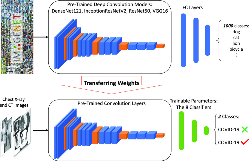
As shown in Fig. 1, the parameters of the convolutional layers are kept frozen during the training process. The convolutional layers of these five pretrained models are fed by X-ray and CT images for hierarchical feature extractions. The front end of the pretrained networks is then replaced by different machine learning classifiers to separate Covid and non-Covid cases. It is important to mention that we drop the pooling operation in the last convolutional layer of these pretrained networks. This is to avoid losing informative features before passing them to the classification models.

Fig. 1.

Block diagram of the proposed transfer learning-based framework for the COVID-19 detection using X-ray and CT images.

B. Uncertainty Quantification

Any classification study without reporting the predictive uncertainty estimates is not complete. There are two types of uncertainties, which needs to be considered for deep learning models [28]:

• 1)Aleatoric uncertainty which is related to the noise inherent in the data generating process. This type of uncertainty is irreducible.
• 2)Epistemic uncertainty which captures the ignorance about the model. In contrast to aleatoric uncertainty, epistemic uncertainty is reducible with collection of more training samples from diverse scenarios [9].

In this article, we mainly focus on epistemic uncertainty as it closely relates to the generalization power of models for new samples [29]–[31]. Here, we will use an ensemble of diverse models to obtain uncertainties associated with made inferences [29]. An ensemble consists of several models developed with different architectures, types, and sampled subsets. These model development differences cause diversity in the generalization power of models. Predictions obtained from individual models are then aggregated to obtain the final prediction. The prediction variance could be used for the calculation of the epistemic uncertainty [32].

Similar to work in [24] and [33], we calculate the prediction entropy as a measure of the epistemic uncertainty. The prediction entropy is a metric to measure the uncertainty in scores generated by different models [33]. The ensemble epistemic uncertainty is calculated as the entropy of the mean predictive distribution (by averaging all predicted distributions)

where is the set of parameters for the th network element and ranges over all classes. For instance, suppose that for a given input, an individual neural network predicts that the input belongs to class 1 with amount of probability and to class 0 with amount. If we repeat this procedure ten times for that specified input, it is similar to ensembling ten networks for predicting the output probability. The final output probability can be calculated using (1). Now, imagine the average probability predicts that an input belongs to class 1 and 0 with 0.6 and 0.4, respectively. Based on (2), the prediction entropy can be calculated as . It is obvious that the prediction entropy becomes zero when the output is assigned to a class with high probability and becomes maximum when the network is uncertain about its outcome.

III. Experiment Setup

A. Data Sets

There are two types of data sets used in this study: chest X-ray and breast CT scan. These two types of imagery data sets are the main sources of information that clinicians use for COVID-19 diagnosis. The description of these data sets is provided in this section. Also, statistical and machine learning classifiers applied to process features extracted by CNNs are briefly introduced.

1). Chest X-Ray Data Set:

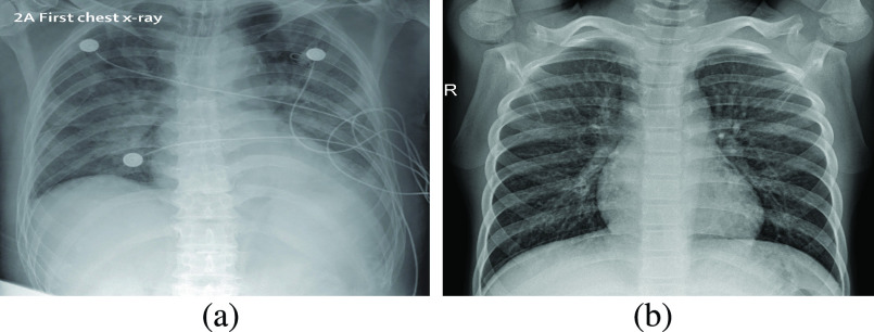
This data set is formed by taking 25 images of COVID-19 from [34] in the first step. We then add another 75 non-Covid cases of chest X-ray image from [35]. It is important to note that these non-Covid (normal) cases might consist of other unhealthy conditions, such as bacterial or viral infections, chronic obstructive pulmonary disease, and even a combination of two or more. Accordingly, what we mean by a normal or non-Covid case does not necessarily infer a healthy lower respiratory system. Two images of covid and normal classes are shown in Fig. 2. Fig. 2(b) shows a normal (non-Covid) case, yet virally infected. All images in this data set are accessible via this link: https://github.com/dara1400/Covid19-Xray-Dataset.

Fig. 2.

Two sample images from the X-ray data set. (a) Covid. (b) Normal.

2). CT Data Set:

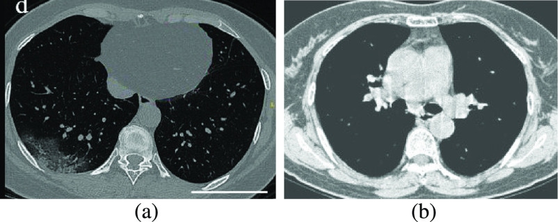
CT data set has 349 Covid images and 397 non-Covid images [36]. Health professionals prefer breast CT scans as they carry more information compared to chest X-rays to use for medical diagnosis. Fig. 3 shows both a Covid and a non-Covid case from the CT database.

Fig. 3.

Two sample images from the CT data set. (a) Covid. (b) Normal.

B. Pretrained Models

Here, we briefly introduce the four CNNs used in this study for extracting features.

1). VGG16 [25]:

This model is similar to AlexNet and consists of 13 convolution, nonlinear rectification, pooling, and three fully connected layers [25]. The filter size of the convolutional network is and the pooling size is . Due to its simple architecture, the VGG network is performed better than AlexNet.

2). ResNet50 [26]:

Residual convolutional network (ResNet) is one of the most popular deep structure, which is used for classification problem (winner of ImageNet competition in 2015). Residual blocks enable the network to provide a direct path to its early layers. This helps the gradient flow easily in the backpropagation algorithm.

3). DenseNet121 [37]:

DenseNet won the ImageNet competition in 2017. Traditional deep networks have only one connection between layers. However, in DenseNet, all layers receive all feature maps from previous layers as input [37]. This helps the network to decrease the number of parameters and also relieve the gradient vanishing.

4). InceptionResNetV2:

Szegedy et al. [27] presented a novel structure that helps to go deeper through convolution networks. Deep networks are prone to overfitting. They solve this solution using inception blocks. Furthermore, they use residual blocks and create InceptionResNetV2, which uses the combination of residual and inception blocks wisely.

High-level information about these pretrained models is shown in Table I. As shown in Fig. 1, network weights are kept frozen during the transfer learning procedure. The size of our input images is for VGG16, ResNet50, and DenseNet121. The input size for the InceptionResNetV2 architecture is .

TABLE I. Information About Four Considered Architectures for Transfer Learning.

Architecture	Paper	Year Proposed	Input Size	Number of Features	Number of Parameters
VGG16	2014	[25]		25,088	14,714,688
ResNet50	2015	[26]		100,352	23,587,712
DenseNet121	2017	[37]		50,176	7,037,504
InceptionResNetV2	2015	[27]		98,304	54,336,736

C. Classification Methods

The COVID-19 detection is a binary classification problem where the input is an image (chest X-ray or CT image) and the output is a binary label representing the presence or absence of COVID-19. Here, images are first processed by the convolutional layers of five pretrained networks. Hierarchically extracted features are then processed by multiple classifiers. We use eight classifiers to process features: k-nearest neighbors (kNNs), linear support vector machine (linear SVM), radial basis function (RBF) SVM, Gaussian process (GP), random forest (RF), multilayer perceptron (NN), Adaboost, and Naive Bayes. These classifiers are briefly introduced in the following.

1). k-Nearest Neighbor:

kNN is one of the simplest classification algorithms. It keeps a copy of all samples and classifies samples based on a similarity measure. This similarity measure is usually a kind of distance in the feature space. The most commonly used distance measures are Euclidean and Minkowski. In this article, we use and the Minkowski distance metric for the classification task. The Minkowski is calculated as

If , the Minkowski distance is the same as the Euclidean distance.

2). Support Vector Machine:

It is a practical solution for classification problem, especially in high dimensions. SVM uses line or hyperplane for dividing the data into appropriate classes. It tries to find a hyperplane with the largest distance to the most near data for each class (margin). The lower generalization error will be achieved when the margin becomes large [38].

3). RBF SVM:

It is a kind of SVM that uses the RBF kernel for calculating the similarity (distance) between two samples. RBF kernel for two typical samples ( ) can be calculated as follows:

4). Gaussian Process:

It is a set of random variables in a way that each set is described by a multivariate normal distribution. The final distribution of a GP is a joint distribution of all those random variables. GP uses covariance matrix and its inversion, and thus, it will be a lazy learning algorithm in high-dimensional space. It outputs a distribution that not only estimates the prediction but also provides prediction uncertainty estimates. We use RBF kernel with a length scale equal to one for GP classifiers in this study.

5). Neural Network:

A feedforward NN finds a nonlinear mapping between the fixed-size inputs and the output (target). The network is composed of several hidden layers and processing units called neurons. A neuron receives inputs from neurons of the previous layer and generates its own output based on the assigned activation function. The connection weights between layers of the network are trained using training algorithms, such as stochastic gradient descent or adaptive moment estimation (Adam).

6). Random Forest:

RF classifier includes several decision trees developed in parallel. These trees are developed by randomly selecting a subset of features and samples from the original training samples. Each tree will vote and the class that has the most votes will be the final prediction. In this article, we set the number of decision trees to 10.

7). Adaboost:

Adaboost forms an efficient classifier by mixing several weak classifiers. Classifiers are formed in a serial approach in contrast to RF where classifiers are formed in parallel. Each classifier focuses on fixing mistakes made by previous classifiers. We here set the number of weak classifiers to 50.

8). Naive Bayes:

Naive Bayes classifiers are the simplest Bayesian networks that use the Bayes theorem. We use the Gaussian naive Bayes that predict a posterior using a normal prior based on the Bayes theory.

Full information about these classifiers could be found in basic machine learning and statistical books [39]–[42].

IV. Simulations and Results

The simulation results and discussions are provided in this section. We first present the results obtained by different classifiers processing features extracted by pretrained CNNs. We then focus on the uncertainty quantification problem using NN models and discuss its importance for the diagnosis of COVID-19.

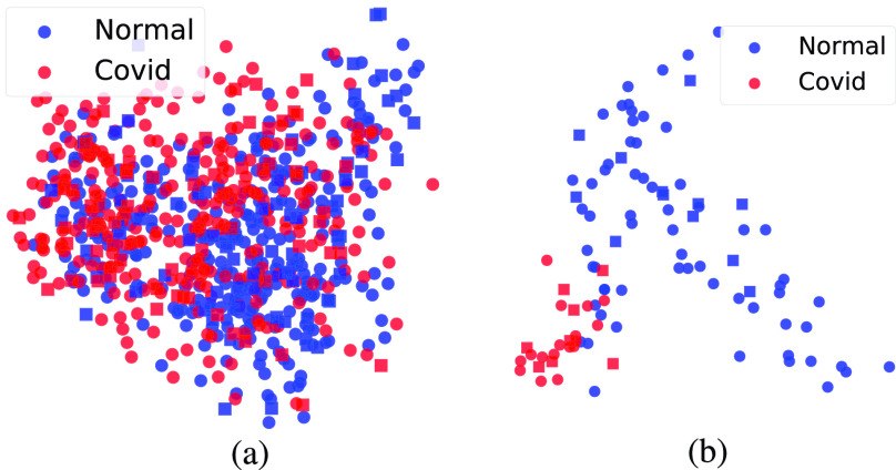
To build an intuition about samples, we first extract deep features using the method shown in Fig. 1 and then map them to the 2-D space using the principal component analysis (PCA) algorithm. Fig. 4 shows VGG16 features in the 2-D space. As reported in Table I, the total number of extracted features for VGG16 is 25 088. Obviously, the number of samples for CT data set is much higher and it is more balanced than the X-ray data set. Also, it is interesting to see that normal (non-Covid) and Covid cases are fairly distinguishable for X-ray images in 2-D space. In contrast, the decision boundary cannot be reasonably drawn in two dimensions for CT images.

Fig. 4.

2-D representation of X-ray and CT images processed by VGG16 and PCA. (a) CT. (b) X-ray.

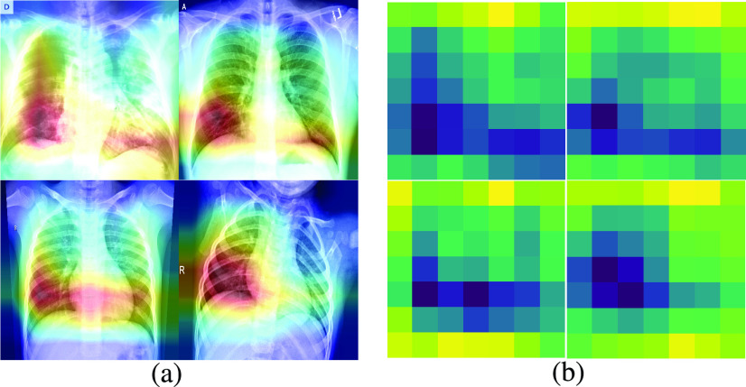
To show the effectiveness of extracted features, we go through the concept of Grad-CAM. Neural network architecture is usually called as black box since it needs some inputs and produces some outputs in a way that one has not any idea about how it works. In this regard, Selvaraju et al. [43] proposed a method in which the most effective pixels that lead to final prediction can be found. Gradient-weighted class activation mapping (Grad-CAM) gives us some visual explanations (spatial information masked by layers) of how our model makes a decision. This can be estimated by finding the gradients of the target backpropagating through the convolutional layers producing a heatmap. This heatmap will highlight the most prominent regions of input for the classification decision.

To gain an insight into our proposed model, we apply the same structure, which can find the most important pixels of a typical image to predict a specific label. Fig. 5 shows the Grad-CAMs and heatmaps of four images, giving us an explanation of how our VGG16 is working.

Fig. 5.

Grad-CAMs and Heatmaps show how our model makes decision. (a) Grad-CAMs. (b) Heatmaps.

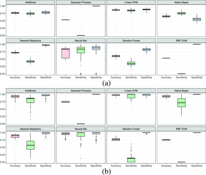
Accuracy, sensitivity, and specificity are considered for the model evaluation. Purely relying on accuracy could lead to misleading results as both data sets and in particular X-ray one are imbalanced. For obtaining statistically valid conclusions, we train every single classifier 100 times using obtained features from pretrained CNNs. For each run, the performance metrics are calculated, and then, the box plot graph is generated. Fig. 6 shows the box plots for CT and X-ray data sets, respectively, for accuracy, sensitivity, and specificity. It is noted that those values are calculated without PCA for all classifiers trained 100 times (all features passed to classifiers).

Fig. 6.

Distribution of accuracy, sensitivity, and specificity associated with (a) CT and (b) X-ray data sets, respectively (the top results are for CT data set of our different classifiers).

It is observed that the more the number of features, the less the ability of RBF SVM and GP to correctly classify samples. This is because they use the covariance matrix and its inversion, which in turn drops the sensitivity value to zero, making them unreliable. In contrast, linear SVM and NN prove to be the best ones among considered classifiers. This is because they use simple hyperplanes to separate features of two classes.

ROC curves for all pretrained CNNs and classifiers are shown in Fig. 7 for a typical run. As expected, linear SVM and NN models have the highest AUC values among all classifiers. An important observation is that the performance of classifiers significantly varies based on hierarchically extracted features by convolutional layers of four pretrained CNNs.

Fig. 7.

ROC-AUC plots are shown for CT images using four architectures (VGG16, InceptionResNetV2, ResNet50, and DenseNet121) and eight classifiers. As can be seen, linear SVM and NN (MLP) are the bests and their AUC values are greater than others. Also, it is noted that the performance of classifiers closely depends on the quality of features extracted by the convolutional layers of four considered architectures. (a) VGG16. (b) InceptionResNetV2. (c) ResNet50. (d) DenseNet121.

To comprehensively compare different architectures for feature extraction, we train and evaluate each classifier 100 times. Then, we average all predictions to obtain a reliable estimate of the sample label. Then, performance metrics, including accuracy, sensitivity, specificity, and AUC value, are calculated. Tables II and III report these performance metrics for CT and X-ray data sets. Reported values are given in percent. Having compared all models, we find that no model outperforms others for most cases than others. Linear SVM also achieves the best results for each model.

TABLE II. Performance Comparison of Four Architectures and Eight Classifiers (32 Combinations) for CT Images. All Values are Given in Percent.

Model	Classifier	Accuracy	Sensitivity	Specificity	AUC
DenseNet121	AdaBoost	78.9 ± 7.6	76.5 ± 11.5	80.1 ± 8.4	81.9 ± 5.8
	Gaussian Process	53.1 ± 10.9	0.0	1.0	0.5 ± 0.9
	Linear SVM	85.9 ± 5.9	84.9 ± 8.4	86.8 ± 6.3	93.1 ± 3.4
	Naive Bayes	74.9 ± 5.5	72.4 ± 24.4	77 ± 11.5	77 ± 9.1
	Nearest Neighbors	79.8 ± 6	69.7 ± 13.5	88.8 ± 5.3	86.8 ± 5.4
	Neural Net	83.4 ± 14.4	82 ± 28	84.6 ± 24	92.7 ± 13.4
	RBF SVM	53.1 ± 2.3	0.0	1.0	57 ± 3.1
	Random Forest	62.3 ± 9.2	46.2 ± 17.7	76.3 ± 11.7	67.4 ± 10.3
InceptionResNetV2	AdaBoost	75.2 ± 8.3	72.6 ± 12.8	77.5 ± 9.7	82.7 ± 7.4
	Gaussian Process	53.1 ± 10.9	0.0	1.0	0.5 ± 0.4
	Linear SVM	84.3 ± 7.3	83.2 ± 9	91.9 ± 7.4	91.9 ± 4.1
	Naive Bayes	75.7 ± 2.5	76.6 ± 3.8	75 ± 12.8	77.3 ± 13.6
	Nearest Neighbors	75.8 ± 8.2	57.3 ± 14.9	92 ± 4.4	84.4 ± 6.8
	Neural Net	80.7 ± 16.5	79.4 ± 28.1	82.6 ± 29	87.8 ± 15.6
	RBF SVM	53.1 ± 11	0.0	1.0	55 ± 2.4
	Random Forest	59.1 ± 9.9	42.3 ± 18	73.4 ± 13	68.7 ± 11.6
ResNet50	AdaBoost	76.1 ± 9.4	73.9 ± 13.5	78 ± 9.8	83.9 ± 7.6
	Gaussian Process	53.1 ± 11	0.0	1.0	0.5 ± 0.4
	Linear SVM	87.9 ± 5.8	86.5 ± 7.1	89.1 ± 5.4	94.2 ± 2.9
	Naive Bayes	59.5 ± 9.8	70.1 ± 30.6	50 ± 25.4	60.1 ± 5.5
	Nearest Neighbors	78.9 ± 8.2	65.2 ± 14.4	91.1 ± 4.8	87.2 ± 6.4
	Neural Net	84.6 ± 16.4	83.1 ± 30.4	88.3 ± 27.9	91.7 ± 16.7
	RBF SVM	53.1 ± 11	0.0	1.0	51 ± 0.8
	Random Forest	59.3 ± 9.1	35.1 ± 16.4	80.6 ± 10.1	63.3 ± 11.4
VGG16	AdaBoost	76.8 ± 7.8	73.9 ± 13.1	79.2 ± 8.9	84.2 ± 7.1
	Gaussian Process	53.1 ± 11	0.0	1.0	0.5 ± 0.4
	Linear SVM	86.5 ± 5.8	84.8 ± 8.2	88.1 ± 5.9	93.3 ± 3.3
	Naive Bayes	64.2 ± 12.2	74.5 ± 18.9	55 ± 22.5	64.8 ± 8.9
	Nearest Neighbors	71.4 ± 6.9	42.3 ± 14	97.1 ± 2.5	83.8 ± 6.2
	Neural Net	84.6 ± 16.3	85.8 ± 32.1	87.6 ± 27	92.8 ± 18.6
	RBF SVM	53.1 ± 11	0.0	1.0	0.5 ± 0.4
	Random Forest	59.7 ± 9	34.4 ± 16.4	82 ± 9.5	64.2 ± 11.8

TABLE III. Performance Comparison of Four Architectures and Eight Classifiers (32 Combinations) for X-Ray Images. All Values are Given in Percent.

Model	Classifier	Accuracy	Sensitivity	Specificity	AUC
DenseNet121	AdaBoost	91 ± 5.9	77.7 ± 15.8	95.4 ± 5.2	96.6 ± 3.9
	Gaussian Process	74.8 ± 1.7	0.0	1.0	51 ± 0.8
	Linear SVM	96.4 ± 3.1	93.9 ± 9.3	97.2 ± 3.7	99.5 ± 0.8
	Naive Bayes	82.3 ± 5	31.6 ± 18.5	99.4 ± 0.5	65.5 ± 9.2
	Nearest Neighbors	89.4 ± 4.6	64.1 ± 18.1	97.8 ± 2.9	95.4 ± 4.2
	Neural Net	93.2 ± 5.7	80.7 ± 24.1	97.4 ± 2.9	98.9 ± 1.2
	RBF SVM	75 ± 1.7	0.0	1.0	51 ± 1.1
	Random Forest	78.9 ± 4.3	20 ± 15.5	98.5 ± 2.6	82.3 ± 9.3
InceptionResNetV2	AdaBoost	89.5 ± 5.6	73.8 ± 17.8	94.8 ± 5.2	94.9 ± 5.4
	Gaussian Process	74.8 ± 1.7	0.0	1.0	51 ± 1.1
	Linear SVM	98 ± 3.2	96.3 ± 7.8	98.5 ± 3.5	99.8 ± 0.6
	Naive Bayes	75.3 ± 2	1.1	1.0	50.5 ± 1.8
	Nearest Neighbors	89.9 ± 5.4	62.2 ± 20.3	99.3 ± 2.3	96 ± 4.7
	Neural Net	89.9 ± 12.6	72.7 ± 24.6	95.6 ± 17.1	97.5 ± 8.5
	RBF SVM	75.1 ± 1.7	0.0	1.0	51 ± 1.1
	Random Forest	77.6 ± 4.3	13.9 ± 13.8	98.9 ± 2.1	80.6 ± 9.7
ResNet50	AdaBoost	92.6 ± 6.1	84.4 ± 17.1	95.3 ± 5.5	97.6 ± 4.1
	Gaussian Process	75.1 ± 1.6	0.0	1.0	51 ± 1.1
	Linear SVM	98.6 ± 2.1	99.9 ± 1.2	98.2 ± 2.8	99.7 ± 0.6
	Naive Bayes	77.8 ± 3.9	12.5 ± 12.5	1.0	56.3 ± 6.7
	Nearest Neighbors	94 ± 4.4	78.4 ± 17.7	99.2 ± 2.6	97.7 ± 4.9
	Neural Net	92.5 ± 6.4	85.5 ± 24.1	94.8 ± 7.3	98 ± 3.2
	RBF SVM	75 ± 1.7	0.0	1.0	51 ± 1.1
	Random Forest	76.3 ± 3.3	80 ± 10.8	99.1 ± 2	80.8 ± 9.6
VGG16	AdaBoost	89.9 ± 5.5	85.9 ± 17.9	94.9 ± 4.8	94.1 ± 6.8
	Gaussian Process	74.1 ± 1.7	0.0	1.0	51 ± 1
	Linear SVM	96.6 ± 3.4	98.8 ± 9.9	98.3 ± 3.1	99.6 ± 0.7
	Naive Bayes	90.2 ± 5.1	70.8 ± 20.3	99.3 ± 1.6	75 ± 10
	Nearest Neighbors	89.3 ± 4.5	57.3 ± 7	98.9 ± 3	83.9 ± 8.3
	Neural Net	94.3 ± 6.1	98.8 ± 25.3	97.5 ± 5.7	98.3 ± 2.1
	RBF SVM	76.1 ± 1.7	0.0	1.0	51 ± 1
	Random Forest	76.5 ± 3.1	13.2 ± 10.2	99.5 ± 1.6	82.8 ± 9.3

Comparing the designed network to that of [36], our transfer learning-based method outperforms theirs. The best results are achieved using ResNet50 and linear SVM classifier (an accuracy of 87.9%). This is more than 3% better than the best results reported in [36]. (84.7% accuracy). This improvement is mainly due to a better hierarchical extraction of features using ResNet50 and an optimal selection of the classifier (linear SVM).

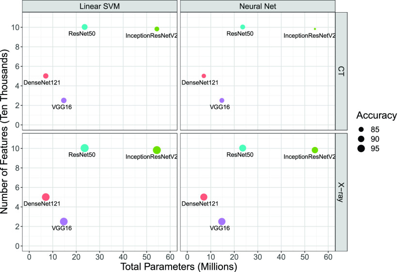
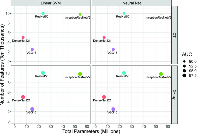
It is also important to consider the network size and the number of deep features when comparing the performance of pretrained CNNs for COVID-19 detection. Figs. 8 and 9 show the average of the classification performance (accuracy and AUC) for linear SVM and NN models in the 2-D space formed by the number of CNN parameters (millions) and the number of features (ten thousands), respectively. The size of each point represents the accuracy and AUC metrics of the trained classifiers using features extracted by pretrained CNNs. The bigger the point, the better the performance. We generate these charts only for linear SVM and NN models as they are the best performing ones according to results presented in Tables II and III. According to Figs. 8 and 9, VGG16 is the most efficient pretrained CNNs for COVID-19 detection. It has the least number of parameters and extracts the smallest number of features. Those features are the most informative and discriminative ones as both linear and NN models achieve the best results using them. In contrast, the massive network of InceptionResNetV2 offers the most number of features that have the least information content among the investigated network. Another key observation is the choice of the pretrained CNN that has a direct and profound impact on the overall performance of the COVID-19 classification model. Last but not least, one may conclude that bigger networks, such as ResNet50 and InceptionResNetV2, do not necessarily extract more informative and discriminative features.

Fig. 8.

Accuracy average in the 2-D space of the number of CNN parameters (millions) and the number of features (ten thousands). The size of each point is an indication of the classifier accuracy (mean value in 100 runs).

Fig. 9.

AUC average in the 2-D space of the number of CNN parameters (millions) and the number of features (ten thousands). The size of each point is an indication of the AUC metric (mean value in 100 runs).

It is also quite important to quantify uncertainties associated with predictions. Here, we generate predictive uncertainty estimates for NN models. As mentioned before, there are several ways of generating ensemble networks. We use the entire data set in the training step because the availability of more samples improves the generalization power of NN models. Twenty individual NN models with different architectures are first trained to form an ensemble. NN models have a hidden layer and their number of hidden neurons is randomly selected between 50 and 400.

Fig. 10 shows the predictive uncertainty estimates for both Covid and non-Covid cases in a 2-D space. Fig. 10(a)–(d) shows epistemic uncertainties for the X-ray data set. Fig. 10(e)–(h) shows epistemic uncertainties for the CT data set. The 2-D space is obtained after applying PCA to reduce the dimensionality of obtained features from pretrained CNNs. This projection to the 2-D space is done to ensure that samples could be visualized against the calculated predictive uncertainty estimates. The darker the color of filled area, the higher the uncertainty level. According to Fig. 10(a)–(d), the level of epistemic uncertainty for the X-ray data set is fairly low. While the projected features in the 2-D space are in different locations for four pretrained CNNs, the NN classifiers generate very similar results. This consistency leads to a low uncertainty. In contrast, the predictive uncertainty estimates for CT images are quite high. This is evident from the large dark area in Fig. 10(e)–(h). These indicate that individual NN models in the ensemble have a different generalization power and produce significantly inconsistent results. There is no perfect agreement between all models about the predictive labels of these samples. Accordingly, more care should be exercised when using machine learning predictions for COVID-19 diagnosis using CT images.

Fig. 10.

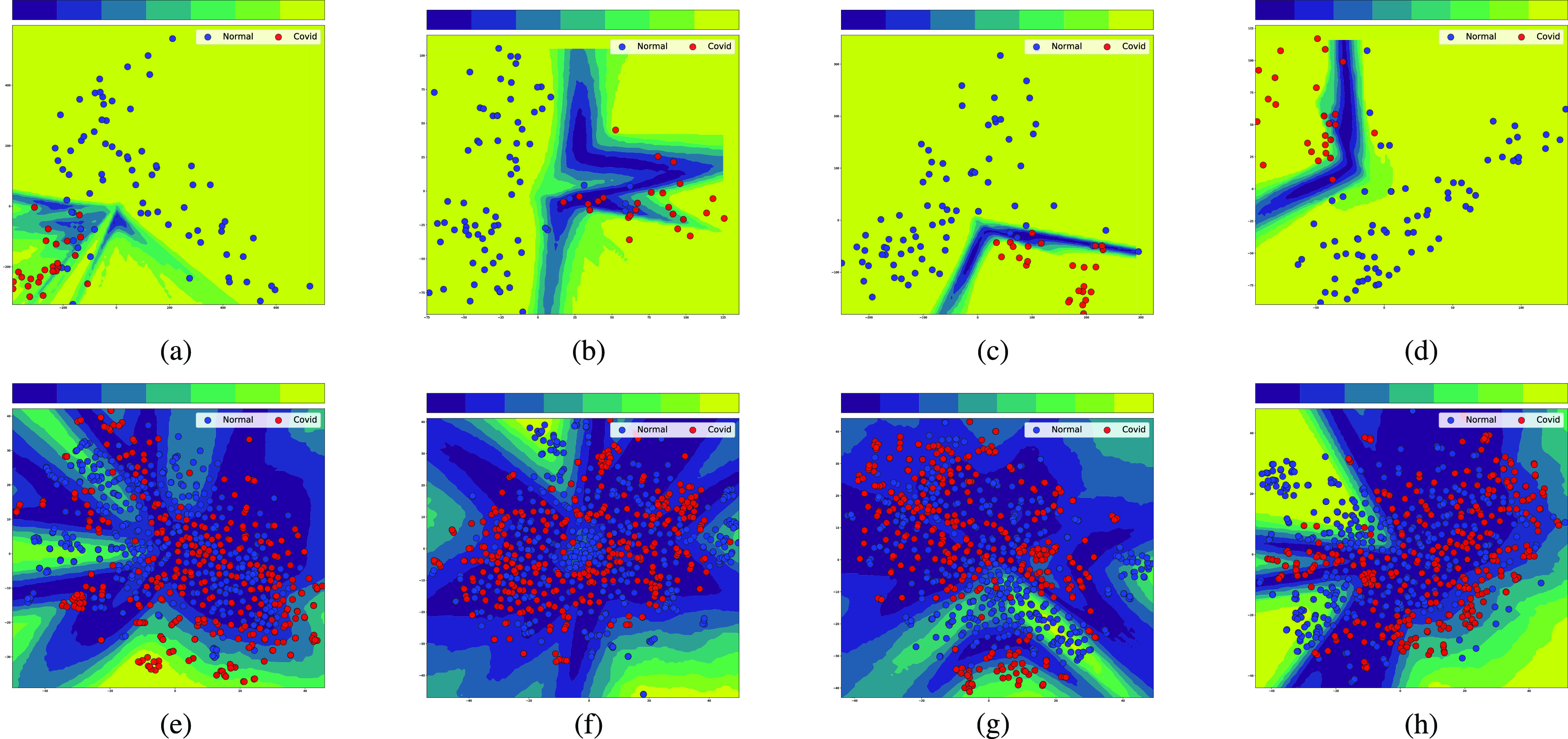
Uncertainty quantification using 20 individual neural networks working as an ensemble. They differ in the number of neurons in their hidden layer before applying a multilayer perceptron classifier. The darker the color, the higher the uncertainty level. Samples on dark parts of the plot have a high level of predictive uncertainty as the 20 models could not all agree on the predicted label. (a) VGG16. (b) InceptionResNetV2. (c) ResNet50. (d) DenseNet121. (e) VGG16. (f) InceptionResNetV2. (g) ResNet50. (h) DenseNet121.

V. Conclusion

The purpose of this study was to investigate the suitability of deep transfer learning for COVID-19 diagnosis using medical imaging. The key motivation was the lack of access to large repositories of images for developing deep neural networks from scratch. Leveraging the transfer learning framework, we apply four pretrained deep CNNs (VGG16, ResNet50, DenseNet121, and InceptionResNetV2) to hierarchically extract informative and discriminative features from chest X-ray and CT images. The parameters of the convolutional layers are kept frozen during the training process. Extracted features are then processed by multiple classification techniques. Obtained results indicate that linear SVM and multilayer perceptron outperforms other methods in terms of the medical diagnosis accuracy for both X-ray and CT images. It is also observed that better prediction results and medical diagnosis could be achieved using CT images as they are much richer in information compared to X-ray images.

There are many rooms for improvement and further exploration. The performance of transfer learning algorithms could be majorly improved by fine-tuning them to extract more informative and discriminative features. Features obtained from different transfer learning models could be combined to develop hybrid models. Also, predictions from individual models could be combined to form ensembles. Last but not least, a state-of-the-art method could be applied for more comprehensive estimation of the uncertainty measures.

Biographies

Afshar Shamsi received the B.Sc. degree in electrical engineering and the M.Sc. degree in control engineering from Tabriz University, Tabriz, Iran, in 2009 and 2013, respectively.

He is currently working as an Electrical Engineer with the ASR Group, Tehran, Iran. His main interests include machine learning and uncertainty quantification techniques.

Hamzeh Asgharnezhad received the B.Sc. degree in electrical engineering from Tabriz University, Tabriz, Iran, in 2009, and the Master of Business Administration from Nooretouba University, Tehran, Iran, in 2012.

He has been studying, researching, and working in the field of artificial intelligence since 2018. His current focus is on uncertainty quantification in machine learning.

Shirin Shamsi Jokandan received the D.Pharm. degree from RGUHS University, Bengaluru, India, in 2017.

She did a one-year internship at Baptist Hospital, Bengaluru. She now works as a community pharmacist in Iran.

Abbas Khosravi (Senior Member, IEEE) received the B.Sc. degree in electrical engineering from the Sharif University of Technology, Tehran, Iran, in 2002, the M.Sc. degree in electrical engineering from the Amirkabir University of Technology, Tehran, in 2005, and the Ph.D. degree from Deakin University, Geelong, VIC, Australia, in 2010.

He is currently an Associate Professor with the Institute for Intelligent systems Research and Innovation (IISRI), Deakin University. His research interests include artificial intelligence, data mining, and optimization.

Parham M. Kebria (Member, IEEE) received the B.Sc. and M.Sc. degrees in electrical engineering, in 2011 and 2014, respectively, and the Ph.D. degree in information technology from Deakin University, Waurn Ponds, VIC, Australia, in 2019. He is currently a Postdoctoral Research Fellow with the Institute for Intelligent Systems Research and Innovation (IISRI), Deakin University. His research interests include, but not limited to, robotics and artificial intelligence mainly with medical applications.

Darius Nahavandi (Member, IEEE) received the Bachelor of Health Science and Ph.D. degrees from Deakin University, Geelong, VIC, Australia, in 2015 and 2018, respectively.

He is currently a Research Fellow with the Institute of Intelligent Systems Research and Innovation, Deakin University. Throughout the years, he has contributed to a range of projects involving the automotive, mining, and defense industries with a primary focus on innovation for human factors. His research consists of investigating human performance factors using advanced technologies both in the lab environment and industry settings.

Saeid Nahavandi (Fellow, IEEE) received the Ph.D. degree from Durham University, Durham, U.K., in 1991.

He is currently an Alfred Deakin Professor, a Pro Vice-Chancellor, the Chair of Engineering, and the Founding Director of the Institute for Intelligent Systems Research and Innovation at Deakin University, Geelong, VIC, Australia. His research interests include modeling of complex systems, robotics, and haptics. He has published over 900 scientific papers in various international journals and conferences.

Dr. Nahavandi is a fellow of Engineers Australia (IEAust), the Institution of Engineering and Technology (IET), and the Australian Academy of Technology and Engineering (ATSE). He is the Editor-in-Chief of IEEE SMC Magazine, a Senior Associate Editor of the IEEE Systems Journal, an Associate Editor of the IEEE Transactions on Systems, Man and Cybernetics: Systems, and an IEEE Press Editorial Board Member.

Dipti Srinivasan (Fellow, IEEE) received the M.Eng. and Ph.D. degrees in electrical engineering from the National University of Singapore, Singapore, in 1991 and 1994, respectively.

She worked as a Post-Doctoral Researcher with the University of California at Berkeley, Berkeley, CA, USA, from 1994 to 1995, before joining the National University of Singapore, Singapore, where she is currently a Professor with the Department of Electrical and Computer Engineering. Her research interest is in the application of soft computing techniques to engineering optimization and control problems.

Dr. Srinivasan is serving as an Associate Editor for the IEEE Transactions on Neural Networks and Learning Systems, the IEEE Transactions on Evolutionary Computation, the IEEE Transactions on Sustainable Energy, and IEEE Computational Intelligence Magazine.

Funding Statement

This work was supported by the Australian Research Council Discovery Projects funding scheme (project DP190102181 and DP210101465).

References

- [1].(2020). Coronavirus Disease 2019 (COVID-19). Accessed: Feb. 27, 2020. [Online]. Available: https://www.who.int/emergencies/diseases/novel-coronavirus-2019/situati%on-reports
- [2].Emergency Approval to Use Diagnostic Test for Corona-Virus. Accessed: Jan. 23, 2020. [Online]. Available: https://www.reuters.com/article/us-china-health-cdc/u-s-cdc-seeks-emergency-%approval-to-use-diagnostic-test-for-coronavirus-idUSKBN1ZM2XS
- [3].Bogoch I. I., Watts A., Thomas-Bachli A., Huber C., Kraemer M. U. G., and Khan K., “Pneumonia of unknown aetiology in wuhan, China: Potential for international spread via commercial air travel,” J. Travel Med., vol. 27, no. 2, Mar. 2020. [DOI] [PMC free article] [PubMed] [Google Scholar]
- [4].Huang C.et al. , “Clinical features of patients infected with 2019 novel coronavirus in Wuhan, China,” Lancet, vol. 395, pp. 497–506, May 2020. [DOI] [PMC free article] [PubMed] [Google Scholar]
- [5].Alizadehsani R.et al. , “Machine learning-based coronary artery disease diagnosis: A comprehensive review,” Comput. Biol. Med., vol. 111, Aug. 2019, Art. no. 103346. [DOI] [PubMed] [Google Scholar]
- [6].Janowczyk A. and Madabhushi A., “Deep learning for digital pathology image analysis: A comprehensive tutorial with selected use cases,” J. Pathol. Informat., vol. 7, no. 1, p. 29, 2016. [DOI] [PMC free article] [PubMed] [Google Scholar]
- [7].Hassanpour S.et al. , “Deep learning for classification of colorectal polyps on whole-slide images,” J. Pathol. Informat., vol. 8, no. 1, p. 30, 2017. [DOI] [PMC free article] [PubMed] [Google Scholar]
- [8].Vununu C., Lee S.-H., and Kwon K.-R., “A deep feature extraction method for HEp-2 cell image classification,” Electronics, vol. 8, no. 1, p. 20, Dec. 2018. [Google Scholar]
- [9].Alizadehsani R.et al. , “Model uncertainty quantification for diagnosis of each main coronary artery stenosis,” Soft Comput., vol. 24, no. 13, pp. 10149–10160, Jul. 2020. [Google Scholar]
- [10].Jaiswal A. K., Tiwari P., Kumar S., Gupta D., Khanna A., and Rodrigues J. J. P. C., “Identifying pneumonia in chest X-rays: A deep learning approach,” Measurement, vol. 145, pp. 511–518, Oct. 2019. [Google Scholar]
- [11].Rajpurkar P.et al. , “CheXNet: Radiologist-level pneumonia detection on chest X-Rays with deep learning,” 2017, arXiv:1711.05225. [Online]. Available: http://arxiv.org/abs/1711.05225 [Google Scholar]
- [12].Ozturk T., Talo M., Yildirim E. A., Baloglu U. B., Yildirim O., and Rajendra Acharya U., “Automated detection of COVID-19 cases using deep neural networks with X-ray images,” Comput. Biol. Med., vol. 121, Jun. 2020, Art. no. 103792. [DOI] [PMC free article] [PubMed] [Google Scholar]
- [13].Apostolopoulos I. D. and Bessiana T., “COVID-19: Automatic detection from X-ray images utilizing transfer learning with convolutional neural networks,” 2020, arXiv:2003.11617. [Online]. Available: http://arxiv.org/abs/2003.11617 [DOI] [PMC free article] [PubMed] [Google Scholar]
- [14].Narin A., Kaya C., and Pamuk Z., “Automatic detection of coronavirus disease (COVID-19) using X-ray images and deep convolutional neural networks,” 2020, arXiv:2003.10849. [Online]. Available: http://arxiv.org/abs/2003.10849 [DOI] [PMC free article] [PubMed] [Google Scholar]
- [15].Song Y.et al. , “Deep learning enables accurate diagnosis of novel coronavirus (COVID-19) with ct images,” Medrxiv, Jan. 2020. [DOI] [PMC free article] [PubMed]
- [16].Barstugan M., Ozkaya U., and Ozturk S., “Coronavirus (COVID-19) classification using CT images by machine learning methods,” 2020, arXiv:2003.09424. [Online]. Available: http://arxiv.org/abs/2003.09424 [Google Scholar]
- [17].Zheng C.et al. , “Deep learning-based detection for COVID-19 from chest ct using weak label,” Medrxiv, Jan. 2020.
- [18].Xu X.et al. , “Deep learning system to screen coronavirus disease 2019 pneumonia,” 2020, arXiv:2002.09334. [Online]. Available: http://arxiv.org/abs/2002.09334 [Google Scholar]
- [19].Postels J., Ferroni F., Coskun H., Navab N., and Tombari F., “Sampling-free epistemic uncertainty estimation using approximated variance propagation,” 2019, arXiv:1908.00598. [Online]. Available: http://arxiv.org/abs/1908.00598 [Google Scholar]
- [20].Hendrycks D. and Gimpel K., “A baseline for detecting misclassified and Out-of-Distribution examples in neural networks,” 2016, arXiv:1610.02136. [Online]. Available: http://arxiv.org/abs/1610.02136 [Google Scholar]
- [21].Zhe Liu J., Lin Z., Padhy S., Tran D., Bedrax-Weiss T., and Lakshminarayanan B., “Simple and principled uncertainty estimation with deterministic deep learning via distance awareness,” 2020, arXiv:2006.10108. [Online]. Available: http://arxiv.org/abs/2006.10108 [Google Scholar]
- [22].Amodei D., Olah C., Steinhardt J., Christiano P., Schulman J., and Mané D., “Concrete problems in AI safety,” 2016, arXiv:1606.06565. [Online]. Available: http://arxiv.org/abs/1606.06565 [Google Scholar]
- [23].Ghoshal B. and Tucker A., “Estimating uncertainty and interpretability in deep learning for coronavirus (COVID-19) detection,” 2020, arXiv:2003.10769. [Online]. Available: http://arxiv.org/abs/2003.10769 [Google Scholar]
- [24].van Amersfoort J., Smith L., Whye Teh Y., and Gal Y., “Simple and scalable epistemic uncertainty estimation using a single deep deterministic neural network,” Mar. 2020, arXiv:2003.02037. [Online]. Available: https://arxiv.org/abs/2003.02037 [Google Scholar]
- [25].Simonyan K. and Zisserman A., “Very deep convolutional networks for large-scale image recognition,” 2014, arXiv:1409.1556. [Online]. Available: http://arxiv.org/abs/1409.1556 [Google Scholar]
- [26].He K., Zhang X., Ren S., and Sun J., “Deep residual learning for image recognition,” 2015, arXiv:1512.03385. [Online]. Available: http://arxiv.org/abs/1512.03385 [Google Scholar]
- [27].Szegedy C.et al. , “Going deeper with convolutions,” in Proc. IEEE Conf. Comput. Vis. Pattern Recognit. (CVPR), Jun. 2015, pp. 1–9. [Google Scholar]
- [28].Kendall A. and Gal Y., “What uncertainties do we need in Bayesian deep learning for computer vision?” in Advances in Neural Information Processing Systems, Guyon I., Luxburg U. V., Bengio S., Wallach H., Fergus R., Vishwanathan S., and Garnett R., Eds. Red Hook, NY, USA: Curran Associates, 2017, pp. 5574–5584. [Google Scholar]
- [29].Lakshminarayanan B., Pritzel A., and Blundell C., “Simple and scalable predictive uncertainty estimation using deep ensembles,” 2016, arXiv:1612.01474. [Online]. Available: http://arxiv.org/abs/1612.01474 [Google Scholar]
- [30].Kabir H. M. D., Khosravi A., Hosen M. A., and Nahavandi S., “Neural network-based uncertainty quantification: A survey of methodologies and applications,” IEEE Access, vol. 6, pp. 36218–36234, 2018. [Google Scholar]
- [31].Quan H., Khosravi A., Yang D., and Srinivasan D., “A survey of computational intelligence techniques for wind power uncertainty quantification in smart grids,” IEEE Trans. Neural Netw. Learn. Syst., vol. 31, no. 11, pp. 4582–4599, Nov. 2020. [DOI] [PubMed] [Google Scholar]
- [32].Hosen M. A., Khosravi A., Nahavandi S., and Creighton D., “Improving the quality of prediction intervals through optimal aggregation,” IEEE Trans. Ind. Electron., vol. 62, no. 7, pp. 4420–4429, Jul. 2015. [Google Scholar]
- [33].Gal Y., Uncertainty in Deep Learning, vol. 1. Cambridge, U.K.: Cambridge Univ. Press, 2016, p. 3. [Google Scholar]
- [34].Paul Cohen J., Morrison P., and Dao L., “COVID-19 image data collection,” 2020, arXiv:2003.11597. [Online]. Available: http://arxiv.org/abs/2003.11597 [Google Scholar]
- [35].(2020). Chest X-ray Images (Pneumonia). Accessed: Feb. 17, 2020. [Online]. Available: https://www.kaggle.com/paultimo/thymooney/chest-xray-pneumonia
- [36].Yang X., He X., Zhao J., Zhang Y., Zhang S., and Xie P., “COVID-CT-dataset: A CT scan dataset about COVID-19,” 2020, arXiv:2003.13865. [Online]. Available: http://arxiv.org/abs/2003.13865 [Google Scholar]
- [37].Huang G., Liu Z., Van Der Maaten L., and Weinberger K. Q., “Densely connected convolutional networks,” in Proc. IEEE Conf. Comput. Vis. Pattern Recognit. (CVPR), Jul. 2017, pp. 4700–4708. [Google Scholar]
- [38].Friedman J., Hastie T., and Tibshirani R., The Elements of Statistical Learning, vol. 1. New York, NY, USA: Springer, 2001. [Google Scholar]
- [39].James G., Witten D., Hastie T., and Tibshirani R., An Introduction to Statistical Learning, vol. 112. New York, NY, USA: Springer, 2013. [Google Scholar]
- [40].Bishop C. M., Pattern Recognition and Machine Learning. New York, NY, USA: Springer, 2006. [Google Scholar]
- [41].Hastie T., Tibshirani R., and Friedman J., The Elements of Statistical Learning: Data Mining, Inference, and Prediction. New York, NY, USA: Springer, 2009. [Google Scholar]
- [42].Murphy K. P., Mach. learning: A Probabilistic Perspective. Cambridge, MA, USA: MIT Press, 2012. [Google Scholar]
- [43].Selvaraju R. R., Cogswell M., Das A., Vedantam R., Parikh D., and Batra D., “Grad-CAM: Visual explanations from deep networks via gradient-based localization,” in Proc. IEEE Int. Conf. Comput. Vis. (ICCV), Oct. 2017, pp. 618–626. [Google Scholar]