Augmented Multicenter Graph Convolutional Network for COVID-19 Diagnosis

Abstract

Chest computed tomography (CT) scans of coronavirus 2019 (COVID-19) disease usually come from multiple datasets gathered from different medical centers, and these images are sampled using different acquisition protocols. While integrating multicenter datasets increases sample size, it suffers from inter-center heterogeneity. To address this issue, we propose an augmented multicenter graph convolutional network (AM-GCN) to diagnose COVID-19 with steps as follows. First, we use a 3-D convolutional neural network to extract features from the initial CT scans, where a ghost module and a multitask framework are integrated to improve the network's performance. Second, we exploit the extracted features to construct a multicenter graph, which considers the intercenter heterogeneity and the disease status of training samples. Third, we propose an augmentation mechanism to augment training samples which forms an augmented multicenter graph. Finally, the diagnosis results are obtained by inputting the augmented multi-center graph into GCN. Based on 2223 COVID-19 subjects and 2221 normal controls from seven medical centers, our method has achieved a mean accuracy of 97.76%. The code for our model is made publicly.¹

I. Introduction

Since the first report of coronavirus disease 2019 (COVID-19) in China, the disease has spread rapidly to the whole world, which has caused over 26 million cases with a total of 0.86 million deaths by September 6, 2020. As the sensitivity of the widely used real-time reverse transcription-polymerase chain reaction is only about 60–70%, the chest computed tomography (CT) is vital for the early diagnosis of this disease [1], exhibiting good sensitivity and speed [2]. The CT images of COVID-19 patients and healthy people are shown in Fig. 1. It is highly desirable to automate COVID-19 diagnosis to relieve the burden on radiologists and physicians.

Fig. 1.

CT images of severe case (left), mild case (middle), and healthy case (right).

In existing work for automatic COVID-19 diagnosis, many focus in applying or improving current neutral networks based on X-ray or CT images for the classification task. For example, DarkNet model [3], convolutional neural networks (CNN) [4], [5], ResNet [6]–[8], U-Net [9], Shuffled residual CNN [10], SqueezeNet [11], and some others [12], [13]. Due to the widely spread of COVID-19, data in studies are usually taken from different medical centers (e.g., two centers [7], [11], [14], three centers [4], [12], [15], five centers [2], [9], [13], six centers [8], seven centers [10], and 18 centers [5]). Different centers usually utilize different equipment and acquisition protocols resulting in different imaging conditions (e.g., scanner vendors, imaging protocols, etc.), and ignoring this heterogeneity affects the model's ability to extract robust and general representations [16]. Most of the above studies ignore the heterogeneity by treating multicenter datasets as one dataset, and this limits the classification performance to some extent.

Existing multicenter learning methods in classification tasks roughly fall into two categories [17]. The first category is that every center dataset is used to train an independent classifier and then a voting strategy is used to get the final classification results [18], [19]. However, these methods require a large sample size, which is unsuitable for few-shot learning tasks. The second category is to transform all datasets into a common space for data heterogeneity reduction. Then, one classifier is used to accomplish classification tasks [17], [20]. However, these methods are often difficult or expensive to obtain accurate and reliable target domains, which limits their applications.

Differing from the above multicenter learning methods, we design a convolution filter in graph convolutional network (GCN) [21]–[23] to capture the heterogeneity between datasets. The key reason for this operation is that GCN can combine all samples on its graph as nodes and use edge weights as convolution coefficients to realize filtering. The proposed method is named as augmented multi-center GCN (AM-GCN) in this article. First, we propose a multitask learning based on three-dimensional (3-D)-CNN to extract image features from initial 3-D CT scans and therefore represent every subject as a feature vector. Second, we propose a multicenter graph in GCN, which divides all samples into several clusters (every cluster includes a medical center's data). Third, we propose an augmentation mechanism for training samples. The augmented multi-center graph includes original image features of training samples, a multicenter graph, and an adaptive multicenter graph. Finally, the augmented multicenter graph is integrated into a GCN classifier to combine multi-center data for COVID-19 diagnosis.

The main contributions of this article are threefold as follows.

• 1)The proposed multitask 3-D-GCNN integrates a ghost module to generate more feature maps, and adds age and sex prediction tasks to improve network training.
• 2)The proposed multicenter graph in GCN combines multicenter datasets on a graph and considers the disease status of training samples, which improves its filtering effect.
• 3)A data augmentation mechanism is further proposed to fit in this few-shot learning task.

Our experiments are based on six in-house datasets and one public dataset from different medical centers. Experimental results show that our method achieves significant performance for COVID-19 diagnosis.

II. Methodology

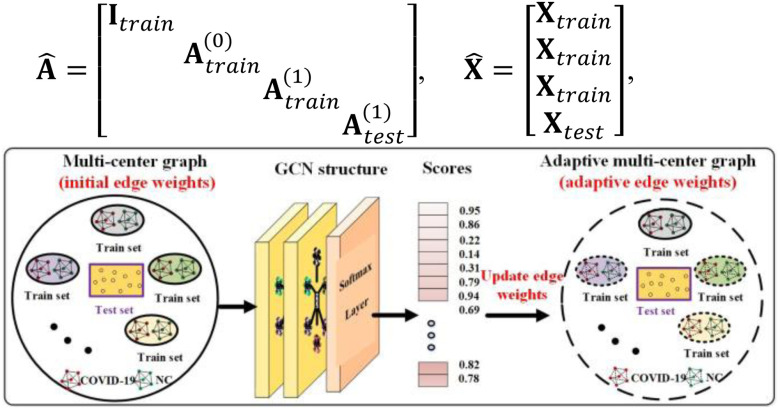
Fig. 2 shows an overview of the proposed diagnosis system. First, we design a multitask 3-D-GCNN framework for extracting features, where the ghost module and the tasks of predicting phenotypic information (i.e., age and sex) are integrated into 3-D-CNN to improve its training. Second, based on the image heterogeneity between different medical centers, we design a multicenter graph, where information such as medical center, disease status, equipment type, and sex is considered. In addition, we propose a novel data augmentation via a multicenter graph, which combines original features, our multicenter graph, and an adaptive multicenter graph. Third, we input the augmented multicenter graph into GCN for final prediction. The summary of important notations in this article is given in Table I.

Fig. 2.

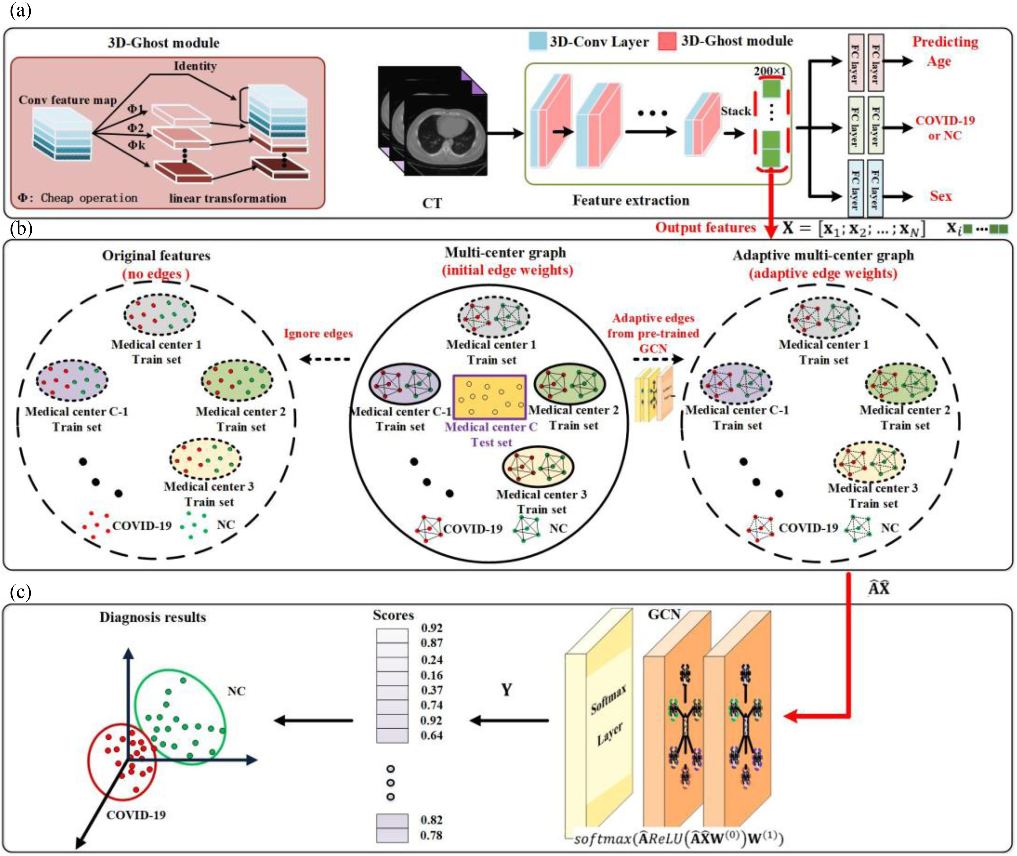
Overview of the proposed framework for COVID-19 diagnosis. (a) Several medical centers’ data is used as training sets to train our multitask 3-D-GCNN, and then the trained model is used to extract features for all subjects. (b) We use the extracted features and phenotypic information to construct multicenter graph, then combine it with the original features and adaptive multicenter graph to form the augmented multi-center graph, where only training samples are augmented. (c) We input the augmented multi-center graph into GCN structure. Finally, every subject in test set is assigned a score for final diagnosis. Note that NC means normal case, and a node on the graph means a subject (represented by its features).

TABLE I. Summary of Important Notations.

Notation	Size	Description
		Total number of medical centers
		Total number of subjects
K		Total number of extracted features for a subject
		Multicenter feature matrix
		Augmented multicenter feature matrix
		Multicenter adjacency matrix
		Augmented multicenter adjacency matrix
		Label matrix

A. Problem Formation

For the task of COVID-19 diagnosis based on multi-center datasets, the main aim of our research is to capture the heterogeneity between datasets and get a robust classifier. Let denote the ground truth label matrix, and are weight coefficient matrices. Then the popular two-layer GCN model [21] is as follows:

The initial input data is a 3-D CT image. The first goal is to extract features from the 3-D CT images to reduce their dimension. By using our multi-task 3-D-GCNN framework for extracting features, every subject is then represented by a feature vector, and all subjects are represented by (total N subjects and everyone has K features), where is the feature vector of subject i.

The second goal is to design the adjacency matrix , which acts as a filter and directly decides the performance of GCN. In this article, we use to present medical centers’ information, and we integrate the information into the construction of our multicenter adjacency matrix to capture the heterogeneity between datasets.

The third goal is to deal with the insufficiency of samples, and we further propose an augmentation mechanism for training samples by designing an augmented multicenter feature matrix and an augmented multi-center adjacency matrix .

B. Multitask 3-D-GCNN for Feature Extraction

In view of the success of the ghost module [24] and the limitation of memory and computation resources, we propose integrating the ghost module into 3-D-CNN [25] to generate more feature maps from simple operations to improve performance. We first use z-score standardization to process the initial CT scans. Since the acquired datasets are nonuniform and the 3-D CT images are of different sizes, we convert all 3-D CT images into the same size of 64 × 64 × 32. Then, these 3-D CT images serve as the input to our multitask 3-D-GCNN. The parameters of convolutional kernels in the 3-D-CNN module are C15@3 × 3 × 3, C25@3 × 3 × 3, C50@3 × 3 × 3, C50@3 × 3 × 3, C100@3 × 3 × 3, C200@3 × 3 × 3, successively. The size of six pooling layers is P2 × 2 × 2. The structure of the 3-D ghost module has a kernel size of 3, and the compression ratio is 2.

For our COVID-19 diagnosis task based on 3-D CT images, insufficiency of samples is a limitation for the final performance. Multitask learning will help to improve network training. In view that sex and age information is usually acquired, we propose a multitask mechanism by adding tasks of predicting age and sex. As shown in Fig. 2, we have two fully connected layers to process the extracted features for every prediction task.

After training the multitask 3-D-GCNN by using the samples from several medical centers, we input all medical centers’ samples into the trained framework. After six convolutional layers and six max-pooling layers, we stack the features and then get a 200 × 1 feature vector. To further reduce the dimension of the feature vector, we use the recursive feature elimination [26] to select the most discriminative features from the 200 × 1 feature vector which leads to a low-dimensional feature vector for every subject.

C. Augmented Multicenter Graph

After extracting features via multitask 3-D-GCNN, we use the features to construct an augmented multicenter graph based on graph theory where every subject is represented by a node. Specifically, we first design a multicenter graph to combine multi-center datasets on a graph. Then we propose to augment the multi-center graph to fit in the few-shot learning task. To improve computational efficiency, we further sparse edges.

1). Multicenter Graph

As the graph in CGN establishes edges between nodes on it and utilizes these edges to realize filtering, designing reasonable edges is the key to capture the heterogeneity between datasets. Hence, we propose to divide all subjects (represented by nodes on graph) into several clusters in the multicenter graph, where every cluster represents all subjects from the same medical center. We establish edge connections between those nodes in the same cluster and ignore the edges between those nodes in different clusters. The details of the filtering principle of graph theory can be seen in the article [22], [23]. Existing studies [22], [23] ignore the disease status of training samples on the graph, which affects convolution performance. Hence, we propose to establish edge connections between those training samples from the same medical center and with the same disease status. For test samples, we establish connections between each pair of them as their status is unknown. Sex and acquired equipment type information is also considered in our multicenter graph.

Let represent the total number of subjects, feature matrix represent their features, and all edge weights compose multi-center adjacency matrix . represents the edge weight between subject and subject , sim denotes the similarity of feature information, represents the distance of sex, represents the distance of equipment type, represents the distance of medical center, and represents the distance of disease status. For subject and subject , and represent their feature vectors, and represent their sex, and represent their equipment types, and represent their medical centers, and and represent their disease status. The corresponding edge weights for the established edges on the multicenter graph are calculated as

The initial similarities are calculated as [22]

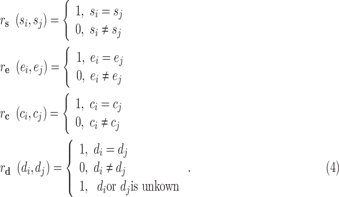
where ρ() is the correlation distance function and σ is the width of the kernel. , , , and are defined as

After constructing the multi-center graph and initializing the edge weights, we get the initial multicenter graph .

2). Augmentation Mechanism

There are a total of 401633 parameters in our multitask 3-D-GCNN framework, which makes the COVID-19 diagnosis as a few-shot learning task and results in many noises on the extracted features. To address it, data augmentation is a popular method. Therefore, we propose an augmented multicenter graph to improve the robustness of a GCN classifier, which augments the training data on the graph. Our augmented multicenter graph includes original features with no edge between nodes, an initial multi-center graph, and an adaptive multicenter graph. The adaptive multicenter graph is shown in Fig. 3. First, we base on (2), (3) and (4) to construct the initial graph. Second, we pre-train the GCN with the initial graph and then get a score for every subject. Third, by using the difference between these scores construct updated similarities, we finally get an adaptive multi-center adjacency matrix, and form an adaptive multicenter graph. The adaptive similarities are computed using

where and denote the scores of subject and subject . is the width of the kernel.

Fig. 3.

Overview of the construction of adaptive multi-center graph.

Finally, all edge weights on the augmented multi-center graph compose an augmented multi-center adjacency matrix and an augmented feature matrix . Then, we get an augmented multicenter graph . and . Let divide into where represents the feature matrix of total subjects in training datasets, and represents the feature matrix of total subjects in the test dataset. Then, , . After augmentation, augmented feature matrix , and augmented multi-center graph ], where is an identity matrix representing the retaining of the original features from training samples. is the initial traditional adjacency matrix calculated based on (2), (3) and (4) for training samples. is our adaptive adjacency matrix calculated based on (2), (4) and (5) for training samples. is our adaptive adjacency matrix for test samples. In our code, and are constructed as

3). Sparse Processing

Sparse representation provides a useful tool for dimensionality reduction and improving computational efficiency [27]. Since dense adjacency matrix in our augmented multi-center graph is of high dimension and this matrix consumes much running time [28], we sparse it by retaining the top edge connections for every node.

The two-layer GCN model [21], [22] is trained using the whole graph as input, and the disease status of test samples (unlabeled on graph) is predicted during training.

III. Experiments and Results

Table II lists seven datasets from different medical centers, including six domestic datasets, and one public dataset. Sex and age information in our six domestic datasets is known whereas the two pieces of information are unknown in the public dataset. As multitask 3-D-GCNN for feature extraction needs sex and age information to improve its training process, we design seven tasks as given in Table III. In tasks 1–6, five of our six domestic datasets are used for training and the other domestic dataset is used for test. In task 7, six domestic datasets are used for training and the other public dataset is used for test. AM-GCN parameters used in experiments are based on the work [22].

TABLE II. Information of Seven Datasets Used in Experiments.

(Wuhan Keting1: 417 COVID-19 + 417 NCs)
(Wuhan Keting2: 178 COVID-19 + 178 NCs)
(Wuhan Seventh Hospital: 104 COVID-19 + 104 NCs)
(Wuhan Shelter: 130 COVID-19 + 130 NCs)
(Wuhan University Zhongnan Hospital: 205 COVID-19 + 205 NCs)
(Harbin Medical University: 79 COVID-19 + 79 NCs)
(Public dataset: 1110 COVID-19 + 1108 NCs) https://mosmed.ai/datasets/covid19_1110
Total: 2223 COVID-19 + 2221 NCs

TABLE III. Information of Our Seven Tasks by Using Several Datasets for Training and One Dataset for Test.

Task	Train set	Test set
Task 1	+ + + +
Task 2	+ + + +
Task 3	+ + + +
Task 4	+ + + +
Task 5	+ + + +
Task 6	+ + + +
Task 7	+ + + + +

A. Performance of Our Multitask 3-D-GCNN

The proposed multitask 3-D-GCNN for COVID-19 diagnosis is evaluated by comparing it with traditional 3-D-CNN. Table IV gives the performance on every single medical center's dataset by five-fold cross-validation, and Table V lists the performance for our seven tasks. As the main task is to diagnose COVID-19, the results of predicting age and sex are not described. As shown in Table IV, compared to traditional 3-D-CNN, 3-D-ResNet, and 3-D-VGG have similar performance, and the proposed multitask 3-D-GCNN in tasks 1–6 has slight performance improvement, with the mean accuracy (ACC) of the six tasks increased by 0.78%, the mean sensitivity (SEN) increased by 1.37%, and the mean specificity (SPE) increased by 0.23%. Table V gives our multitask 3-D-GCNN has significant performance improvement, with the mean ACC of the seven tasks increased by 3.79%, the mean SEN increased by 2.85%, and the mean SPE increased by 4.74%. The significant performance improvement in Table V validates the effectiveness of our method on the tasks of using different datasets for training and test. By using our multitask 3-D-GCNN, the mean ACC in Table IV is 96.73%, whereas the mean ACC in Table V is 90.74%. The obvious difference shows that it is difficult to diagnose COVID-19 by using different medical center datasets for training and test. In contrast, it has good diagnosis performance by using a single medical center dataset for training and test.

TABLE IV. Diagnosis Performance on Single Dataset (%).

Dataset Model		ACC	SEN	SPE	F-score	BAC
	3-D-CNN	99.04	99.51	98.59	99.03	99.05
	3-D-VGG	98.61	100	97.22	98.63	98.61
	3-D-ResNet	97.22	97.14	97.29	97.14	97.22
	Multitask 3-D-GCNN	99.16	99.51	98.82	99.15	99.17
	3-D-CNN	97.22	96.30	98.25	97.30	97.27
	3-D-VGG	98.21	97.59	98.82	98.18	98.20
	3-D-ResNet	98.80	100	97.75	98.75	98.87
	Multitask 3-D-GCNN	97.77	97.96	97.61	97.92	97.78
	3-D-CNN	94.28	90.84	97.13	93.74	93.98
	3-D-VGG	95.23	87.50	100	93.33	93.75
	3-D-ResNet	92.85	89.47	95.65	91.89	92.56
	Multitask 3-D-GCNN	94.76	93.57	95.36	94.18	94.46
	3-D-CNN	95.38	95.43	95.16	95.49	95.30
	3-D-VGG	97.22	94.11	100	96.96	97.05
	3-D-ResNet	97.22	97.14	97.29	97.14	97.22
	Multitask 3-D-GCNN	97.30	96.97	97.56	97.37	97.27
	3-D-CNN	97.28	98.97	95.83	97.17	97.40
	3-D-VGG	96.29	100	93.18	96.10	96.59
	3-D-ResNet	97.53	100	95.55	97.29	97.77
	Multitask 3-D-GCNN	98.27	100	96.75	98.19	98.37
	3-D-CNN	92.50	92.68	92.12	93.54	92.40
	3-D-VGG	90.62	90	91.66	92.30	90.83
	3-D-ResNet	90.62	94.11	86.66	91.42	90.39
	Multitask 3-D-GCNN	93.12	93.95	92.41	94.20	93.18
	3-D-CNN	99.54	99.54	99.55	99.54	99.54
	3-D-VGG	98.87	99.11	98.63	98.89	98.87
	3-D-ResNet	99.32	99.55	99.09	99.32	99.32
	Multitask 3-D-GCNN	/	/	/	/	/

TABLE V. Diagnosis Performance on Our Seven Tasks (%).

Task	Model	ACC	SEN	SPE	F-score	BAC
Task 1	3-D-CNN	92.40	96.20	88.60	92.68	92.40
	3-D-VGG	92.40	100	84.81	92.94	92.40
	3-D-ResNet	87.97	94.93	81.01	88.75	87.75
	Multitask 3-D-GCNN	94.30	100	88.61	94.61	94.30
Task 2	3-D-CNN	88.04	82.44	93.65	87.33	88.04
	3-D-VGG	88.78	85.36	92.19	88.38	88.78
	3-D-ResNet	86.82	76.58	97.07	85.32	96.82
	Multitask 3-D-GCNN	92.19	89.75	94.63	92.00	92.19
Task 3	3-D-CNN	93.46	90.76	96.15	93.28	93.46
	3-D-VGG	93.07	87.69	96.42	92.68	93.07
	3-D-ResNet	93.84	89.23	98.46	93.54	93.84
	Multitask 3-D-GCNN	94.23	90.76	97.69	94.02	94.23
Task 4	3-D-CNN	72.11	92.30	51.92	76.80	72.11
	3-D-VGG	67.30	90.76	43.26	73.64	67.30
	3-D-ResNet	68.26	91.34	45.19	74.21	68.26
	Multitask 3-D-GCNN	78.36	86.53	70.19	80	78.36
Task 5	3-D-CNN	85.11	87.64	82.58	85.47	85.11
	3-D-VGG	84.83	79.77	89.88	84.02	84.83
	3-D-ResNet	83.98	80.89	87.07	83.47	83.98
	Multitask 3-D-GCNN	88.48	82.58	94.38	87.76	88.48
Task 6	3-D-CNN	82.13	65.22	99.04	78.49	82.13
	3-D-VGG	83.57	68.34	98.80	80.62	83.57
	3-D-ResNet	80.93	62.58	99.28	76.65	80.93
	Multitask 3-D-GCNN	91.48	83.69	99.28	90.76	91.48
Task 7	3-D-CNN	95.40	91.34	99.46	95.20	95.39
	3-D-VGG	91	82.00	100	90.10	91
	3-D-ResNet	94.45	88.90	100	94.12	94.44
	Multitask 3-D-GCNN	96.16	92.60	99.73	96.02	96.16

B. Performance of Augmented Multicenter GCN

The performance of the augmented multicenter GCN is evaluated in this subsection. The comparison methods include: multilayer perceptron (MLP), random forests (RFs), gradient boosting decision tree (GBDT), and traditional GCN [22]. M-GCN represents traditional GCN with our multi-center graph, and AM-GCN represents GCN with our augmented multi-center graph. Besides, we use the baseline to represent the proposed multitask 3-D-GCNN. The results of performance comparison are shown in Table VI, and Fig. 4 shows their ROC curves.

TABLE VI. Diagnosis Performance Comparison Based on Extracted Features From Multitask 3-D-GCNN (%).

Task	Model	ACC	SEN	SPE	F-score	BAC
Task 1	Baseline	94.30	100	88.61	94.61	94.30
	MLP	95.56	91.13	100	95.36	95.56
	RF	94.93	90	100	94.73	95
	GBDT	94.30	88.60	100	93.95	94.30
	GCN	96.83	93.67	100	96.73	96.83
	M-GCN	97.46	94.93	100	97.40	97.46
	AM-GCN	98.10	96.20	100	98.06	98.10
Task 2	Baseline	92.19	89.75	94.63	92.00	92.19
	MLP	90.48	97.07	83.90	91.07	90.48
	RF	89.26	94.14	84.39	89.76	89.26
	GBDT	88.78	94.63	82.92	89.40	88.78
	GCN	92.92	95.60	90.24	93.11	92.92
	M-GCN	96.58	97.07	96.09	96.60	96.58
	AM-GCN	98.78	97.56	100	98.76	98.78
Task 3	Baseline	94.23	90.76	97.69	94.02	94.23
	MLP	93.07	99.23	86.92	93.47	93.07
	RF	92.30	99.23	85.38	92.80	92.30
	GBDT	91.15	99.23	83.07	91.81	91.15
	GCN	94.61	99.23	90	94.85	94.61
	M-GCN	98.07	100	96.15	98.11	98.07
	AM-GCN	98.84	100	97.69	98.85	98.84
Task 4	Baseline	78.36	86.53	70.19	80	78.36
	MLP	80.28	73.07	87.50	78.75	80.28
	RF	78.36	69.23	87.50	76.19	78.36
	GBDT	79.32	71.15	87.50	77.48	79.32
	GCN	80.76	75.96	85.57	79.79	80.76
	M-GCN	92.30	95.19	89.42	92.52	92.30
	AM-GCN	94.23	98.07	90.38	94.44	94.23
Task 5	Baseline	88.48	82.58	94.38	87.76	88.48
	MLP	87.41	99.76	75.06	88.79	87.41
	RF	86.69	93.28	80.09	87.51	86.69
	GBDT	85.37	90.88	79.85	86.13	85.37
	GCN	88.60	83.21	94.00	87.95	88.60
	M-GCN	95.20	100	90.40	95.42	95.20
	AM-GCN	96.40	100	92.80	96.52	96.40
	Baseline	91.48	83.69	99.28	90.76	91.48
	MLP	91.01	93.82	88.20	91.25	91.01
	RF	90.73	93.25	88.20	90.95	90.73
Task 6	GBDT	90.73	93.25	88.13	91.00	90.71
	GCN	92.13	91.57	92.69	92.09	92.13
	M-GCN	96.91	98.31	95.50	96.95	96.91
	AM-GCN	98.03	98.31	97.75	98.03	98.03
Task 7	Baseline	96.16	92.60	99.73	96.02	96.16
	MLP	94.53	99.27	89.80	94.78	94.53
	RF	95.08	100	90.16	95.31	95.08
	GBDT	95.03	100	90.07	95.27	95.03
	GCN	95.12	98.46	91.78	95.28	95.12
	M-GCN	96.25	97.74	94.76	96.30	96.25
	AM-GCN	99.77	100	99.54	99.77	99.77

Fig. 4.

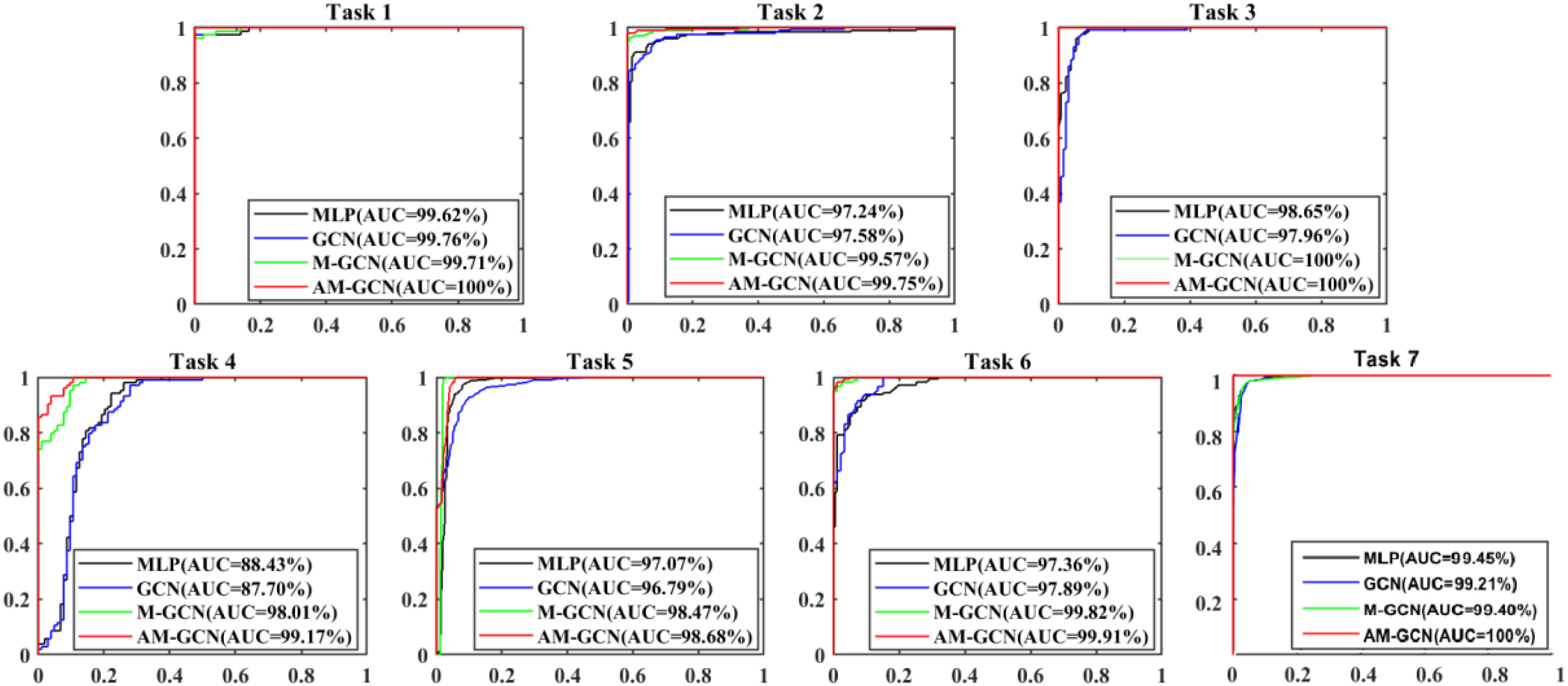
ROC curves of different methods in our seven tasks.

As given in Table VI, the mean ACC of the seven tasks based on Baseline, MLP, RF, and GBDT is 90.74%, 90.33%, 89.62%, and 89.23%, respectively. This shows that using traditional classifiers (e.g., MLP, RF, and GBDT) based on extracted features has no effect on performance improvement compared with using multitask 3-D-GCNN directly for diagnosis. Compared to RF and GBDT, MLP shows better performance.

Compared to MLP, the traditional GCN has slight performance improvement, with the mean ACC of the seven tasks increased by 1.23%, the mean SEN decreased by 1.95%, and the mean SPE increased by 4.69%. By considering the heterogeneity between different datasets, we design our multicenter graph. Compared the performance of M-GCN with that of GCN, the mean ACC of the seven tasks increases by 4.54%, the mean SEN increases by 6.50%, and the mean SPE increases by 2.58%. These results show that our multicenter graph improves performance significantly. For the few-shot learning task, we further propose our augmentation mechanism. Compared the performance of AM-GCN with that of M-GCN, the mean ACC of the seven tasks increases by 1.65%, the mean SEN increases by 0.98%, and the mean SPE increases by 2.32%. These results show that our augmentation mechanism further improves performance slightly. In general, by using our augmented multicenter graph, the performance of GCN receives significant improvement, with the mean ACC of the seven tasks increased by 6.20%, the mean SEN increased by 7.48%, and the mean SPE increased by 4.90%. Finally, it achieves good performance with the mean ACC, SEN, SPE, and AUC of our seven tasks reaching 97.76%, 98.58%, 96.94%, and 99.64%.

C. Filtering Effect of Our Multicenter Graph on the Extracted Features

As there are no related works to evaluate the filter effect of GCN series methods, we propose to describe it by comparing with . represents a multicenter feature matrix that is composed of all subjects’ feature vectors, is our multicenter adjacency matrix, and can also represent the feature matrix after filtering. Fig. 5 presents the filter effect on the extracted top six most discriminative features. In Fig. 5, the blue lines represent the original feature values, which show big fluctuations that make the prediction task difficult. The red lines represent the filtered feature values, which show relatively small fluctuations and provide the foundation for performance improvement.

Fig. 5.

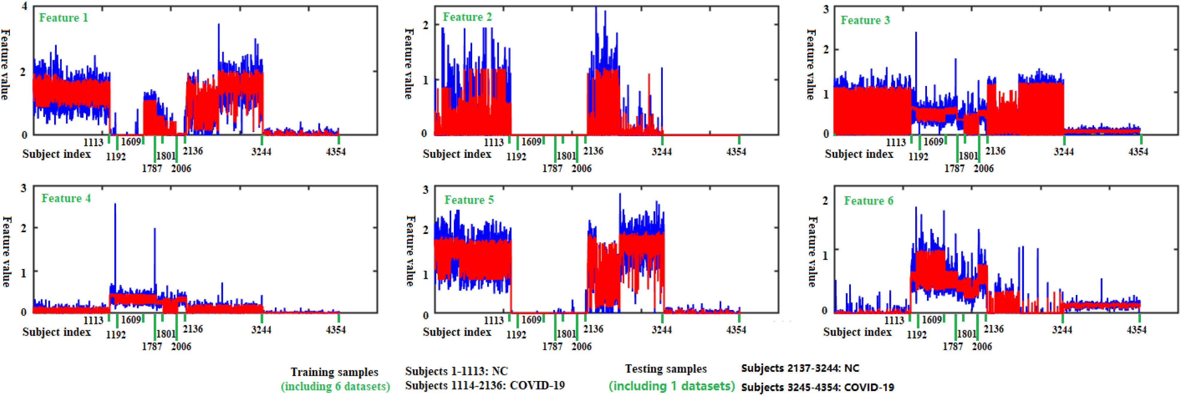
Filtering effect of our multicenter graph on the extracted top 6 most discriminative features by comparing with . Blue lines represent original feature values, and red lines represent filtered feature values.

As shown in Fig. 5 and Table VII, there is much difference in the mean values of the same features between different medical centers’ samples. For example, the mean values of feature 3 for those COVID-19 patients in our seven medical centers are 1.28, 1.04, 1.02, 0.70, 0.28, 0.98, and 0.18, respectively. The mean values of feature 6 for those COVID-19 patients in our seven medical centers are 2.95, 3.24, 2.98, 2.16, 1.69, 2.67 and 0.61, respectively. This difference clearly shows that there is a significant difference in those CT images from different medical centers, which supports the existence of inter-center heterogeneity.

TABLE VII. Mean Feature Values of Subjects in Different Datasets (Computed by Using Original Feature Values).

Feature	NC (All)	COVID in	COVID in	COVID in	COVID in	COVID in	COVID in	COVID in
Feature 1	1.28	0.02	0.00	0.22	0.27	0.03	0.14	0.02
Feature 2	0.03	0.00	0.00	0.00	0.00	0.00	0.00	0.00
Feature 3	0.92	1.28	1.04	1.02	0.70	0.28	0.98	0.18
Feature 4	0.23	2.16	1.65	1.66	1.23	0.34	1.46	0.06
Feature 5	2.71	0.00	0.00	0.00	0.00	0.00	0.21	0.02
Feature 6	0.05	2.95	3.24	2.98	2.16	1.69	2.67	0.61

IV. Discussion

A. Multitask Mechanism

The multitask learning [29] is a popular method in transfer learning, and it is typically done with either hard or soft parameter sharing of hidden layers [30], where hard parameter sharing helps to improve generalization and greatly reduces the risk of overfitting [31]. In view that there are almost 400 thousands of parameters in our 3-D-GCNN framework and only several thousands of samples in our datasets, we propose the multitask mechanism (belonging to hard parameter sharing) by adding tasks of predicting age and sex as assistant tasks. This multitask mechanism is also validated by the work [32], where predicting age and sex are also used as assistant tasks to help train the mild cognitive impairment diagnosis system.

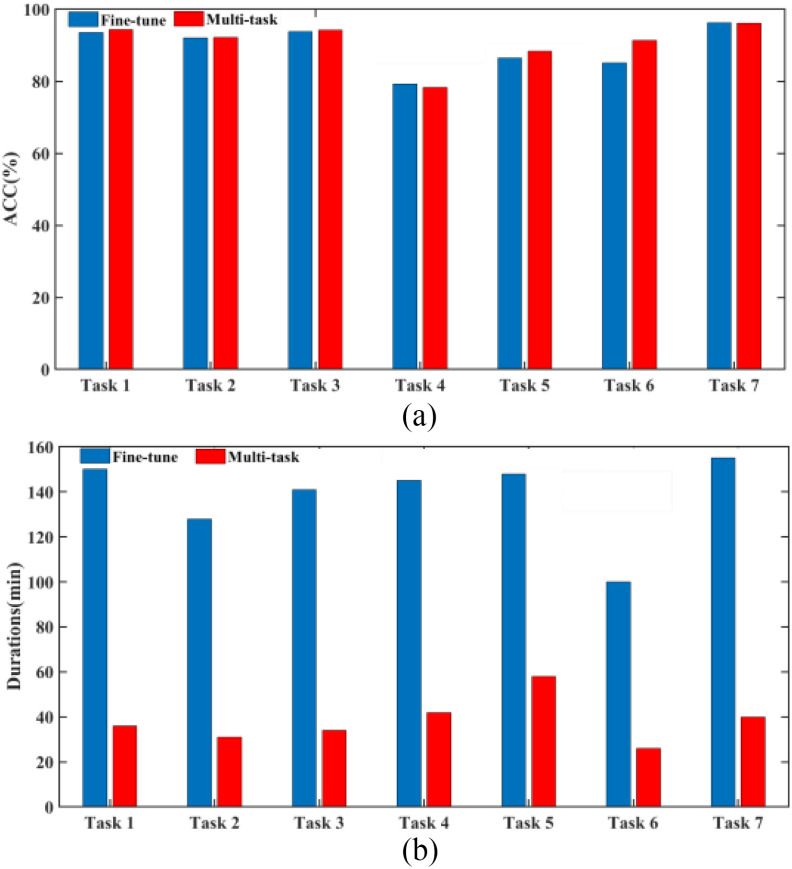
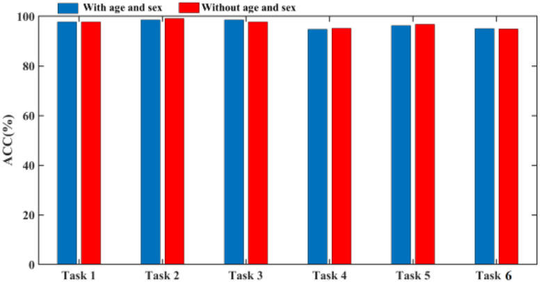
To better show the performance of our multitask learning, we compare it with the widely used fine-tune method which uses tasks of predicting age and sex to pretrain 3-D-GCNN framework, and test the effect of adding related information as additional inputs. As shown in Fig. 6, the mean ACC of the seven tasks is 89.52% for the fine-tune method whereas the mean ACC is 90.74% for our multitask mechanism, and this shows a 1.2% improvement in ACC by using the multi-task mechanism. Compared to a little improvement in ACC, it shows a big improvement in program running time. For details, by using a computer (CPU is Intel(R) Core(TM) i7-8700@3.20GHz, and Keras deep learning library), the mean program running time of the seven tasks is 138 minutes for the fine-tune method, whereas the mean program running time is 38 min for our multitask mechanism. This shows the fine-tune method consumes much more time. To show the effect of treating age and sex as additional inputs in the COVID-19 diagnosis system, we use 3-D-GCNN to extract features from 3-D CT images where the fine-tune method is applied to pretrain the system, and then compare the diagnosis results of GCN classifier with and without adding age and sex as input features. As shown in Fig. 7, there is no improvement in ACC by adding age and sex as input features where the mean ACC is 96.9% and 96.8% with and without adding them as input features. This result is consistent with the work [32] that simply adding sex and age as additional inputs will probably not improve performance.

Fig. 6.

Diagnosis performance and program running time comparison between fine-tune method and multitask mechanism based on 3-D-GCNN. (a) Diagnosis performance comparison. (b) Program running time comparison.

Fig. 7.

Diagnosis performance comparison with and without age and sex as additional inputs in a GCN classifier.

B. Validation Strategy

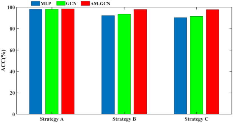
There are three popular validation strategies for multicenter learning as shown in Fig. 8 [16], [17]. Compared to strategy A and strategy B, strategy C has a higher request on classifiers and we pick it as our validation strategy in the above experiments. To better show the effectiveness of our method, we also show the diagnosis results for strategies A and B. Specifically, in strategy A, we separate every dataset into 80% and 20% for training and test. In strategy B, 80% of the samples in one dataset are used for test and the others are used for training. In strategy C, one dataset is selected for test, while the others are used for training.

Fig. 8.

Popular validation strategies for multicenter learning.

The diagnosis results based on the above three validation strategies are shown in Fig. 9. By using the MLP classifier, the mean ACC for strategies A, B, and C is 98.2%, 92.2%, and 90.3%, respectively. This result shows that strategy C has a higher request on classifiers which makes the lowest ACC, whereas strategy A makes the best ACC. Compared to MLP, by using traditional GCN, the mean ACC in strategy A decreases by 0.01%, whereas the mean ACC in strategy B and C increases by 1.31% and 1.24%. By using our AM-GCN, the mean ACC in strategies A, B, and C increases by 0.23%, 5.61%, and 7.4%. This result shows that our AM-GCN can improve performance significantly for strategy B and C, whereas it has little effect on performance improvement for strategy A.

Fig. 9.

Diagnosis results based on three validation strategies.

C. Effect of Sparse Processing

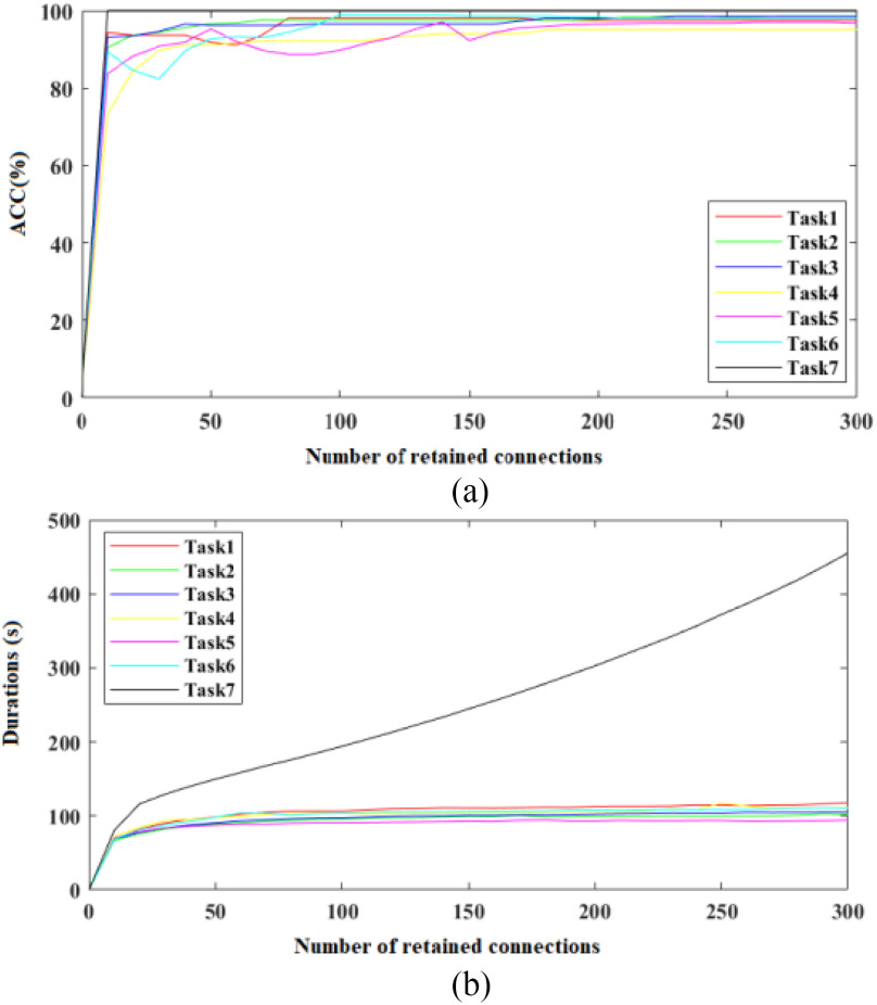
As there are thousands of subjects on the augmented multicenter graph in diagnosis tasks, we use a sparse adjacency matrix to improve the computational efficiency of AM-GCN. Fig. 10 shows the effect of the sparse processing on accuracy and program running time. The used CPU is Intel(R) Core(TM) i7-8700@3.20 GHz. As the adjacency matrix in traditional GCN is a high dimensional dense adjacency matrix, where all edge connections are retained. By using our multicenter graph, some connections have been discarded and this makes our adjacency matrix sparse. By using sparse processing, we further reduce the number of edge connections. As shown in Fig. 10, the number of retained edge connections significantly affects program running time. Running programs will consume more time if we retain more edge connections. To balance good performance on diagnosis accuracy and time cost, we finally retain 200 edge connections for every node on the graph in experiments.

Fig. 10.

Effect of number of retained edge connections on accuracy and program running time. (a) Effect on accuracy. (b) Effect on program running time.

D. Effect of Phenotypic Information

In the traditional GCN method for predicting Alzheimer's disease [22], phenotypic information (e.g., sex and equipment type) shows an effect on accuracy with a 3% improvement in accuracy by including them. In this subsection, we test their effect on our AM-GCN. sim denotes the similarity of image information, and the details of integrating phenotypic information into AM-GCN are shown in (2). Table VIII gives there are few variations on ACC between different combination strategies for all seven tasks. Specifically, for tasks 3, 4, 5, and 7, phenotypic information shows no effect on final diagnosis accuracy. For task 1 and task 6, by including equipment information, the ACC increases by 0.63% and 0.31%, whereas it shows no effect on performance improvement by including sex information. For task 3, including sex and equipment information deteriorates performance. The above results show that phenotypic information (e.g., equipment type and sex) has little effect on final diagnosis performance in our tasks.

TABLE VIII. Effect of Phenotypic Information on Diagnosis Accuracy (%).

Phenotypic info.	Task 1 Task 2 Task 3 Task 4 Task 5 Task 6							Task 7
Sim		97.47	98.78	98.84	94.23	96.40	97.72	98.51
Sim+Equip		98.10	98.78	98.84	94.23	96.40	98.03	99.77
Sim+Sex		97.47	98.54	98.84	94.23	96.40	97.72	99.77
Sim+Sex+Equip		98.10	98.54	98.46	94.23	96.40	97.84	99.77

E. Comparison With the Related Works

Table IX gives the diagnosis performance of our method and related methods. These related works use CNN series methods for COVID-19 diagnosis, treat multicenter data as one dataset, and use five- or ten-fold cross-validation to validate their methods. By adjusting network structure, using transfer learning to improve the training process, and using GAN to augment data, good diagnosis performance has been achieved. But these processes ignore the heterogeneity between different datasets, which limits the final performance to some extent. And our work aims to study the heterogeneity between different datasets to improve final performance. Different from the used five- or ten-fold cross-validation in related methods, we use different datasets for training and test. In our experiment, there are six in-house datasets and one public dataset from different medical centers. A total of 2223 COVID-19 patients and 2221 NCs are collected, which is more than the acquired samples in related works (e.g., 110 [4], 413 [7], 1296 [8], and 2148 [13] COVID-19 patients) and makes our experimental results convincing. Although our validation strategy is much more difficult than related works, it is observed that our method achieves the mean ACC of 97.76% which is better than the methods in those related works that bases on CT images (e.g., 93.1% [7], 91.9% [2], and 89.79% [13]). Compared to related works that mainly analyze the influence of adaptive feature selection method [2], few labeled data [13], and their method [5], [8], our work analyses the effect of phenotypic information, the difference of extracted features between different datasets, and the filtering effect of our multi-center graph. The major difference of extracted features between different datasets validates that there is much heterogeneity in those images from different medical centers. By addressing it, our AM-GCN achieves good performance.

TABLE IX. Algorithm Comparison With the Related Works (%).

Ref.	Modality	Method	Subject	ACC SEN SPE
[3]	X-ray	DarkNet model	2 Center: 127 COVID-19, 500 NC.	98.08	95.13	95.3
[6]	X-ray	ResNet50	1 Center: 25 COVID-19, 25 NC.	95.38	97.29	93.47
[10]	X-ray	Shuffled residual CNN	7 Center: 392 COVID-19, 392 NC.	99.80	99.94	98.01
[11]	X-ray	SqueezeNet	2 Center: 84 COVID-19, 100 NC.		98	92.9
[14]	X-ray	InstaCovNet-19	2 Center: 361 COVID-19, 365 NC.	99.52
[2]	CT	Adaptive Feature Selection, Deep Forest	5 Centers: 1495 COVID-19, 1027 CAP.	91.79	93.05	89.95
[4]	CT	3-D-CNN, Location attention oriented model	3 Center: 110 COVID-19, 175 NC.	/	98.2	92.2
[5]	CT	CNN, MLP, SVM	18 Centers: 419 COVID-19, 486 NC.	/	84.3	82.8
[7]	CT	ResNet32, Deep transfer learning	2 Center: 413 COVID-19, 439 NC.	93.01	91.45	94.77
[8]	CT	ResNet50	6 Centers: 1296 COVID-19, 1735 CAP, 1325NC.	/	90	96
				/	87	92
				/	94	96
[9]	CT	3-D U-Net++	5 Centers: 723 COVID-19, 1027 CAP.	/	97.4	92.2
[12]	CT	DeCoVNet	3 Centers: 313 COVID-19, 229 Others.	/	90.7	91.1
[13]	CT	Uncertainty Vertex-weighted Hypergraph Learning	5 Centers: 2148 COVID-19, 1182 CAP.	89.79	93.26	84
[15]	CT	Modified Inception transfer-learning model	3 Center: 79 COVID-19, 180 CAP.	89.5	87	88
Ours	CT	Multitask 3-D-GCNN, Augmented multi-center GCN	7 Centers: 2223 COVID-19, 2221 NC.	97.76	98.58	96.94

SVM: Support vector machine.

Additionally, the work [33] focuses on studying the regions that contains the most informative COVID-19 features and introduces a hybrid approach based on the thresholding technique to solve the image segmentation problem. Inspired by the work, we will study to improve our diagnosis performance by integrating the image segmentation task in our future work.

V. Conclusion

By analyzing the extracted features of 3-D CT images from seven different medical centers, it was found that there was much difference in mean values and fluctuations of the same features between different medical centers’ samples. This result validated that there was obvious heterogeneity between those images acquired from different medical centers, which consists of the fact that different medical centers probably utilize different acquisition devices, imaging parameters, and standards. Our multicenter graph could combine all samples from seven medical centers on a graph and establish their interactions. By comparing the filtered features using the multicenter graph, it showed that fluctuations of the same features in different medical centers’ samples could be well suppressed, and this validated the effectiveness of the graph theory. The final performance improvement validated that combining all samples from different medical centers on a graph can enhance the robustness and diagnosis performance of the classifier. By using our augmentation mechanism, the performance is further improved. This showed that the insufficiency of samples was an important limiting factor and data augmentation improves performance. The performance improvement by adding the tasks of predicting age and sex in 3-D-GCNN structure, showed that multitask mechanism was beneficial to network training whereas simply adding sex and age as additional inputs will probably not improve performance. In the three popular validation strategies for multicenter learning, our method improves performance significantly for strategies B and C. By analyzing the effect of sparse processing and phenotypic information, we found that our AM-GCN has good robustness, and graph theory consumes much program running time which can be addressed by sparse processing. The good performance of our AM-GCN mainly lies in its good filtering effect, and it relatively adapts to few-shot learning tasks. The proposed AM-GCN method can be applied to other related classification tasks.

Biographies

Xuegang Song received the Ph.D. degree in instrument science and technology from the Nanjing University of Aeronautics and Astronautics, Nanjing, China, in 2018.

He is currently with the School of Biomedical Engineering, Shenzhen University, China. His research interests include medical image analysis, deep learning, mechanical vibration, and signal processing.

Haimei Li received the B.Sc. degree in clinical medicine from Changzhi Medical College, Changzhi, China, in 2003.

She is currently with the Fuxing Hospital, Capital Medical University, Beijing, China. She has been engaged in the clinical, teaching and scientific research of medical imaging for 30 years, and has a solid basic theory and rich practical experience in the field of medical imaging.

Ms. Li is a Member of the Medical Imaging Engineering and Technology Branch of the Chinese Biomedical Engineering Society and the brain Cognition and Health Branch of the Chinese Geriatrics and Geriatrics Association.

Wenwen Gao received the B.Sc. degree in medical imaging from Qingdao University, Qingdao, China, in 2017. She is currently working toward the M.D. degree with China Japan Friendship Hospital, Beijing, China.

Her current research interests include resting state functional magnetic resonance imaging and radiomics.

Yue Chen received the B.Sc. degree in medical imaging from Dalian Medical University, Dalian, China, in 2019. She is currently working toward the M.D. degree with China-Japan Friendship Hospital, Beijing, China.

Her current research interests include radiomics and application of arterial spin labeling magnetic resonance technique.

Tianfu Wang received the Ph.D. degree in biomedical engineering from Sichuan University, Chengdu, China, in 1997.

He is currently a Professor with Shenzhen University, Shenzhen, China. His current research interests include ultrasound image analysis, medical image processing, pattern recognition, and medical imaging.

Guolin Ma received the M.D. degree from Peking Union Medical College, Beijing, China, in 2013.

He is currently a Chief Radiologist with the Department of Radiology, China-Japan Friendship Hospital, Beijing, China, and a Professor with the Department of Medicine, Peking University, Beijing, China. He has authored or coauthored more than 70 articles. His current research interests include basic and clinical application of functional magnetic resonance imaging, artificial intelligence and radiomics, and specialize in imaging diagnosis of neurological and mental disorders.

Dr. Wang is the Vice Chairman of the Medical Imaging Engineering and Technology Branch, Chinese Society of Biomedical Engineering, and the CT Engineering and Technology Special Committee of the China Association of Medical Equipment.

Baiying Lei (Senior Member, IEEE) received the M.Eng. degree in electronics science and technology from Zhejiang University, Hangzhou, China, in 2007, and the Ph.D. degree in information engineering from Nanyang Technological University, Singapore, in 2012.

She is currently with the Health Science Center, School of Biomedical Engineering, Shenzhen University, Shenzhen, China. She has coauthored more than 200 scientific articles published in various journals, e.g., Medical Image Analysis, IEEE Transactions on Medical Imaging, IEEE Transactions on Cybernetics, IEEE Transactions on Neural Networks and Learning Systems, IEEE Transactions on Biomedical Engineering, IEEE Transactions on Computational Imaging, IEEE Journal of Biomedical and Health Informatics, Pattern Recognition. Her current research interests include medical image analysis, machine learning, and pattern recognition.

Dr. Lei is an Editorial Board Member of Medical Image Analysis, Frontiers in Neuroinformatics, and Frontiers in Aging Neuroscience, and an Associate Editor for the IEEE Transactions on Medical Imaging.

Funding Statement

This work was supported in part by the National Natural Science Foundation of China under Grant 61871274, Grant U1909209, and Grant 61801305, in part by Guangdong Pearl River Talents Plan under Grant 2016ZT06S220, in part by Shenzhen Peacock Plan under Grant KQTD2016053112051497 and Grant KQTD2015033016104926, and in part by Shenzhen Key Basic Research Project under Grant JCYJ20180507184647636, Grant JCYJ20170818094109846, and Grant GJHZ20190822095414576.

References

- [1].Zu Z. et al. , “Coronavirus disease 2019 (COVID-19): A perspective from China,” 2020. [Online]. Available: https://doi.org/10.1148/radiol.2020200490 [DOI] [PMC free article] [PubMed]
- [2].Sun L. et al. , “Adaptive feature selection guided deep forest for COVID-19 classification with chest CT,” 2020. [Online]. Available: https://arxiv.org/abs/2005.03264 [DOI] [PMC free article] [PubMed]
- [3].Ozturk T., Talo M., Yildirim E. A., Baloglu U. B., Yildirim O., and Acharya U. R., “Automated detection of COVID-19 cases using deep neural networks with X-ray images,” Comput. Biol. Med., vol. 121, Jun. 2020, Art. no. 103792. [DOI] [PMC free article] [PubMed] [Google Scholar]
- [4].Butt C., Gill J., Chun D., and Babu B. A., “Deep learning system to screen coronavirus disease 2019 pneumonia,” 2020. [Online]. Available: https://doi.org/10.1007/s10489-020-01714-3 [DOI] [PMC free article] [PubMed]
- [5].Mei X. et al. , “Artificial intelligence-enabled rapid diagnosis of patients with COVID-19,” Nat. Med., vol. 26, pp. 1224–1228, May 2020. [DOI] [PMC free article] [PubMed] [Google Scholar]
- [6].Sethy P. K. and Behera S. K., “Detection of coronavirus disease (COVID-19) based on deep features,” 2020. [Online]. Available: https://doi.org/10.20944/preprints202003.0300.v1
- [7].Pathak Y., Shukla P. K., Tiwari A., Stalin S., Singh S., and Shukla P. K., “Deep transfer learning based classification model for COVID-19 disease,” Intermediate-Range Ballistic Missile, 2020. [Online]. Available: https://doi.org/10.1016/j.irbm.2020.05.003 [DOI] [PMC free article] [PubMed]
- [8].Li L. et al. , “Artificial intelligence distinguishes COVID-19 from community acquired pneumonia on chest cT,” Radiology, vol. 296, no. 2, pp. E65–E71, Aug. 2020. [DOI] [PMC free article] [PubMed] [Google Scholar]
- [9].Jin S. et al. , “AI-assisted CT imaging analysis for COVID-19 screening: Building and deploying a medical AI system in four weeks,” 2020. [Online]. Available: https://doi.org/10.1101/2020.03.19.20039354 [DOI] [PMC free article] [PubMed]
- [10].Karthik R., Menaka R., and Hariharan M., “Learning distinctive filters for COVID-19 detection from chest X-ray using shuffled residual CNN,” Appl. Soft Comput., vol. 99, Sep. 2020, Art. no. 106744. [DOI] [PMC free article] [PubMed] [Google Scholar]
- [11].Minaee S., Kafieh R., Sonka M., Yazdani S., and Soufi G. J., “Deep-COVID: Predicting COVID-19 from chest X-ray images using deep transfer learning,” 2020. [Online]. Available: https://arxiv.org/abs/2004.09363 [DOI] [PMC free article] [PubMed]
- [12].Zheng C. et al. , “Deep learning-based detection for COVID-19 from chest CT using weak label,” 2020. [Online]. Available: https://doi.org/10.1101/2020.03.12.20027185
- [13].Di D. et al. , “Hypergraph learning for identification of COVID-19 with CT imaging,” 2020. [Online]. Available: https://arxiv.org/abs/2005.04043 [DOI] [PMC free article] [PubMed]
- [14].Anjum A. G., Gupta S., and Katarya R., “InstaCovNet-19: A deep learning classification model for the detection of COVID-19 patients using chest X-ray,” Appl. Soft Comput., vol. 99, Oct. 2020, Art. no. 106859. [DOI] [PMC free article] [PubMed] [Google Scholar]
- [15].Wang S. et al. , “A deep learning algorithm using CT images to screen for corona virus disease (COVID-19),” 2020. [Online]. Available: https://doi.org/10.1101/2020.02.14.20023028 [DOI] [PMC free article] [PubMed]
- [16].Wang Z., Liu Q., and Dou Q., “Contrastive cross-site learning with redesigned net for COVID-19 CT classification,” IEEE J. Biomed. Health, vol. 24, no. 10, pp. 2806–2813, Oct. 2020. [DOI] [PMC free article] [PubMed] [Google Scholar]
- [17].Wang M., Zhang D., Huang J., Yap P., Shen D., and Liu M., “Identifying autism spectrum disorder with multi-site fMRI via low-rank domain adaptation,” IEEE Trans. Med. Imag., vol. 39, no. 3, pp. 644–655, Mar. 2020. [DOI] [PMC free article] [PubMed] [Google Scholar]
- [18].Huang F. et al. , “Self-weighted adaptive structure learning for ASD diagnosis via multi-template multi-center representation,” Med. Image Anal. , vol. 63, Jul. 2020, Art. no. 101662. [DOI] [PubMed] [Google Scholar]
- [19].Wang J. et al. , “Multi-task diagnosis for autism spectrum disorders using multi-modality features: A multi-center study,” Hum. Brain Mapping , vol. 38, no. 6, pp. 3081–3097, Jun. 2017. [DOI] [PMC free article] [PubMed] [Google Scholar]
- [20].Wachinger C. and Reuter M., “Domain adaptation for Alzheimer's disease diagnostics,” NeuroImage, vol. 139, pp. 470–479, Oct. 2016. [DOI] [PMC free article] [PubMed] [Google Scholar]
- [21].Kipf T. N. and Welling M., “Semi-supervised classification with graph convolutional networks,” 2017. [Online]. Available: https://arxiv.org/abs/1609.02907
- [22].Parisot S. et al. , “Disease prediction using graph convolutional networks: Application to autism spectrum disorder and Alzheimer's disease,” Med. Image Anal. , vol. 48, pp. 117–130, Aug. 2018. [DOI] [PubMed] [Google Scholar]
- [23].Ktena S. I. et al. , “Metric learning with spectral graph convolutions on brain connectivity networks,” NeuroImage, vol. 169, pp. 431–442, Apr. 2018. [DOI] [PubMed] [Google Scholar]
- [24].Han K., Wang Y., Tian Q., Guo J., Xu C., and Xu C., “GhostNet: More features from cheap operations,” in Proc. IEEE Conf. Comput. Vis. Pattern Recognit., 2020, pp. 1580–1589. [Google Scholar]
- [25].Ji S., Xu W., Yang M., and Yu K., “3D convolutional neural networks for human action recognition,” IEEE Trans. Pattern Anal., vol. 35, no. 1, pp. 221–231, Jan. 2013. [DOI] [PubMed] [Google Scholar]
- [26].Guyon I., Weston J., Barnhill S., and Vapnik V., “Gene selection for cancer classification using support vector machines,” Mach. Learn., vol. 46, pp. 389–422, Jan. 2002. [Google Scholar]
- [27].Wang J., Lu C., Wang M., Li P., Yan S., and Hu X., “Robust face recognition via adaptive sparse representation,” IEEE Trans. Cybern., vol. 44, no. 12, pp. 2368–2378, Dec. 2014. [DOI] [PubMed] [Google Scholar]
- [28].Chen P., Jiao L., Liu F., Zhao Z., and Zhao J., “Adaptive sparse graph learning based dimensionality reduction for classification,” Appl. Soft Comput., vol. 82, Sep. 2019, Art. no. 105459. [Google Scholar]
- [29].Pan S. and Yang Q., “A survey on transfer learning,” IEEE Trans. Knowl. Data Eng., vol. 22, no. 10, pp. 1345–1359, Jan. 2010. [Google Scholar]
- [30].Ruder S., “An overview of multi-task learning in deep neural networks,” 2017. [Online]. Available: https//arxiv.org/abs/1706.05098
- [31].Caruana R., “Multitask learning,” Mach. Learn., vol. 28, pp. 41–75, Jul. 1997. [Google Scholar]
- [32].Xing X. et al. , “Dynamic spectral graph convolution networks with assistant task training for early MCI diagnosis,” in Proc. Int. Conf. Med. Image Comput. Comput. Assisted Intervention, 2019, pp. 639–646. [Google Scholar]
- [33].Abdel-Basset M., Chang V., and Mohamed R., “HSMA_WOA: A hybrid novel slime mould algorithm with whale optimization algorithm for tackling the image segmentation problem of chest X-ray images,” Appl. Soft Comput., vol. 95, Oct. 2020, Art. no. 106642. [DOI] [PMC free article] [PubMed] [Google Scholar]