An Effective Deep Neural Network for Lung Lesions Segmentation From COVID-19 CT Images

Abstract

Automatic segmentation of lung lesions from COVID-19 computed tomography (CT) images can help to establish a quantitative model for diagnosis and treatment. For this reason, this article provides a new segmentation method to meet the needs of CT images processing under COVID-19 epidemic. The main steps are as follows: First, the proposed region of interest extraction implements patch mechanism strategy to satisfy the applicability of 3-D network and remove irrelevant background. Second, 3-D network is established to extract spatial features, where 3-D attention model promotes network to enhance target area. Then, to improve the convergence of network, a combination loss function is introduced to lead gradient optimization and training direction. Finally, data augmentation and conditional random field are applied to realize data resampling and binary segmentation. This method was assessed with some comparative experiment. By comparison, the proposed method reached the highest performance. Therefore, it has potential clinical applications.

I. Introduction

Since December 2019, a new coronavirus pneumonia (COVID-19) has constituted a global epidemic threat. It is highly contagious and spreads quickly, causing huge damage to the world health and economy in the short term. As of January 11, 2021, COVID-19 has spread to more than 191 countries and regions around the world, with a total of 90 216 381 confirmed cases, 1 933 487 cases involving deaths, and a mortality rate of about 2.14% [1]. Commonly, viral nucleic acid testing, gene sequencing, and viral antibody serological testing are the gold standard methods for the diagnosis of COVID-19 [2]. However, due to technical limitations, it is impossible to quickly and accurately screen suspected cases. Computed tomography (CT) imaging diagnosis can detect some suspected features, such as single or multiple ground glass-like lesions, solid lesions, and thickened leaflet intervals [3]–[5]. In addition, chest CT examination has the advantages of short time, 3-D structure and high sensitivity, it is currently one of the routine auxiliary examination methods for the screening, diagnosis, and evaluation of COVID-19 [6], [7].

At present, CT imaging diagnosis for COVID-19 depends on the clinical experiences of radiologists [8], [9]. The professional level and the personal judgment of different doctors dominate the inconsistent diagnosis [10]. In addition, radiologists and specialists need to browse more than 300 CT slices of each patient to diagnose and analyze COVID-19 lesions. Because of the pandemic and the shortage of medical resources, the efficiency and accuracy of disease diagnosis present serious challenges [11]–[13]. By CT images segmentation, intuitive 3-D structures and accurate digital models can be obtained [14]. It can quickly locate suspicious COVID-19 lesions and calculate quantitative data, such as volume, shape, and density of the lesions. Thus, it is possible to reduce the burden on doctors and improve work efficiency. It also reduces the time that high-risk patients stay in the hospital to wait for the CT examination results, thereby avoiding cross infection [15]. But the lung lesions of COVID-19 are usually complex with no obvious regularity [16], [17]. Fig. 1 shows the coronal slices of two sets of CT images. In order to show clearly, lesions part was enlarged locally, where one of them reveals that lesions adhere to tissues and vessels [see Fig. 1(a) and (c)]. Another is lesions which grow into sprawling [see Fig. 1(d) and (f)]. Thus, how to extract lung lesions from COVID-19 CT images effectively and accurately is still a difficult challenge.

Fig. 1.

CT images of a COVID-19 infected lung. (b) and (e) are the original CT images; (a) and (d) represent the local enlargement of the right lungs; (c) and (f) represent the local enlargement of the left lungs.

Many researchers have explored methods to segment lung lesions from COVID-19 CT images. For examples, Fan et al. [18] proposed a lung infection segmentation deep network (Inf-Net) to automatically identify infected areas in CT images. In their work, a semisupervised framework based on random propagation was applied to make up for the lack of data. But it was necessary to manually screen the slices with infected areas. Qiu et al. [19] presented a lightweight model MiniSeg for efficient COVID-19 segmentation to achieve coping with insufficient data and fast training. They simplified the model structure, which had the advantages of light weight and high efficiency, but also brought a certain loss of accuracy. Yan et al. [20] established a new network to analyze the COVID-19 infection. They could improve global energy to enhance the border of infection. Then, a feature mutation module was introduced to adaptively adjust the global attributes of the features used to segment the COVID-19 infection. They introduced the pyramid space fusion function to deal with features of different scales, but it also increased the difficulty of training. Saeedizadeh et al. [21] proposed a segmentation framework to segment the chest area infected by COVID-19 in CT images. A proper regularization term was added to improve the connectivity of the target area. Since they mainly focused on the connected component, this also caused the locally spreading lesion structure to be easily ignored. Abdel-Basset et al. [22] presented a semisupervised model based on few-shot learning for COVID-19 segmentation. Their work solved the problem of insufficient data and realized efficient small sample learning. But the spatial information of the 3-D structure was not considered.

In summary, although there have been some methods for processing COVID-19 CT images, there are still some problems that need further improvement as follows:

• 1)Due to the variable and complex tissue structures of the infected lung area, accurate segmentation is still a challenge;
• 2)Compared with entire lung CT images, the infected area occupies only a small part. Thus, there are mismatches between positive and negative samples.
• 3)The infected area is usually spreading over multiple layers, which means it has 3-D characteristic information.

Therefore, 2-D slice processing methods are not appropriate for the COVID-19 CT images. Also, 3-D structures methods will face huge computational pressure.

To solve these problems, this article proposes a novel method for lesions segmentation from COVID-19 CT images. It mainly includes the following contributions: First, the proposed Region of Interest (ROI) extraction implements patch mechanism strategy to satisfy the applicability of 3-D network and remove redundant background information. Second, 3-D attention model is introduced to extract spatial features and promote network to enhance target area. Finally, to effectively converge this network, a combination loss function is introduced to lead gradient optimization and training direction. This article provides a new segmentation method to meet the needs of CT images processing under COVID-19 epidemic.

II. Methods

This work proposes a novel method to achieve segmentation of COVID-19 infection area. The main steps are as follows: First, infected area is located and cropped by proposed ROI extraction. Then, a new module is added into deep learning model to extract features. Also, data augmentation and combinational loss are applied to improve the performance of model. Finally, conditional random field (CRF) is used to classify the obtained continuous probability distribution and then results are verified and evaluated.

A. ROI Extraction

In COVID-19 infected lungs, the area of lesions is usually less than 5% of the total volume, which is a problem of high data imbalance. To prevent the model from being covered by the background pixel features, focusing on the image features around the target is important. Thus, a localization strategy is proposed to obtain voxel patches with a high proportion of lesion area. Fig. 2 shows the entire process of ROI extraction. The principle of data screening is to display the lesion boundary contour characteristics as much as possible. After measurement, voxel patches of 64×64×64 size can be better satisfied. Because COVID-19 CT images are unified into 512×512 slice size with an indeterminate layer height structure, each slice is divided into eight parts for X-axis and Y-axis. Also, layer height is expressed as , so the number of cuts and the remainder in Z-axis is and . In consideration that the upper and lower layers are mainly background, the remainder is approximately allocated to the upper and lower layers for edge trimming.

Fig. 2.

ROI extraction. The figure shows the process of ROI extraction, which represents voxel patches grayscale histogram, calculation of probability value, probability distribution and center point conversion.

Then, to determine whether the voxel contains lesions, a grayscale histogram of voxel is established. When three cluster centers appear in the gray histogram, lesions are judged to exist, as shown in Fig. 2. Where, 1, 2, and 3 represent lungs, lesions, and tissues, respectively. To ensure sufficient lesion areas and cover the boundary contour, calculation method is given as follows:

where represents the probability of the selected node, represents the non-lesion area, and indicates distance from nonnodes to nodes. The probability value of a nonlesion area is defined as 0, which makes voxels that are close to the lesion contour obtain the maximum probability as a boundary layer. Finally, 60% of are selected as the new boundary points, and one of them is taken as the cutting center.

B. Data Augmentation

To reduce overfitting and realize data resampling, a 3-D voxel enhancement method is adopted to augment data. Fig. 3 shows some examples of data augmentation. In the augmentation strategy, a total of seven methods are adopted, including: random rotation, brightness shift, random spatial shift, random spatial shear, random spatial zoom, elastic transformation, and random channel shift. Random rotation realizes a rotation of the image within the angle range. A brightness shift changes the brightness of the voxels. Random spatial shear completes random cropping. Random spatial zoom can scale a picture randomly. Elastic transformation realizes the random standard deviation of each dimension of pixels. Finally, random channel shift shifts the channel value by a random selected from the specified range. Thus, including the original voxels, an enhancement method is randomly selected in each epoch, and then network training begins.

Fig. 3.

Some examples of data augmentation.

C. 3-D Attention Module

3-D U-Net [23] is a classic network model widely applied in medical image processing. Normally, skip-connection of it is directly transmitted from shallow to deep level. Since features of low latitude contain many background information, the target area cannot be focused. Inspired by [24], to improve the saliency of object, this work proposes a 3-D attention structure to increase the attention to the object. Fig. 4 shows the proposed 3-D attention module. The input feature maps are defined as . The main purpose is to increase the target weight in each . It has been verified that average pooling and maximum pooling are reliable weight calculation methods. Thus, and are defined as output of average pooling layer and maximum pooling layer and calculated, respectively. Then, after average pooling and maximum pooling processing, the final weights are obtained through the 3-D convolutional layer and the sigmoid activation layer. Finally, the weights are multiplied by the input to obtain a weighted feature map in a 3-D space. The main calculation method is expressed as follows:

where denotes the feature map of average pooling, means the feature map of max pooling, is convolution operation with 3 kernel size, and expresses the elementwise multiplication.

Fig. 4.

Illustration of 3-D attention module.

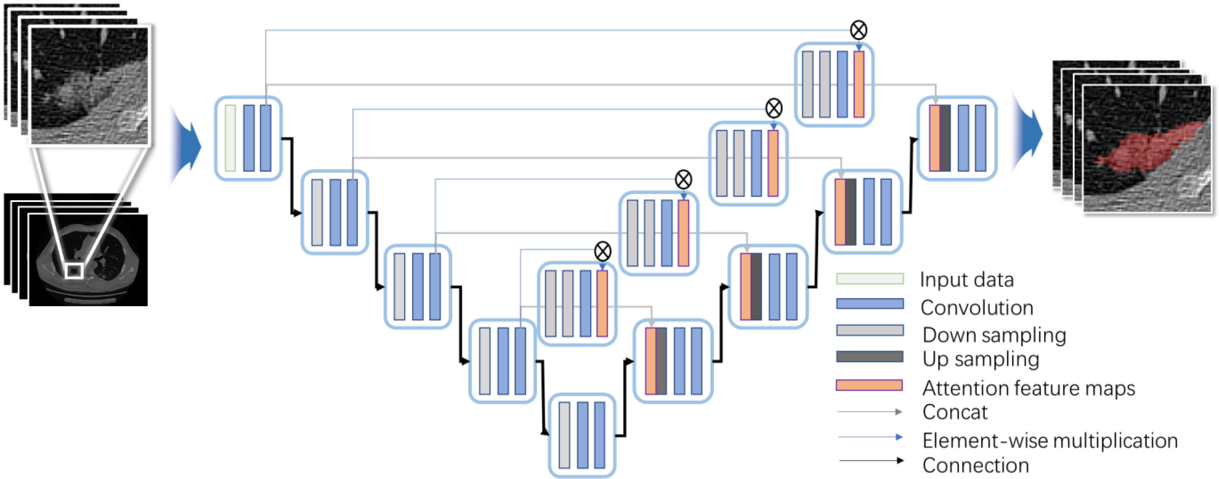
D. 3-D Attention U-Net Structure

Structure of 3-D Attention U-Net is revealed in Fig. 5. Encoder–decoder structure is retained, where the first half contains the encoding path for feature extraction and the other half uses the full-resolution segmented decoding path. In this study, four levels of structure are built to the traditional U-Net structure, and the parameters are reduced by dropout. Each level structure realizes two times 3-D convolution to extract features with the 3×3×3 kernel size, and the activation is finally completed with ReLU. In down sampling process, 3-D maximum pooling of 2×2×2 structure is performed to prevent overfitting. Therefore, number of channels doubles each time down sampling in the encoding path in turn to perform deep feature extraction accurately and effectively.

Fig. 5.

Proposed network architecture for lesion extraction.

In the decoding path, it is symmetrical with the encoding path structure to ensure that the final output matches the size of the input structure. During up-sampling, a 2×2×2 3-D upward convolution is used with a step size of 2. In each level, the 3-D convolution with the 3×3×3 kernel size is completed twice and activated by ReLU function. Along decoding path, number of feature channels is gradually reduced by half and aligned with number of encoding path channels. SoftMax function is applied to map the final 64-channel vector into two channels. The traditional U-Net [23] skip connection adopts a cascading method to realize matrix splicing. Although the feature maps are guaranteed to be uniform in size, the bottom layer information easily covers the characteristics of the high layer information. Therefore, 3-D Attention Module is used to realize skip connection, so that the information with more target features is merged into high layers, reducing the interference of the background area.

E. Binary Segmentation

The segmentation results obtained by the SoftMax activation function are a set of continuous values of [0,1]. Normally, the processing is performed by threshold segmentation. However, finding a suitable threshold is a difficult challenge, and the relationship between voxel points cannot be considered. This work utilized CRF model to obtain the corresponding binary segmentation results.

Predicted value and label are defined as and . So, CRF satisfies Gibbs distribution [25] as follow:

where energy function is expressed as

where denotes potential function, which is output by neural network, and can be expressed as

denotes binary potential function, and is expressed as

where is Potts model [26]. denotes the distance voxels and expresses grayscale difference. and are the weights that adjust the impact of paired items. Binary potential function combines relationship between space and gray, taking into account global association between pixels. Therefore, CRF can make voxels divided correctly as far as possible on boundary.

F. Combination Loss Function

The assessment of segmentation results requires to verify the overlap rate of voxels. Therefore, the training direction of the network should be to maximize the spatial overlap between the predicted results and the standard results. Dice Similarity Coefficient (DSC) is an important metrics to represent the spatial overlap rate on the images. The dice loss proposed by Soomro et al. [27] makes the network parameters to be trained in the direction of decreasing DSC value. It is defined as follows:

where is ground truth, and is the prediction result, which represents heat maps in the range of [0,1] is the matrix multiplication element by element. Finally, is a parameter, usually a small value, in case the denominator is 0 and the calculation is wrong. The value of the dice loss is obtained from

It has been proved that dice loss makes the training results unreliable in the gradient problem [28]. In the experiments of this work, dice loss usually causes the results to be not converged. In addition, Binary cross-entropy loss can avoid the problem that learning rate reduced during gradient descending. Since the learning rate can be controlled by the output error. is defined as

In order to combine the improved training direction of DSC and the advantages of stable learning rate, the work composes two loss values through the weighting factors and combination loss is defined as follows:

where and are their respective weights, and their sum is 1. By combining, new loss is established.

III. Results and Discussion

A. Data

This work tested the proposed method in private dataset and public dataset. Private dataset concluded 89 data infected with COVID-19 and were obtained from the Fifth Medical Center of the PLA General Hospital. All patients were scanned with LightSpeed VCT CT64 scanner from entrance of chest cavity to posterior costal angle. Scanning parameters were set as 120 kV voltage, 40–250 mA automatic current, 25 noise index, and 0.984:1 pitch. All CT slice thickness were 0.625 mm. Three medical experts were involved in the identification and labeling of lesion area as ground truth, where 45 data were applied for training and 44 left were utilized for testing. Some comparative and ablation experiments were established based on private dataset to test the consistency of this work. On the other hand, the public dataset established by Fan et al. [18] were applied in this work. Based on their work, 1700 data are divided into 1650 training and 50 testing. Public dataset was used to test the performance of this work by comparing other popular methods.

B. Crop Size

Limited by the calculation, the current methods of medical images processing are mainly based on 2-D network model. Usually, it is difficult to perform well with a 2-D network structure. This is because infected area of COVID-19 is multilayer continuous, containing 3-D structure. Thus, data crop is performed during ROI extraction to realize a 3-D feature network structure. Also, 64×64×64 voxels are selected as crop size for following reasons:

• 1)64×64×64 size structure satisfies , which is consistent with 512×512 slice size in space ratio. Therefore, the extracted cropping voxels occupy the same computing pressure as the 2-D network model and can satisfy the 3-D feature extraction without increasing calculation and storage burden.
• 2)Most of lung lesions are generally covered by 64 voxels. Thus, the edge information of them can be retained by these voxels.
• 3)64×64×64 voxels conform the binary structure in X-axis, Y-axis, and Z-axis. Thus, no extra interpolation operations are required during convolution, pooling, and upsampling.

C. Initialization

In order to quantify the segmentation with ground truth, four indexes were applied in the work: TP, TN, FP, and FN represent true values, true negative values, false positive values, and false negative values. They represent relationship between predicted value and true value. Based on TP, TN, FP, and FN, some metrics are defined as follows: Accuracy (ACC), Precision (PRE), Recall (REC) [29], and DSC [30]. They are expressed as

where DSC is different from dice loss. The dice loss is calculated by heat maps, which are continuous values between [0,1].

Ablation experiments were designed to verify the effect of 3-D Attention module. U-Net network model was built as a basic structure. Based on it, the model was expanded into three dimensions, and the input data were converted from the slices to voxels. Then, the combination of spatial attention and channel attention was applied as an improvement in the cascade parts of 3-D U-Net model. Finally, the attention module was converted to 3-D Attention module, and 3-D Attention U-Net was built. All network training used four samples of a small batch, Adam optimizer [31], batch normalization, normal distribution initialization, and deep supervision. The epoch was 1000, and the size of epoch was further discussed.

Fig. 6 shows results of three randomly selected segmentation come from 3-D Attention U-Net, which were obtained when the epoch was 200, 500, and 1000, respectively. Because the loss is already below 0.1, 200 epochs are an effective choice. Thus, some discussions were made by 200 epochs. Also, as epoch increases, DSC is still increasing by a small degree. If the calculation is sufficient (1000 epochs), more accurate results can be got by increasing epoch. Table I shows the results of ablation experiments. Comparing with the segmentation results of U-Net and 3-D U-Net model, 3-D U-Net network structure achieved higher ACC (93.75%). Thus, 3-D structure can learn more texture information of lung lesions and perform well than 2-D structure. In all ablation experiments, the proposed method obtained the highest accuracy (94.43%), which proved effectiveness of the proposed module. Notably, 3-D Attention U-Net reached a smaller REC. This is because the other models get more TP value than 3-D Attention U-Net, which may have a high probability lead to an oversegmentation. In terms of attention structure, the strategy of Woo et al.'s [24] attention module is to obtain the target weight of slices on each channel and each channel. The 3-D Attention Module retains the depth information, so the feature maps have more feature information.

Fig. 6.

Segmentation results of 3-D Attention U-Net, where, 1, 2, and 3 represent three different data. (a), (b), and (c) are obtained when epoch is 200, 500, and 1000. (d) is the ground truth.

TABLE I. Performance of Experiments on Private Data (Mean ± Standard Deviation).

Method	ACC	PRE	REC	DSC
U-Net [ 32 ]	93.64±8.11	68.27±21.87	98.29±1.56	57.18±18.41
3-D U- Net [ 23 ]	93.75±8.86	72.58±16.62	98.38±1.82	61.43±17.26
Attention U-Net [ 24 ]	92.39±8.39	54.45±19.83	97.53±2.15	44.12±17.24
Semi-Inf-Net_resnet	66.84±8.31	34.20±20.27	73.65±8.25	36.31±14.40
Semi-Inf-Net_res2net	56.90±7.17	22.08±14.77	64.58±5.80	23.52±11.85
Semi-Ing-Net_vgg	65.99±4.59	36.73±19.05	64.99±5.90	45.10±16.45
The proposed method	94.43±6.35	65.17±18.88	96.33±4.46	66.06±15.13

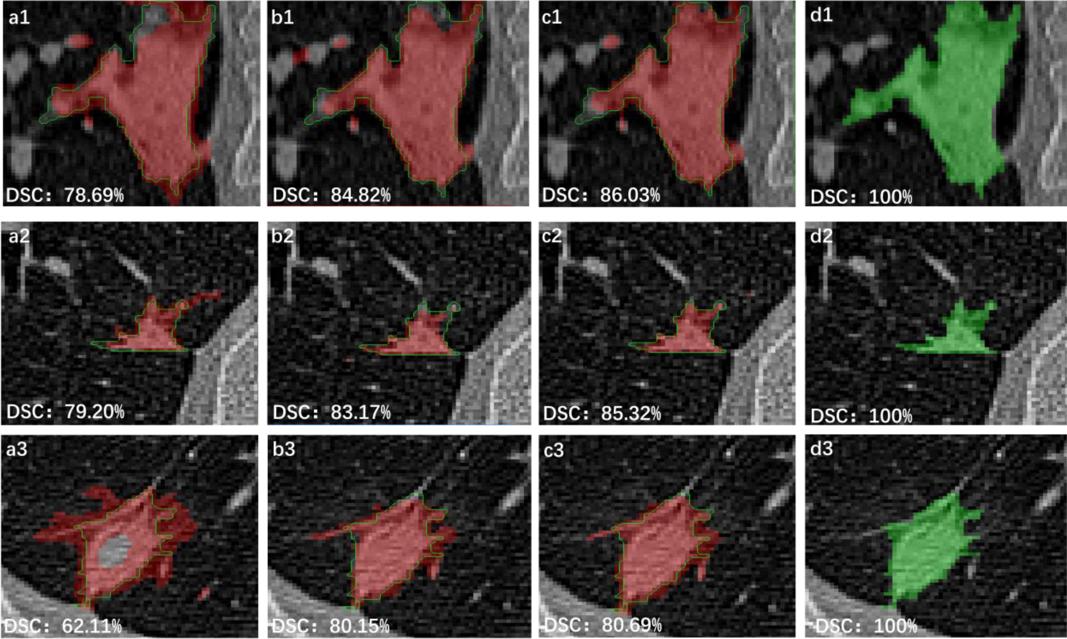
Eight datasets were selected randomly to show the segmentation results of U-Net, 3-D U-Net, and 3-D Attention U-Net in Fig. 7, where green curve shows the ground truth, red curve is the processing results of 3-D Attention U-Net, white curve represents the processing results of 3-D U-Net, and yellow curve reveals the processing results of U-Net. In all curves, red curve is the closest to the ground truth. The 3-D Attention model shows more lesion contours when cascading low-dimensional features and contains more comprehensive information when fusing features. Thus, 3-D Attention U-Net ultimately performs better.

Fig. 7.

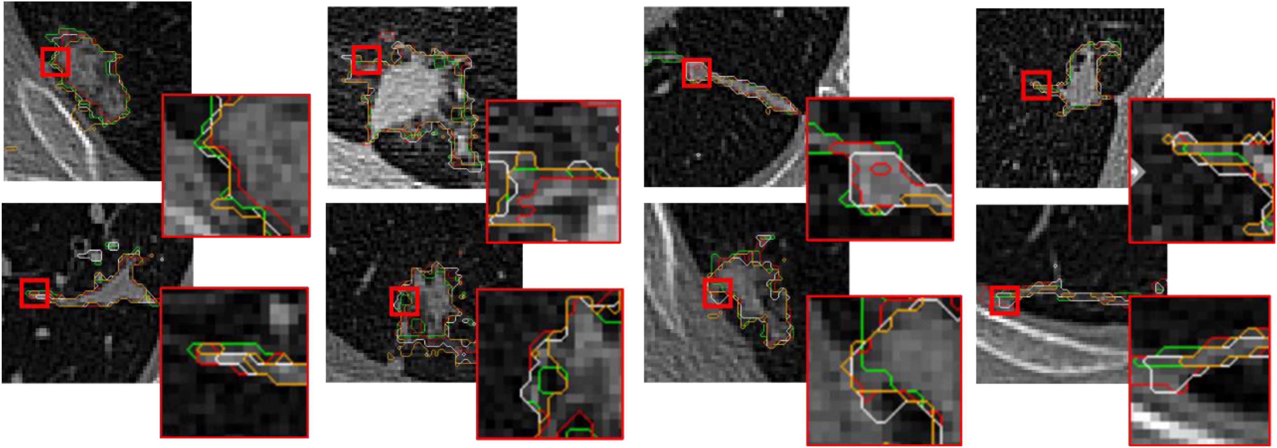
Performance of 8 data with different methods, where green is ground truth, red represents the processing results of 3-D Attention U-Net, white coms from 3-D U-Net, and yellow is obtained from U-Net.

In addition, to assess 3-D Attention Module, four datasets were randomly selected to extract the first-level cascading feature maps under 3-D U-Net and 3-D Attention U-Net. Also, an instance of them was extracted all feature maps of four levels. All feature maps were shown in Fig. 8, where a1–a4 and b1–b4 represent the feature maps extracted by 3-D Attention U-Net and 3-D U-Net, respectively. It can be seen that lesion area has more boundary contour information in 3-D Attention model, whereas feature maps information of 3-D U-Net are relatively fuzzy and almost blend with the background. In the process of gradually increasing in dimension of 3-D U-Net network, the information obtained by feature maps gradually disappears. In contrast, level-four feature map still has a fuzzy boundary in 3-D Attention U-Net. It can be seen that 3-D Attention module gradually depicts the mask map of the target area during training. It uses the mask image and the original input feature to do dot product. Finally, the effect of background suppression and target highlighting are achieved.

Fig. 8.

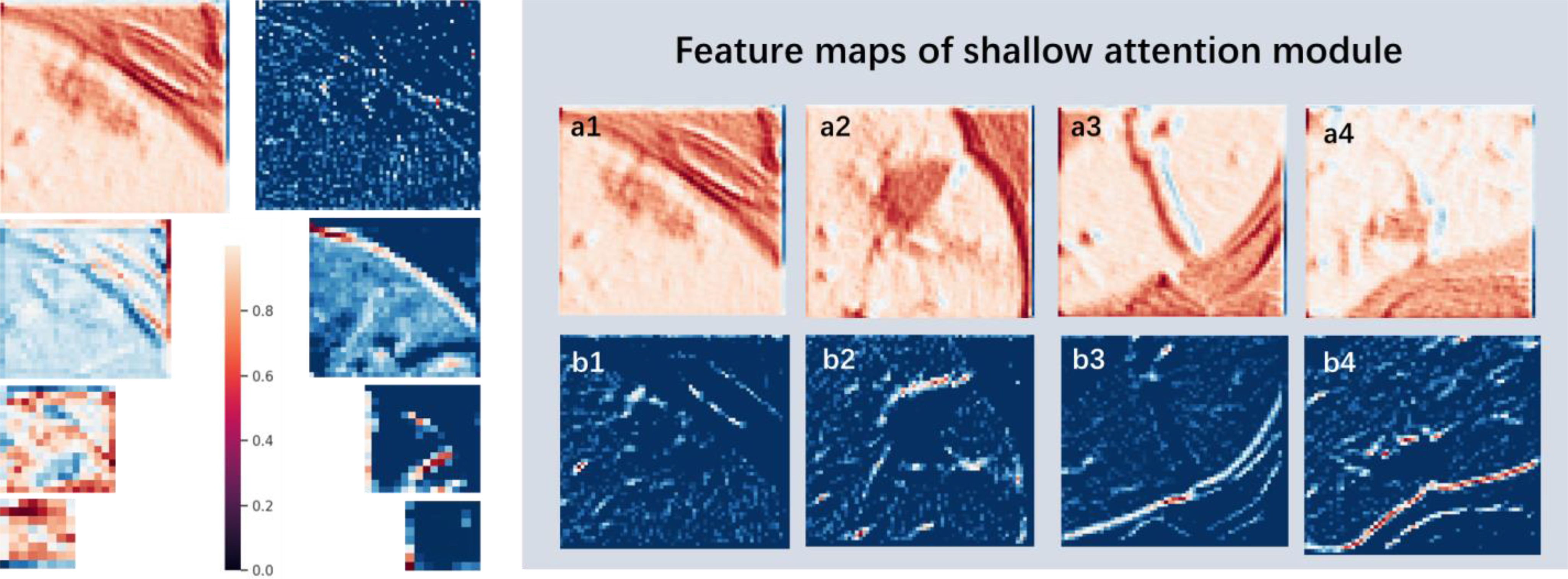
Feature maps of the attention model. The figure lists the feature maps at the cascade of the 3-D Attention model and the 3-D U-Net model; where a1 ∼ a4 represent the feature maps of the 4 sets of data at the first level of the 3-D Attention model; b1 ∼ b4 represent the corresponding 4 sets of data are featured maps at the first level of 3-D U-Net cascade.

Also, Semi-Inf-Net_resnet, Semi-Inf-Net_res2net, and Semi-Inf-Net_vgg models based on Inf-Net [18] were reestablished and trained, which are designed as the same purpose. ACC, PRE, REC, and DSC were calculated for assessments. Quantitative results were added in Table I. Because Fan et al. [18] needed to screen the slices with infected areas in advance, they could not effectively transfer to the 3-D structure. The proposed method has better performance.

D. Data Augmentation Assessment

For data augmentation, this work designed two sets of experiments for assessment. Epochs were set as 200, 500, and 1000 with 3-D Attention U-Net. One group applied data augmentation and the other group kept using original data. Fig. 9 plotted the loss, accuracy, and dice prediction of two sets experiments. Also, loss with 200, 500, and 1000 epochs were recorded. Generally, a higher loss will be obtained when data augmentation is applied for training. This is because augmentation data changes at each epoch randomly, which makes data more complicated in structure and space. Table II shows the results of these two experiments. Comparing quantitative results of two sets of experiments, although 3-D Attention U-Net with data augmentation obtained higher loss in training dataset, it achieved higher accuracy in testing dataset with 200 (61.29%), 500 (64.15%), and 1000 (66.06%) epochs. This is because data augmentation can retain the main characteristics of the original data and make dataset as diverse as possible. Finally, the models have stronger generalization ability, and their performance upper limit is improved, thereby reducing the degree of overfitting. Therefore, in a limited private database, data augmentation method is a very effective strategy.

Fig. 9.

Loss, accuracy, and dice prediction in 3-D Attention U-Net at 1000 epochs, where (a) represents results under data augmentation and (b) is obtained by original data.

TABLE II. Performance of Data Augmentation (Mean±Standard Deviation).

Method	DSC (%)	ACC (%)
Original Data (epoch = 200)	55.88±15.29	91.30±8.94
Augmented Data (epoch = 200)	61.29±16.39	93.22±6.81
Original Data (epoch = 500)	58.47±16.46	93.16±8.44
Augmented Data (epoch = 500)	64.15±16.66	94.26±7.79
Original Data (epoch = 1000)	60.26±16.87	93.44±8.03
Augmented Data (epoch = 1000)	66.06±15.13	94.43±6.35

E. Loss Function Improvement Assessment

The work tested the convergence effect of loss function. The experiments designed as: Binary cross-entropy, dice and combination loss were designed as loss in model with 3-D Attention U-Net, respectively. Also, combination loss was divided into five groups weights: [,] = [0.3, 0.7], [0.5, 0.5], [0.6, 0.4], [0.8, 0.2], [0.9, 0.1]. Loss, accuracy, and dice prediction were plotted respectively.

Table III shows combination loss with different weights. All epochs were set as 200. In the discussion of weights, the weight coefficient of [0.8, 0.2] achieved relatively better results. Thus, a deeper experiment and discussion were done. Three sets of experiments were made by 3-D Attention U-Net with different loss functions. [0.0, 1.0], [0.8, 0.2], and [1.0, 0.0] weight coefficients represented dice, combination, and binary cross-entropy loss. The epochs were 1000, in which the loss value of all networks is almost stable. Fig. 10 shows the loss, accuracy, and loss prediction of three experiments, where when the epoch is 200, the network with dice loss reaches the lowest loss 0.03527 [Fig. 10(a)]. By contrast, combination loss and binary cross-entropy loss reach the loss of 0.04821 [see Fig. 10(b)] and 0.05262 [see Fig. 10(c)]. This proves that the dice loss can balance the imbalance of positive and negative samples to a certain extent, making the network converge quickly. In addition, the dice loss stabilizes after 200 epochs. However, combination loss and binary cross-entropy loss still have an obvious downward trend. This also proves that the gradient form of dice loss in the training process is not optimal, which causes loss to easily fall to the local minimum, so the relative global optimal value cannot be obtained. Table IV shows the DSC, ACC, and PRE of the three experiments after 1000 epochs. Comparing combination loss and binary cross-entropy loss, the network with combination loss has achieved greater DSC (66.06%). This is because dice loss is more in line with the real goal of maximizing DSC segmentation during the training process, and binary cross-entropy loss has a better gradient form. and are weights to balance the training direction and gradient to a certain extent, so as to achieve better convergence efficiency and training effect. It is worth mentioning that although experiments show that [0.8, 0.2] weight has a better effect. But this is volatile. In practical applications, parameters need to be adjusted according to different datasets to balance the training effect. When the epoch is 1000, loss almost reaches the lowest value. Three sets of comparative experiments proved the feasibility of combination loss in handling of COVID-19 CT images.

TABLE III. Performance of Different Weights With Combinational Loss (Mean±Standard Deviation).

Method	DSC (%)	ACC (%)	PRE (%)
[0.3, 0.7]	58.57±16.97	92.03±9.05	53.12±18.56
[0.5, 0.5]	56.97±17.64	92.37±8.58	52.28±19.26
[0.6, 0.4]	55.67±16.46	90.85±9.73	48.43±17.89
[0.8, 0.2]	61.29±16.39	93.22±6.81	65.17±18.88
[0.9, 0.1]	57.75±17.26	92.26±6.69	51.70±21.56

Fig. 10.

Loss, accuracy, and dice prediction of 3-D Attention U-Net, where (a), (b), and (c) represent convergence curves of network with dice loss, Binary cross-entropy loss, and combination loss, respectively.

TABLE IV. Performance of Different Loss (Mean±Standard Deviation).

Method	DSC (%)	ACC (%)	PRE (%)
[0.0, 1.0]	62.21±17.96	93.22±8.73	61.25±19.82
[0.8, 0.2]	66.06±15.13	94.43±6.35	69.91±18.43
[1.0, 0.0]	62.07±16.71	93.20±8.52	61.46±19.36

F. CRF Assessment

Fig. 11 shows the probability obtained from the output layer. The main controversial position comes from the voxels of about 0.5 intensity on boundary. In this study, 0.5 threshold group and CRF method were designed to compare the segmentation results. Ten data with ACC and DSC were quantitative assessed in Table V. The results of increase magnitude with CRF were calculated in contrast to threshold. Although the performance improvement is small, it proves that CRF has important potential in dealing with boundaries and connected domains. That is because CRF obtains the relationship between pixel values by establishing a global energy field using gray value and the actual relative distance, so that the picture is segmented at the boundary as much as possible. Also, the isolated segmentation is reduced. This has certain advantages when dealing with COVID-19 infected areas with connected characteristics. In contrast, threshold segmentation can only get independent features of each pixel. Also, the strategy also avoids looking for the best threshold.

Fig. 11.

Probability map obtained from the output layer.

TABLE V. Performance of Threshold and Crf (Mean±Standard Deviation).

Data (%)	ACC (Threshold)	ACC (CRF)	DSC (Threshold)	DSC (CRF)
Data 1	98.4177	98.4207 (0.0030)	76.8035	76.8223 (0.0188)
Data 2	96.3318	96.3425 (0.0107)	80.8095	80.8539 (0.0444)
Data 3	98.5073	98.5218 (0.0145)	49.9936	50.0322 (0.0386)
Data 4	98.9464	98.9482 (0.0018)	85.3116	85.3234 (0.0118)
Data 5	98.8487	98.8518 (0.0031)	74.1078	74.1276 (0.0198)
Data 6	99.0345	99.0372 (0.0027)	74.1078	74.1276 (0.0198)
Data 7	99.1189	99.1291 (0.0102)	46.7005	46.9193 (0.2188)
Data 8	98.9582	98.9624 (0.0042)	64.6838	64.7394 (0.0556)
Data 9	95.8088	95.8317 (0.0229)	62.0497	62.1785 (0.1288)
Data 10	94.6930	94.7132 (0.0202)	62.0497	62.1785 (0.1288)

G. Performance Evaluation

This work was tested on public dataset and compared with some latest methods. Table VI shows the quantitative results of these experiments. From property of public dataset, it has achieved higher performance than private dataset. This is because the diversification of data improves the model performance. In addition, many classic models are difficult to achieve better performance, such as U-Net [32], U-Net++ [33], and DeepLab [34]. Therefore, these common networks are still challenging for COVID-19 CT images. Some networks have achieved higher REC, but the appropriate DSC index was not reached, such as Mini-Seg [19] and COVID-SegNet [20]. This may be caused by larger true negative values, which may lead to a clinical missed diagnosis. Also, the proposed method achieved the highest DSC, which means that the segmented infected area has the greatest coincidence rate with the clinician's standard. Other confirmatory metrics have also reached acceptable values. Due to the imperfection of public dataset, small sample learning is very important, such as [18] and [22]. This work solved this problem by data augmentation. In addition, it has more potential for spatial applications of 3-D structures. There are still some improvements in this article, such as improving the recognition rate of negative samples and reducing false positive values. This also provides a direction for us to improve next.

TABLE VI. Performance of Experiments on Public Data (Mean±Standard Deviation).

Method (%)	ACC	PRE	REC	DSC
U-Net [32]	86.78±9.88	57.59±19.67	90.64±10.73	55.69±16.91
U-Net++ [33]	86.92±7.30	50.16±19.43	85.23±9.06	62.34±18.68
DeepLab [34]	82.89±5.29	62.83±7.12	87.49±6.05	43.93±7.58
DI-U-Net [35]	90.67±6.80	61.93±18.88	90.99±7.70	69.54±16.63
Dense U-Net [35]	92.79±4.49	69.80±12.51	93.93±4.88	73.60±11.31
Inf-Net [18]	89.51±6.93	58.90±14.44	87.95±9.01	69.88±12.58
Semi-Inf-Net [18]	92.01±4.71	65.74±12.96	91.46±6.35	74.11±10.87
Mini-Seg [19]	87.53±8.24	56.42±8.73	97.64±3.56	55.97±7.73
COVID-SegNet [20]	86.79±5.09	57.80±12.14	91.52±4.50	50.01±7.98
TV-UNet [21]	92.34±4.78	67.94±12.06	93.67±4.66	72.94±10.60
Proposed Method	93.92±3.87	78.26±9.94	96.39±2.92	75.22±11.25

IV. Conclusion

The work proposed an automatic method applied to lung lesions segmentation of COVID-19 from CT Images. Proposed ROI extraction was applied to focus on lung lesions. Also, data augmentation and combination loss were applied to improve the training effect. Despite the presence of unclear boundaries in the infected area, morphological changes, and poor contrast with the vascular tissue, 3-D Attention Module can focus on boundary contour information. Thus, the network can learn more details of target area. In postprocessing, the applied CRF can pay attention to the correlation of each voxel point to improve the accuracy of voxel point classification near boundary.

The proposed method was compared with some common models and other algorithms designed for COVID-19 segmentation. Also, DSC, ACC, PRE, and REC were applied as assessment metrics. The results show that this work has higher performance in the private dataset and the public dataset. In addition, discussions on data augmentation, epoch, loss function, and CRF were conducted to verify their effectiveness. Due to the similarity of case structures, the proposed model also has certain potential in other physiological parts, such as lung nodules and liver lesions. Code of this work has been released at: https://github.com/USTB-MedAI/3DAttUnet.

Biographies

Cheng Chen was born in Sichuan, China, in July 1994. He received the B.S. degree in electronic information engineering from the School of Computer and Communication Engineering, University of Science and Technology Beijing, China, in June 2017. He is currently working toward the Ph.D. degree in communication and information engineering from the School of Computer and Communication Engineering, University of Science and Technology Beijing, in September 2017.

His main research directions are medical image processing, medical artificial intelligence (especially machine learning and deep learning), three-dimensional reconstruction and visualization, speech signal processing, and augmented reality navigation.

Kangneng Zhou was born in Zhejiang, China, in December 1997. He received the B.S. degree in Internet of Things from the School of Computer & Communication Engineering, University of Science and Technology Beijing, Beijing, China, in June 2020. He is currently working toward the M.S. degree in computer science and technology from the School of Computer & Communication Engineering, University of Science and Technology Beijing.

His main research directions are machine learning (especially deep neural networks), generative adversarial networks, variational autoencoder, and generative flow. He also has a keen interest in medical image processing, 3-D reconstruction and other areas.

Muxi Zha was born in Hunan, China, in November 1998. She received the B.E. degree in communication engineering from the School of Computer & Communication Engineering, University of Science and Technology Beijing, Beijing, China, in June 2020. She is currently working toward the M.E. degree in electronic information from the College of Electrical and Information Engineering, Hunan University, Changsha, China.

Her main research interests are computer vision and image processing including traditional and deep learning methods, especially object detection, and arbitrarily-oriented, curved, or deformed texts recognition under natural scene. She also have interests in 3-D reconstruction and other areas.

Xiangyan Qu was born in Henan, China, in September 1999. He is also going to be a Ph.D. Student with the Institute of Information Engineering (IIE), Chinese Academy of Sciences (CAS) supervised by Prof. Jing Yu. He is currently a senior student with the University of Science and Technology Beijing (USTB), China. His major is Internet of Things Engineering in the School of Computer and Communication Engineering.

His primary research interests include multimodal machine learning. Specifically, his current research focuses on cross-modal retrieval, e.g., visual question answering, video question answering, visual dialog, image captioning, video captioning, and visual grounding.

Xiaoyu Guo was born in Henan, China, January 1991. He received the B.S. degree in electronic information engineering from Zhengzhou University, Zhengzhou, China, in 2013. He is currently working toward the Ph.D. degree with the School of Computer & Communication Engineering, University of Science and Technology Beijing, Beijing, China. His major is communication and information systems.

His research interests include medical image processing and application of artificial intelligence in medical images. He has published several papers on automatic vessel segmentation. He is working on combing 2-D and 3-D image processing methods to improve the performance of deep learning method in medical images.

Hongyu Chen was born in Shandong, China, in May 1997. He received the B.S. degree in network engineering from the School of Computer and Control Engineering, North University of China, China, in June 2020. He is currently working toward the M.S. degree with the School of Computer and Communication Engineering, University of Science and Technology Beijing, Beijing, China.

His main research directions are machine learning and deep learning (especially medical image processing and medical artificial intelligence). He is also interested in recommendation systems (collaborative filtering, content-based filtering, cold start problem and so on) and text mining (opinion mining, search, text summarization and so on).

Zhiliang Wang received the M.S. degree from Yanshan University, Qinhuangdao, China, in 1982, and the Ph.D. degree from the Harbin Institute of Technology, Harbin, China, in 1989, both in control theory and control engineering.

He is currently a Professor and the Doctorate Supervisor with the School of Computer and Communication Engineering, University of Science and Technology, Beijing, China. His research interests include security control of cyber-physical systems and active industrial control systems, and theory and application of networked control systems, and artificial intelligence.

Dr. Wang is a Senior Board Member of the Chinese Association of Artificial Intelligence and the Director of the Beijing Society of Internet of Things.

Ruoxiu Xiao received the Ph.D. degree in optical engineering from the Beijing Institute of Technology, Beijing, China, in 2014.

He was a Postdoctoral Research Fellow with the School of Medicine, Tsinghua University, China. He was previously a Visiting Research Scholar with the Stanford Medicine, Stanford University, CA, USA, from 2018 to 2019. He is currently an Associate Professor and Master Director with the School of Computer and Communication Engineering, University of Science and Technology Beijing, Beijing. His main research interests include medical image processing, computer aided surgery, and machine learning and pattern recognition.

Dr. Xiao is also the Member of China Association for Disaster & Emergency Rescue Medicine.

Funding Statement

This work was supported in part by National Natural Science Foundation of China under Grant 61701022, in part by National Key Research and Development Program (2017YFB1002804, 2017YFB1401203), in part by Beijing Natural Science Foundation (7182158), in part by Fundamental Research Funds for the Central Universities (FRF-DF-20-05), and in part by the Beijing Top Discipline for Artificial Intelligent Science and Engineering, University of Science and Technology Beijing.

References

- [1].Johns Hopkins University, “COVID-19 dashboard,” Jan. 2021. [Online]. Available: https://coronavirus.jhu.edu/map.html
- [2].Ai T. et al. , “Correlation of chest CT and RT-PCR testing in coronavirus disease 2019 (COVID-19) in China: A report of 1014 cases,” Radiology, vol. 296, no. 2, pp. E32–E40, Feb. 2020. [DOI] [PMC free article] [PubMed] [Google Scholar]
- [3].Chung M. et al. , “CT imaging features of 2019 novel coronavirus (2019-nCoV),” Radiology, vol. 295, no. 1, pp. 202–207, Feb. 2020. [DOI] [PMC free article] [PubMed] [Google Scholar]
- [4].Ng M. Y. et al. , “Imaging profile of the COVID-19 infection: Radiologic findings and literature review,” Radiol., Cardiothorac Imag., vol. 2, no. 1, Feb. 2020, Art. no. e200034. [DOI] [PMC free article] [PubMed] [Google Scholar]
- [5].Song F. X. et al. , “Emerging 2019 novel coronavirus (2019-nCoV) pneumonia,” Radiology, vol. 295, no. 1, pp. 210–217, Feb. 2020. [DOI] [PMC free article] [PubMed] [Google Scholar]
- [6].Rubin G. D. et al. , “The role of chest imaging in patient management during the COVID-19 pandemic: A multinational consensus statement from the Fleischner society,” Chest, vol. 158, no. 1, pp. 106–116, Jul. 2020. [DOI] [PMC free article] [PubMed] [Google Scholar]
- [7].Li X. et al. , “CT imaging changes of corona virus disease 2019 (COVID-19): A multi-center study in Southwest China,” J. Transl. Med., vol. 18, no. 1, Apr. 2020, Art. no. 154. [DOI] [PMC free article] [PubMed] [Google Scholar]
- [8].Babiker M. S., “COVID-19 CT features: A scoping literature review,” Scholar J. Appl. Med. Sci., vol. 8, no. 8, pp. 1802–1808, Aug. 2020. [Google Scholar]
- [9].Kovacs A., Palasti P., Vereb D., Bozsik B., Palko A., and Kincses Z. T., “The sensitivity and specificity of chest CT in the diagnosis of COVID-19,” Eur. Radiol., Oct. 2020, doi: 10.1007/s00330-020-07347-x. [DOI] [PMC free article] [PubMed]
- [10].Cobes N. et al. , “Ventilation/perfusion SPECT/CT findings in different lung lesions associated with COVID-19: A case series,” Eur. J. Nucl. Med. Mol. Imag., vol. 47, no. 10, pp. 2453–2460, Sep. 2020. [DOI] [PMC free article] [PubMed] [Google Scholar]
- [11].Consultant M. S. and Anaesthesiology R. G.. “COVID-19 pandemic: A multifaceted challenge for science and healthcare,” Trends Anaesth. Crit. Care, vol. 34, pp. 1–3. Oct. 2020. [DOI] [PMC free article] [PubMed] [Google Scholar]
- [12].Ferrer R., “COVID-19 pandemic: The greatest challenge in the history of critical care,” Medicina Intensiva (English Ed.), vol. 44, no. 44, pp. 323–324, Aug. 2020. [DOI] [PMC free article] [PubMed] [Google Scholar]
- [13].Abdel-Basset M., Chang V., and Mohamed R., “HSMA_WOA: A hybrid novel slime mould algorithm with whale optimization algorithm for tackling the image segmentation problem of chest X-ray images,” Appl. Soft Comput., vol. 95, Oct. 2020, Art. no. 106642. [Online]. Available: 10.1016/j.asoc.2020.106642 [DOI] [PMC free article] [PubMed] [Google Scholar]
- [14].Chen C. et al. , “Pathological lung segmentation in chest CT images based on improved random walker,” Comput. Methods Programs Biomed., Nov. 2020. [Online]. Available: 10.1016/j.cmpb.2020.105864 [DOI] [PubMed]
- [15].Huang Q., Sun J. F., Ding H., Wang X. D., and Wang G. Z., “Robust liver vessel extraction using 3D U-Net with variant dice loss function,” Comput. Biol. Med., vol. 101, no. 1, pp. 153–162, Oct. 2018. [DOI] [PubMed] [Google Scholar]
- [16].Lal A., Mishra A. K., and Sahu K. K., “CT chest findings in coronavirus disease-19 (COVID-19),” J. Formosan Med. Assoc., vol. 119, no. 5, pp. 1000–1001, May 2020. [DOI] [PMC free article] [PubMed] [Google Scholar]
- [17].Li X., Pan Z., Xia Z., Li R., and Li H., “Clinical and CT characteristics indicating timely radiological reexamination in patients with COVID-19: A retrospective study in Beijing, China,” Radiol. Infect. Dis., vol. 7, no. 2, pp. 62–70, Jun. 2020. [DOI] [PMC free article] [PubMed] [Google Scholar]
- [18].Fan D. P. et al. , “Inf-Net: Automatic COVID-19 lung infection segmentation from CT scans,” IEEE Trans. Med. Imag., vol. 39, no. 8, pp. 2626–2637, May 2020. [DOI] [PubMed] [Google Scholar]
- [19].Qiu Y., Liu Y., and Xu J., “MiniSeg: An extremely minimum network for efficient COVID-19 segmentation,” 2020, arXiv:2004.09750v2. [DOI] [PubMed]
- [20].Yan Q. S. et al. , “COVID-19 chest CT image segmentation–A deep convolutional neural network solution,” Aug. 2020, arXiv:2004.10987v2.
- [21].Saeedizadeh N., Minaee S., Kafieh R., Yazdani S., and Sonka M., “COVID TV-UNet: Segmenting COVID-19 chest CT images using connectivity imposed U-Net,” Aug. 2020, arXiv:2007.12303v3. [DOI] [PMC free article] [PubMed] [Google Scholar]
- [22].Abdel-Basset M., Chang V., Hawash H., Chakrabortty R. K., and Ryan M., “FSS-2019-nCov: A deep learning architecture for semi-supervised few-shot segmentation of COVID-19 infection,” Knowl.-Based Syst., vol. 215, Jan. 2021, Art. no. 106647. [Online]. Available: 10.1016/j.knosys.2020.106647 [DOI] [PMC free article] [PubMed] [Google Scholar]
- [23].Çiçek O., Abdulkadir A., Lienkamp S. S., Brox T., and Ronneberger O., “3D U-Net: Learning dense volumetric segmentation from sparse annotation,” in Proc. Med. Imag. Comput. Comput. Assisted Intervention Soc., 2016, pp. 424–432. [Google Scholar]
- [24].Woo S., Park J., Lee J. Y., and Kweon I. S., “CBAM: Convolutional block attention module,” in Proc. Eur. Conf. Comput. Vision, 2018, pp. 3–19. [Google Scholar]
- [25].Guo M. and Gursoy M. C., “Gibbs distribution based antenna splitting and user scheduling in full duplex massive MIMO systems,” IEEE Trans. Veh. Technol., vol. 69, no. 4, pp. 4508–4515, Apr. 2020. [Google Scholar]
- [26].Davies E., “Counting proper colourings in pp. 4.-Regular graphs via the potts model,” Electron. J. Combinatorics, vol. 25, 2018, Art. no. P4.7, doi: 10.37236/7743. [DOI] [Google Scholar]
- [27].Soomro T. A., Afifi A. J., Gao J., Hellwich O., Paul M., and Zheng L., “Strided U-Net model: Retinal vessels segmentation using dice loss,” in Proc. Digital Image Comput., Techn. Appl., 2018,. pp. 1–8. [Google Scholar]
- [28].Mehrtash A., Wells W. M., Tempany C. M., Abolmaesumi P., and Kapur T., “Confidence calibration and predictive uncertainty estimation for deep medical image segmentation,” IEEE Trans. Med. Imag., vol. 39, no. 12, pp. 3868–3878, Dec. 2020. [DOI] [PMC free article] [PubMed] [Google Scholar]
- [29].Xiao R. X., Ding H., Zhai F. W., Zhao T., Zhou W. J., and Wang G. Z., “Vascular segmentation of head phase-contrast magnetic resonance angiograms using grayscale and shape features,” Comput. Methods Programs Biomed., vol. 142, pp. 157–4166, Apr. 2017. [DOI] [PubMed] [Google Scholar]
- [30].Li G. D., Chen X. J., Shi F., Zhu W. F., Tian J., and Xiang D. H., “Automatic liver segmentation based on shape constraints and deformable graph cut in CT images,” IEEE Trans. Image Process., vol. 24, no. 12, pp. 5315–5329, Sep. 2015. [DOI] [PubMed] [Google Scholar]
- [31].Bock S., Goppold J., and Weis M., “An improvement of the convergence proof of the ADAM-Optimizer,” in Proc. Ostbayerische Technische Hochschule Regensburg, 2018, pp. 80–84. [Google Scholar]
- [32].Ronneberger O., Fischer P., and Brox T., “U-Net: Convolutional networks for biomedical image segmentation,” in Proc. Med. Imag. Comput. Comput. Assisted Intervention Soc., 2015, pp. 234–241. [Google Scholar]
- [33].Zhou Z., Siddiquee M. R., Tajbakhsh N., and Liang J., “UNet++: A nested U-Net architecture for medical image segmentation,” in Proc. Int. Workshop Deep Learn. Med. Image Anal., 2018, pp. 3–11. [DOI] [PMC free article] [PubMed] [Google Scholar]
- [34].Chen L., Papandreou G., Schroff F., and Adam H., “Rethinking atrous convolution for semantic image segmentation,” 2017, arXiv:1706.05587. [Google Scholar]
- [35].Guo X. et al. , “Retinal vessel segmentation combined with generative adversarial networks and dense U-Net,” IEEE Access, vol. 8, pp. 194551–194560, Oct. 2020. [Google Scholar]