Integration of CNN, CBMIR, and Visualization Techniques for Diagnosis and Quantification of Covid-19 Disease

Abstract

Diagnosis techniques based on medical image modalities have higher sensitivities compared to conventional RT-PCT tests. We propose two methods for diagnosing COVID-19 disease using X-ray images and differentiating it from viral pneumonia. The diagnosis section is based on deep neural networks, and the discriminating uses an image retrieval approach. Both units were trained by healthy, pneumonia, and COVID-19 images. In COVID-19 patients, the maximum intensity projection of the lung CT is visualized to a physician, and the CT Involvement Score is calculated. The performance of the CNN and image retrieval algorithms were improved by transfer learning and hashing functions. We achieved an accuracy of 97% and an overall prec@10 of 87%, respectively, concerning the CNN and the retrieval methods.

I. Introduction

The most common approach for the diagnosis of COVID-19 disease is the Reverse Transcription-Polymerase Chain Reaction (RT-PCR) with clinical symptoms [1]. The method has some restrictions, including the limited number of the corresponding kits, its low sensitivity, repeatability, and the process's stability in different sampling conditions. Sometimes, one has to repeat the test several times before the final confirmation of the results [2]. However, medical imaging is a replacement for diagnostic kits.

Chest X-ray and Computed Tomography (CT) scan images are widely used in the diagnosis of the Coronavirus disease (COVID-19); however, automatic fulfillment of the task is an emerging field in medical image processing [3]–[6]. The transparency of a COVID-19 infected lung is changed in X-ray/CT images, and some Ground Glass Opacities (GGOs) are seen as well [7]. The thickening of some pulmonary vessels is the other symptom. Compared to laboratory tests, imaging techniques have higher sensitivity and True Positive (TP) rates, and they are prepared more quickly. Moreover, they can reveal the illness even in its initial stages [2], [8], [9]. More on the significance of imaging approaches are found in [10]–[13].

II. Related Works

The research on COVID-19 detection using X-ray images can be classified into two groups. (1) Some researchers evaluated the performance of available deep architectures, including ResNet50 and ResNetV2, to obtain the best achievement. [14], [3]. (2) Others developed their proprietary architectures [6], [4], [15], [8]. Almost all these methods used the transfer learning technique to compensate for the small amount of available data. Nearly half of the researches discriminated between healthy and COVID-19 X-ray images [14], [3], [4], [16] while others considered viral/bacterial pneumonia, severe acute respiratory syndrome (SARS), and other lung diseases [8], [6], [15], [17].

Mohammadi et al. employed several pre-trained networks to differentiate between COVID-19 and healthy X-ray images [14]. They achieved 99% accuracy; however, they did not discriminate between viral pneumonia and COVID-19, which show similar signs in the X-ray images. Narin et al. compared three available network architectures, including ResNet50, InceptionV3, and Inception-ResNetV2 models, to differentiate between health y and COIVD-19 [3]. They concluded that a ResNet50 pre-trained model obtained the best performance with an accuracy of 98% among other architectures. Zhang et al. differentiated between pneumonia and COVID-19 datasets using a proprietary architecture [6]. Wang et al. used COVIDNet, a proprietary network, to detect Coronavirus disease [4]. To solve for the low number of data, they suggested a data generation algorithm to prepare 16756 synthesized data and called them CovidX. Khan et al. tailored an already developed model, Xception, to differentiate between healthy, pneumonia, and COVID-19 X-ray images [15]. Che Azemin used ResNet-101 to distinguish COVID-19 cases [16]. Unlike previous methods, the work presented by Jian et al. is a distinct innovation [17]. They proposed a two-step architecture consisting of two deep neural networks. In the first step, they classified input data into normal, bacterial pneumonia, and viral pneumonia. The second stage labeled viral data as COVID-19 and others. This two-step classification achieved the best performance among similar studies. Finally, Ghoshal et al. addressed uncertainty in the classification of X-ray images [5].

Most of the above researches used available techniques to detect COVID-19. The problem overlooked in these researches is designing an algorithm that complies with the limitation of the specific situation, including the low number of available data, the disease's similarity to some other pulmonary illnesses, and the explainability issue of deep neural networks. As solutions for data shortage and similarity of COVID-19 to other pulmonary diseases, we propose two main novelty to our CNN training method: (1) two-stage domain adaptation, (2) incremental knowledge transfer. We take advantage of the low-level features available in the pre-trained networks and add extra knowledge about the high-level features of the domain of X-ray images. This form of domain adaptation is performed in two stages: Once with more available X-ray images of the Normal-Pneumonia dataset on the pre-trained network, then, using fewer data of the COVID19-Normal-Pneumonia dataset on the fine-tuned model of the previous stage. Both of the above steps gradually transfer knowledge to the model and eliminate the risk of overfitting. In the incremental knowledge transfer, first, we regulate the end layers of the pre-trained network (in which the weights would correspond to the high-level features), then we include more layers and continue the training.

To develop an explainable deep neural network, we propose a decision support system to give a physician an appropriate insight into CNN's result. It includes an image retrieval component to fetch similar images and a visualization unit to quantify the disease's extent. As far as we know, there is no research to use Content-Based Image Retrieval techniques as a medical consultation system to detect coronavirus infection. Moreover, the employed visualization techniques, together with the CT involvement scores calculation, have been performed for the first time based on our knowledge.

III. Materials and Methods

A. Datasets

The available dataset consists of two chest X-rays and one set of CT images. The first data belongs to Kaggle's Chest X-ray Images (Pneumonia) [18] containing healthy and pneumonia cases. We used the COVID19 dataset curated by J. Cohen [19] as the second dataset. Specifications of the training and test sets are in Table I. For the CNN model, we prepared two sets of images from the datasets. The first set which was used the Normal-Pneumonia (NP) phase contained 1000 training and 100 test images from each class, all from the Kaggle's dataset. In the Covid19-Normal-Pneumonia (CNP) phase, we used an extra 200 training and 100 test images from Normal and Pneumonia classes in the Kaggle's dataset and 110 training and 100 test images obtained from J. Cohen's COVID-19 dataset.

TABLE I. Number of the Training and Test Sets.

Algorithm	Dataset	Healthy	Pneumonia	COIVD-19
The CNN Model	Kaggle's (Training)	1200	1200	–
	Kaggle's (Test)	200	200	–
	Cohen's (Training)	–	–	110
	Cohen's (Test)	–	–	100
The CBMIR	Kaggle's (Training)	1211	1207	–
	Kaggle's (Test)	134	134	–
	Cohen's (Training)	–	–	197
	Cohen's (Test)	–	–	22

Concerning CT data, we used ten public volumes from the COVID-19 image collection [19]. The size of the images was 200-301 × 512 × 512, the inter-slice resolution was 0.6836 × 0.6836 to 0.8105 × 0.8105 mm², and the slice thickness was 1–1.5 mm.

B. Methods

1). Overview of the Method

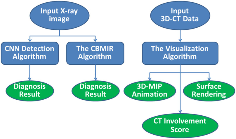
The proposed decision support system consists of three modules (Fig. 1). First, a CNN-based infection diagnosis uses deep neural networks to differentiate between COVID-19, healthy, and pneumonia cases. The remaining modules give interpretation support to the results of the CNN. They consist of a system retrieving similar images from an atlas of X-ray data and quantification and visualization modules that evaluates the percentage of the GGOs in an infected lung and displays their locations.

Fig. 1.

The overview of the proposed framework.

The proposed system accepts an X-ray of a patient as input data. Then, a Convolutional Neural Network (CNN) calculates the probability of the infection by the coronavirus. Moreover, a Content-Based Medical Image retrieval (CBMIR) algorithm retrieves similar images and labels the input test image. Both the CNN and the CBMIR algorithms distinguish between healthy, COVID-19, and viral pneumonia infected cases. If the patient is diagnosed with Corona, segmentation of the abnormalities and lung lobes of the corresponding CT image are performed, the CT Involvement Score is calculated, and the location of the lung lobes, GGOs, and vasculatures are represented in 3D view.

We implemented the proposed algorithms using Python, the TensorFlow [20] framework, MATLAB, C++, and VTK toolkit [21]. A personal computer running MS Windows 10 was used with Intel Core i5-7500 CPU, 16 GB RAM, and a GeForce GTX 1070Ti graphics card. The CNN codes were performed on the graphics processing unit (GPU).

2). The CNN Model

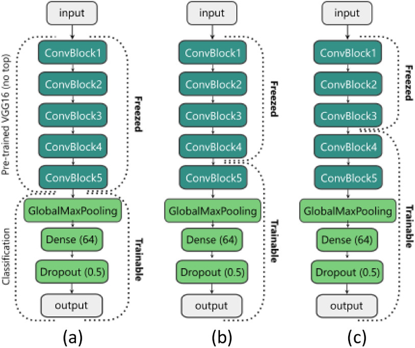
The architecture of the proposed CNN model is illustrated in Fig. 2. We use the VGG16 [22] model that is pre-trained on the ImageNet [23] dataset without the Dense (Fully-connected) layers. Therefore, our pre-trained VGG16 (which we call the ‘base model’) is made up of five Convolutional (Conv) blocks. Each block has two or three Conv layers that end with a Max-pooling layer. We replace the Dense layers of the VGG16 with our classification layers (Fig. 2). Our classification front consists of a Global Max-pooling layer, a Dense layer with 64 units and the Rectified Linear Unit (ReLU) activation function, a Dropout layer with a rate of 50%, and finally a Dense layer (output layer in Fig. 2) with two or three units (based on the number of the classes) with the Softmax activation function. We have also tried other available pre-trained models like the InceptionV3 [24], DenseNet [25], or ResNet [26] for the base model, but all of them led to overfitting.

Fig. 2.

Training stages of the proposed model. (a) Only the classification front is trained. (b) The last ConvBlock of the base model and the classification head are trained (c) The two last ConvBlocks of the base model and the classification head are trained.

Our incremental domain adaptation and knowledge transfer method have two main phases. The first phase is called the NP Phase, in which we train our model on the NP (Normal- Pneumonia) dataset to learn the domain of the chest X-ray images. The second phase is called the CNP (COVID19-Normal- Pneumonia) Phase, in which we use the trained model of the previous stage and fine-tune it using the CNP dataset.

Both phases have two steps; one step is the warm-up in which we freeze most layers of the base model and train our classification layers. The second step acts as fine-tuning, in which we unfreeze some of the final layers of the base model and continue the training. With this method, the knowledge of the pre-trained base model with the additional learned domain of the chest X-ray images from the NP phase is transferred to the CNP model, where we perform a fine-tuning using our few data of the CNP set. The transferred knowledge helps our model learn faster with fewer samples and improves the predictions’ performance compared to a model that is trained only on the CNP dataset (Fig. 4).

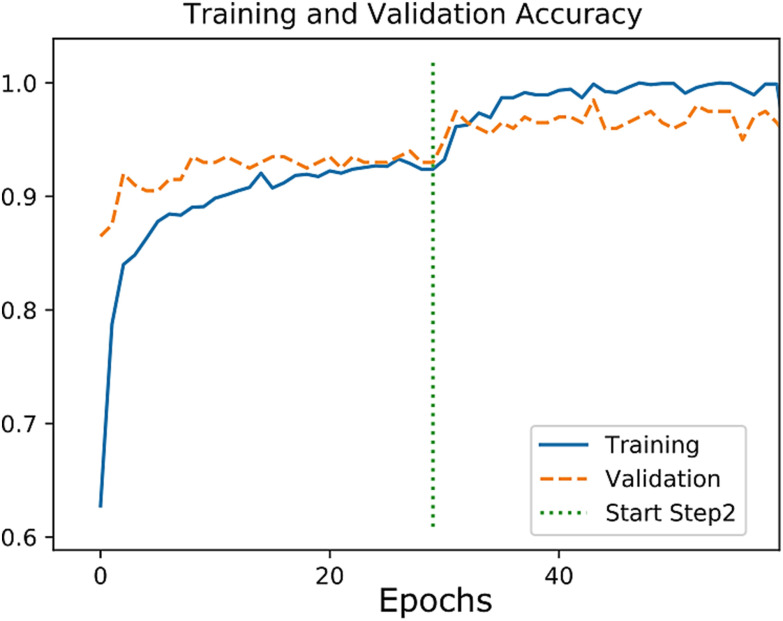
Fig. 4.

The Accuracy plot for the training of the NP phase.

All training sessions were performed using Adam [27] optimizer, the Categorical cross-entropy loss function, and the batch size of 5. All images were resized to the 224 × 224 pixels and preprocessed using the per-sample-standardization (i.e., zero mean and unit variance for each image intensities). Random rotation in the range of 0-15 degrees was used as the data augmentation on-the-fly (i.e., data augmentation is done at the training time).

In the NP phase, we perform our incremental domain adaptation method using the NP dataset. First, we freeze all layers of the base model except the last Conv block (Fig. 2(b)) and train the model for 30 epochs with the learning rate (LR) of 1e-4 as the warm-up step. Afterward, we unfreeze another Conv block (Fig. 2(c)) and continue the training for another 30 epochs but with a lower learning rate (LR = 1e-5). The last dense layer has two neurons in this phase.

In the CNP phase, we use the trained model of the previous phase and replace the last Dense layer with a new Dense layer with three neurons and retrain the model for another two steps. We freeze all layers of the base model (Fig. 2(a)) and train the classification layers (for 30 epochs with LR = 1e-4). Then, we unfreeze the last Conv block of the base (Fig. 2(b)) and continue the training (for 30 epochs with LR = 1e-5).

3). The CBMIR Model

The CBMIR algorithm characterizes an X-ray image by a convolutional neural network [4], [27]. The output of the corresponding encoder layer is then used as the feature vector, and it is encoded using a supervised kernel-based hashing function [28]. The hashing function converts high dimensional features into compressed binary codes, thus reducing the image recovery time and the memory required for hardware systems.

Feature extraction is a crucial step in a CBMIR system that can improve the results of retrieval. We employ CNN and integrate it with an autoencoder to extract image attributes. We train the autoencoder without supervision and keep the encoder part of the trained model for feature extraction. The CNN improves discrimination ability, and the autoencoder reduces the dimensionality of the extracted features [29].

The architecture of the encoder part of the CNN autoencoder is shown in Fig. 3. It accepts an X-ray image as its input and gives a 1 × 128 vector as its output. Based on our experience, the deep learning-based technique performs better than traditional methods, and it provides more efficient attributes when big data is available.

Fig. 3.

The architecture of the feature extraction network.

In recent years, hashing methods have been studied to represent big data. Concerning image retrieval, they are functions that accept an image or the corresponding feature vector and output a multi-bit number. Therefore, the search for similar data is performed in the binary field instead of a high-dimensional space. We employ a supervised hashing with kernels, which uses a limited number of labeled data to learn the similarity of two images. A kernel-based hashing function, defined in (1), is more appropriate for nonlinear data.

In (1), to are the samples from the training dataset, to are sets of coefficients, and b is the bias and is defined to normalize the whole training data (2).

In (2), n is the size of the training data. By substituting (2) in (1), we get (3).

where and is a vector map defined by , and . The kth hashing function () is defined in (4).

In (4), is the sign function, which gives 1/-1 for positive/negative inputs. Vector is obtained using labeled data. More details on the method are found in [28].

In the process of image retrieval, features are extracted from the query image by the CNN technique. The features are then converted to binary codes by the hashing method, and a search is performed among the available dataset.

4). The Visualization and Quantification Stage

In the case of an infected patient, we illustrate the lung volume, its vasculature structures, the GGOs, and the pulmonary lobes’ boundaries. Therefore, a physician observes disease progression and knows the number of lung lobes infected by the virus.

An essential measure for the severity of the illness is the CT Involvement Score that measures infection progress for individual lung lobes. Anatomically, the left lung is divided into Left Upper Lobe (LUL), Left Middle Lobe (LML), Left Lower Lobe (LLL). A right lung is split into Right Upper Lobe (RUL) and Right Lower Lobe (RLL). The proportional volume of the GGO in a lung lobe is rated from 0 to 5. Therefore, the total rate ranges from 0 to 25, corresponding to a healthy and fully infected lung, respectively. We calculate the CT score for each lobe and the whole lung as well.

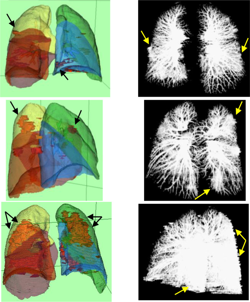
Visualization of the results consists of the Maximum Intensity Projection (MIP) of the lung, its vessels, and the GGOs in a 360˚ view. Moreover, we demonstrate the surface rendering of the lungs and the GGOs.

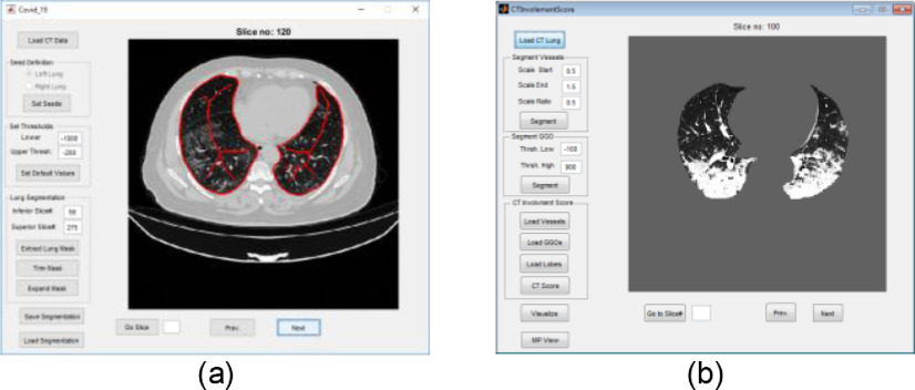
The first step of the quantification is the segmentation of the lung. We have developed a GUI in MATLAB environment to segment the lungs interactively. User-interaction is required since an infected lung has no homogenous texture, and most conventional lung segmentation algorithms fail in such cases. A user starts segmentation by brushing on a typical left and right lung slices as seeds. We call this slice the middle slice. The result of the thresholding of a middle slice is several disconnected objects. We label all objects that include a seed as the lung. The medial axis of the obtained mask is considered as seeds for the next images. Segmentation continues from the middle slice up to the superior and then to inferior directions. A trimming tool is implemented in the GUI as well. Then, we define the boundary of the lung lobes using the Slicer-CIP [30], [31]. The result of lobe segmentation fails when the GGO considerably infects the lung. In such cases, we use the lung's mask and the incomplete lobe masks of the Slicer-CIP and employ the Euclidean distance map to compensate for the lobes’ lost parts.

Concerning the segmentation of the GGOs, we follow a new approach. Since the intensity of the GGOs is similar to pulmonary vessels, we first delineate lung vasculatures by the Frangi method [32]. Then, we use the thresholding technique to find pixels in an approximate range of [−100, 900] and exclude extracted vessels from the previous step.

Visualization of the lung is performed in the C++ environment using the VTK toolkit. The mask of the lung is multiplied by the input CT image to extract the pulmonary tissue. Then, a snapshot of the MIP of the extracted lung is formed. The CT data is rotated axially by one degree, and a new MIP image is captured. All 360 MIP images are stored in an animated image format, and it is displayed to a physician. Moreover, the lung, its lobes, and GGOs are visualized by the surface rendering technique.

IV. Results

A. Classification Results

We evaluated the trained model of the NP phase on 200 test images. The loss and accuracy plots for the training and validation dataset are shown in Fig. 4. The Precision, Recall, F1-score, and confusion matrix results are shown in Table II and Table III, respectively. We achieved an accuracy of 0.97, a sensitivity of 0.99, and a specificity of 0.99 using the test set.

TABLE II. Results of the NP Phase on the NP Test Set.

Class	Precision	Recall	F1-score
Normal	0.98	0.97	0.97
Pneumonia	0.97	0.98	0.98

TABLE III. Confusion Matrix of the NP Phase on the NP Test Set.

	Normal	Pneumonia
Normal	97	3
Pneumonia	2	98

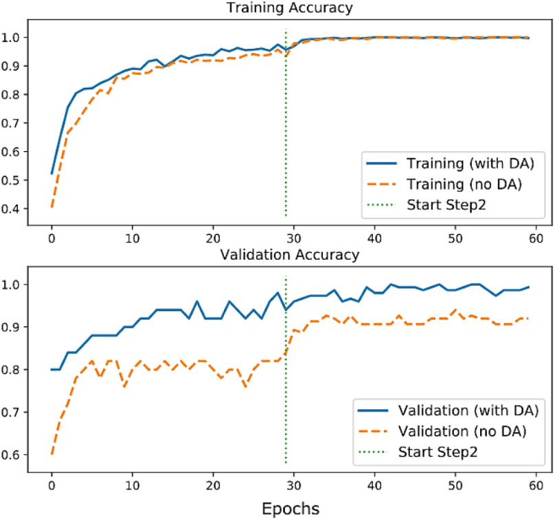
Concerning the CNP phase, we set up two experimental modes. In the first mode, we trained the model without the domain adaptation (i.e., without the NP phase). We call this mode as no_DA. In the second mode, we used the trained model from the NP phase and transferred its weight to the CNP model, then we improved training using the CNP dataset. We call this mode as with_DA.

Fig. 5 shows the comparison of the training accuracy between no_DA and with_DA modes. The generalization effect of the domain adaptation can be seen in the validation accuracy plot, where the performance of the CNP model with_DA is significantly better than the no_DA mode on the unseen test images.

Fig. 5.

Accuracy plots for two modes of the CNP phase.

The comparison of the accuracy and loss of the test images for the two modes of the CNP phase are listed in Table IV. Table V and Table VI show the predictions’ evaluation results on the test set for the CNP model (with_DA). The average prediction time was 0.26 seconds for each image.

TABLE IV. Results of the Two Modes of the CNP Phase on the CNP Test Set.

Class	Max. Accuracy	Min. Loss
CNP (no DA)	0.94	0.198
CNP (with DA)	0.97	0.032

TABLE V. Results of the CNP Phase (With DA) on the CNP Test Set.

Class	Precision	Recall	F1-score
COVID19	0.97	0.99	0.98
Normal	0.93	1.00	0.97
Pneumonia	1.00	0.91	0.95

TABLE VI. Results of the CNP Phase (With DA) on the CNP Test Set.

	COVID19	Normal	Pneumonia
COVID19	99	1	0
Normal	0	100	0
Pneumonia	3	6	91

The loss plots in Figs. 3 and 4 and the comparison of the results in Table IV showed that our incremental knowledge transfer and the domain adaptation had improved the baseline model (i.e., simple fine-tuning on the whole dataset). The promising results on the test set (provided in Table V and Table VI) also prove that the overfitting has not occurred on the training data.

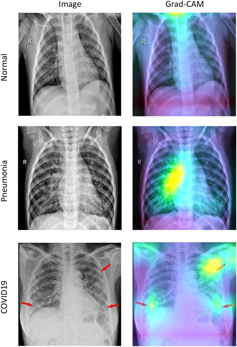
To visualize the model's attention on the input images, we used the Gradient-weighted Class Activation Mapping (Grad-CAM) method to visualize the model's attention on the input images [33]. With Grad-CAM, we can produce a heat map of the significant regions in the model's image. As depicted in Fig. 6, brighter zones are where the model activations are higher in the last convolutional layer for that specific image and its corresponding class label. We can see that the activations of the Normal case are almost identical for all regions. For the Pneumonia and COVID19 cases, some parts of the lungs are highlighted in the Grad-CAM's output. Our model uses these regions to decide on the class of the input image.

Fig. 6.

Sample X-ray images from each class and the output of the Grad-CAM for the corresponding category. Brighter regions are where the model activates more.

In Table VII, we compared our results with recent researches. As s shown in Table VII, we achieved the best sensitivity, specificity, and recall, among other methods. Moreover, the F-score, accuracy, and precision of our approach are comparable to other researches. Considering the number of coronavirus infected images that we used for testing, our algorithm achieved the best performance compared to state-of-the-art techniques.

TABLE VII. Comparison of the Results With Similar Methods.

Method	Dataset_Type (No. of test images)	F-Score (%)	Acc. (%)	Sen. (%)	Spec. (%)	Recall (%)	Prec. (%)
Zhang et al. [6]	COVID (50)–Pneumenia (717)	–	–	90.0	87.84	–	–
Narin et al. [3]	COVID (50), Healthy(50)	–	0.98	–	–	–	–
Mohammadi [14]	COVID(36)-Healthy(73)	99.0	99.1	–	–	98.0	100
Wang et al. [4]	COVID-19 (76), non-COVID-19 (8066)	–	92.4	80	–	–	–
Khan et al. [15]	COVID-19 (29), Healthy (72),Pneumenia (120)	95.6	95	–	97.5	96.9	95
Che Azemin [16]	COVID (154), Healthy(5828)	–	71.9	77.3	71.8	–	–
Jain et al. [17]	COVID-19(70), Healthy (85), Pneumenia (187)	–	97.77	–	–	97.14	97.14
Proposed method	COVID-19(100), Healthy (200), Pneumenia (200)	98	97	99	99	99	97

B. Retrieval Results

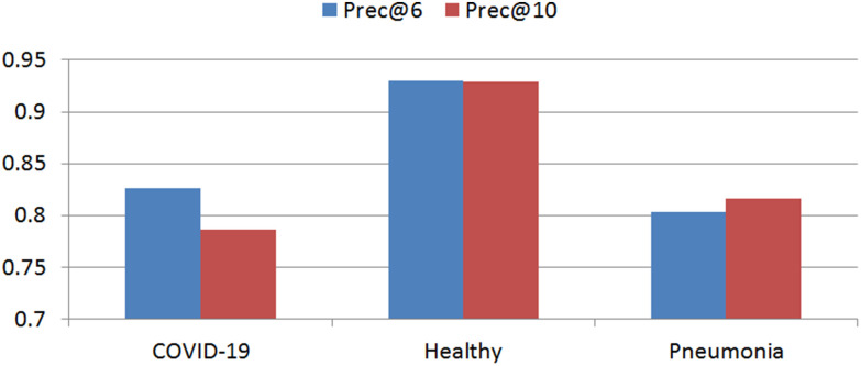
We used precision to quantify the retrieval performance of the proposed CBMIR framework. For a given query image, precision is the ratio of correctly retrieved instances. Its variations are Prec@6, Prec@10. Prec@k is the ratio of the accurately achieved images at top k-retrieved data. Results of precision for different image classes are shown in Fig. 7.

Fig. 7.

Retrieval results of the proposed CBMIR algorithm.

To verify the hashing method's effectiveness, we repeated retrieval of the test data without the hashing function. The total prec@6 of the COVID-19 result is reduced from 83% to 43%. In this case, most COVID-19 images are recognized as viral pneumonia.

Moreover, we used common test data to evaluate the CNN model and the CBMIR algorithm together. We utilized 22 -, 134 healthy, and 134 pneumonia X-ray images. The results show that the CNN model's accuracy (97%) is better than the CBMIR algorithm (89%). Concerning COVID-19, healthy, and pneumonia data, the two methods prepared similar results in 81%, 90%, and 71% of cases, respectively.

C. Visualization and Quantification Results

In Fig. 8(a) and (b), snapshots of the developed GUIs for segmentation of lung and quantification of the CTIS are shown. Moreover, in Fig. 9, MIPs and surface rendering of typical CT lungs are shown. In the first and second rows of Fig. 9, the CT scores are 5, and in the third row, the CTIS is 10. In Fig. 9, GGOs are shown as red objects in the surface rendering visualization. The GGOs are seen as white masses in the MIPs as well. Concerning Fig. 9, the CT scores of each lobe ([RUL, RML, RLL, LUL, LLL]) are [1, 1, 1, 1, 1], [1, 1, 1, 1, 1], and [1, 1, 3, 2, 3], corresponding to the first, second and third rows, respectively. The total lung volume scores are 5, 5, and 10, correspondingly to the first, second, and third rows.

Fig. 8.

Snapshots of the developed GUI for (a) segmentation of lung, and (b) quantification of the CTIS.

Fig. 9.

Surface rendering (Left column) and MIP (Right column) of three lung CT images. The CT scores of the first and second rows are 5, and that of the third row is 10. In the left column, GGOs are shown as red objects. Arrows emphasize the GGOs.

V. Discussion

Our solution to train the model accurately with a limited number of data is to use pre-trained models and domain adaptation strategy. As shown in Table VII, the proposed method outperforms methods like Wang et al. [4] and Che Azemin [16] using fewer images and no data augmentation. However, despite its remarkable performance, it seems that our model tends to make overconfident predictions. One reason can be the inter-class similarities in the NP dataset. The model, therefore, might have learned the preprocessing pattern of the NP dataset to predict the classes. This issue can be fixed by using appropriate preprocessing methods and randomized image alterations. Another solution is to include clinical knowledge in the training process. We believe that it is highly essential to use multi-domain techniques integrated with existing clinical experience.

Concerning the CBMIR model, we performed data separation linearly and retrieved the query images well using the hashing function. Moreover, we improved Prec@10 by 86.6% using the proposed deep features. Contrary to the CNN model, the results of the CBMIR is not influenced by the imbalanced class problem. Reducing the feature vectors’ size by the DNN reduces the memory cost and increases our algorithm's speed. Retrieval by the hashing function was performed in less than 0.03 seconds, which is less than the KNN (7.56 seconds) and KNN+PCA (0.07 seconds) [34]. To improve retrieval results, we need to utilize a more significant number of training data since hashing functions are more favored when big data is available.

Concerning visualization and quantification algorithms, the lung segmentation is a fundamental step for the next parts of the method. Delineation of the lung fails when the virus considerably infects it. In such cases, user interaction is a solution. Segmentation of the lobes has difficulties in the regions where there are GGOs and needs cooperation by a specialist. The slice thickness of the input data should be less than or equal to 1.5mm to obtain proper masks of lung and lobes. Therefore, we need to improve the available algorithms to include images with lower resolutions.

VI. Conclusion and Future Works

In this paper, we proposed a novel training method using incremental domain adaptation and knowledge transfer. We achieved state-of-the-art accuracy on the COVID-19 detection from the X-ray images. The proposed model was trained using a small set of available images, and it made high accuracy and generalization. The generalization can be improved with more training images. One future approach is to use an ensemble of different models or different imaging modalities like CT images to obtain more confidence in the results.

References

- [1].Corman V. M. et al. , “Detection of 2019 novel coronavirus (2019-nCoV) by real-time RT-PCR,” Eurosurveillance, vol. 25, no. 3, 2020, Art. no. 2000045. [DOI] [PMC free article] [PubMed] [Google Scholar]
- [2].Wang S. et al. , “A deep learning algorithm using CT images to screen for corona virus disease (COVID-19),” Eur. Radio., Feb. 2020, pp. 1–9. [DOI] [PMC free article] [PubMed]
- [3].Narin A., Kaya C., and Pamuk Z., “Automatic detection of coronavirus disease (COVID-19) using X-ray images and deep convolutional neural networks,” 2020, arXiv: 2003.10849. [DOI] [PMC free article] [PubMed]
- [4].Wang L., Lin Z.Q., and Wong A., “COVID-Net: A tailored deep convolutional neural network design for detection of COVID-19 cases from chest X-ray images,” Sci. Rep., vol. 10, no. 1, pp. 1–12. [DOI] [PMC free article] [PubMed] [Google Scholar]
- [5].Ghoshal B. and Tucker A., “Estimating uncertainty and interpretability in deep learning for coronavirus (COVID-19) detection,” arXiv:2003.10769.
- [6].Zhang J., Yutong X.Yi L., Chunhua S., and Yong X., “COVID-19 screening on chest X-ray images using deep learning based anomaly detection,” 2020, arXiv:2003.12338.
- [7].Accessed: Apr. 2, 2021. [Online]. Available: https://radiologyassistant.nl/chest/covid-19/covid19-imaging-findings#chest-ct-ground-glass
- [8].Imaging Technology News: Accessed: Apr. 2, 2021, [Online]. Available: https://www.itnonline.com/content/ct-provides-best-diagnosis-novel-coronavirus-covid-19
- [9].Xie X., Zhong Z., Zhao W., Zheng C., Wang F., and Liu J., “Chest CT for typical 2019-nCoV pneumonia: Relationship to negative RT-PCR testing,” Radiology, 2020, Art. no. 200343. [DOI] [PMC free article] [PubMed]
- [10].Zhao W., Zhong Z., Xie X., Yu Q., and Liu J., “Relation between chest CT findings and clinical conditions of coronavirus disease (COVID-19) pneumonia: A multicenter study,” Amer. J. Roentgenol., vol. 214, no. 5, pp. 1072–1077, 2020. [DOI] [PubMed] [Google Scholar]
- [11].Chung M. et al. , “CT imaging features of 2019 novel coronavirus (2019-NCoV),” Radiology, vol. 295, no. 1, pp. 202–207, 2020. [DOI] [PMC free article] [PubMed] [Google Scholar]
- [12].Pan F. et al. , “Time course of lung changes at chest CT during recovery from coronavirus disease 2019 (COVID-19),” Radiology, vol. 295, no. 3, pp. 715–721, Jun. 2020. [DOI] [PMC free article] [PubMed] [Google Scholar]
- [13].Ng M.-Y. et al. , “Imaging profile of the COVID-19 infection: Radiologic findings and literature review,” Radiol. Cardiothorac. Imag., vol. 2, no. 1, Feb. 2020, p. e200034. [DOI] [PMC free article] [PubMed] [Google Scholar]
- [14].Mohammadi R., Salehi M., Ghaffari H., Rohani A. A., and Reiazi R., “Transfer learning-based automatic detection of coronavirus disease 2019 (COVID-19) from chest X-ray images,” J. Biomed. Phys. Eng., vol. 10, no. 5, pp. 559–568, 2020. [DOI] [PMC free article] [PubMed] [Google Scholar]
- [15].Khan A. I., Shah J. L., and Bhat M. M., “CoroNet: A deep neural network for detection and diagnosis of COVID-19 from chest X-ray images,” Comput. Methods Programs Biomed., 2020, Art. no. 105581. [DOI] [PMC free article] [PubMed]
- [16].Che Azemin M. Z., Hassan R., Mohd Tamrin M. I., and Md Ali M. A., “COVID-19 deep learning prediction model using publicly available radiologist-adjudicated chest X-ray images as training data: Preliminary findings,” Int. J. Biomed. Imag., vol. 2020, Art no. 8828855. [DOI] [PMC free article] [PubMed]
- [17].Jain G., Mittal D., Thakur D., and Mittal M. K., “A deep learning approach to detect covid-19 coronavirus with X-ray images,” Biocybern. Biomed. Eng., vol. 40, no. 4, pp. 1391–1405, 2020. [DOI] [PMC free article] [PubMed] [Google Scholar]
- [18].Kermany D. S., Zhang K., and Goldbaum M., “Labeled optical coherence tomography (oct) and chest X-ray images for classification,” Mendeley data, vol. 2, no. 2, Jun. 2018. [Google Scholar]
- [19].Cohen J. P., Morrison P., and Dao L., “COVID-19 image data collection,” 2020, arXiv:2003.11597.
- [20].Abadi M. et al. , “TensorFlow: Large-scale machine learning on heterogeneous distributed systems,” 2016, arXiv:1603.04467.
- [21].The Visualization Toolkit: Accessed: June 5, 2020. [Online]. Available: https://vtk.org/
- [22].Simonyan K. and Zisserman A., “Very deep convolutional networks for large-scale image recognition,” 2015, arXiv:1409.1556.
- [23].Deng J., Dong W., Socher R., Li L.-J., Li K., and Fei-Fei L., “ImageNet: A large-scale hierarchical image database,” in Proc. IEEE Conf. Comput. Vis. Pattern Recognit., 2009, pp. 248–255. [Google Scholar]
- [24].Szegedy C., Vanhoucke V., Ioffe S., Shlens J., and Wojna Z., “Rethinking the inception architecture for computer vision,” in Proc. IEEE Comput. Soc. Conf. Comput. Vis. Pattern Recognit., 2016, vol. 2016-Dec., pp. 2818–2826. [Google Scholar]
- [25].Huang G., Liu Z., Van Der Maaten L., and Weinberger K. Q., “Densely connected convolutional networks,” in Proc. 30th IEEE Conf. Comput. Vis. Pattern Recognit., 2017, pp. 2261–2269. [Google Scholar]
- [26].Kingma D. P. and Ba J. L., “Adam: A method for stochastic optimization,” in Proc. 3rd Int. Conf. Learn. Representations Conf. Track Proc., 2015. [Google Scholar]
- [27].Springenberg J. T., Dosovitskiy A., Brox T., and Riedmiller M., “Striving for simplicity: The all convolutional net,” 2014, arXiv:1412.6806. [Google Scholar]
- [28].Liu W., Wang J., Ji R., Jiang Y. G., and Chang S. F., “Supervised hashing with kernels,” in Proc. IEEE Comput. Soc. Conf. Comput. Vis. Pattern Recognit., 2012, pp. 2074–2081. [Google Scholar]
- [29].Yu J., Zheng X., and Wang S., “A deep autoencoder feature learning method for process pattern recognition,” J. Process Control, vol. 79, pp. 1–15, 2019. [Google Scholar]
- [30].Estépar R. S. J., Ross J. C., Harmouche R., Onieva J., Diaz A. A., and Washko G. R., “C66 LUNG IMAGING II: NEW PROBES AND EMERGING TECHNOLOGIES: Chest Imaging Platform: An Open-Source Library And Workstation For Quantitative Chest Imaging,” Amer. J. Respir. Critical Care Med., vol. 191, no. 1, 2015. [Google Scholar]
- [31].Onieva J. et al. , “Chest imaging platform: An open-source library and workstation for quantitative chest imaging,” Int. J. Comput. Assist. Radiol. Surg., vol. 11, no. 1, pp. S40–S41, 2016. [Google Scholar]
- [32].Frangi A. F., Niessen W. J., Vincken K. L., and Viergever M. A., “Multiscale vessel enhancement filtering,” in Proc. Int. Conf. Med. Image Comput. Comput.-Assist. Intervention, 1998, pp. 130–137. [Google Scholar]
- [33].Selvaraju R. R., Cogswell M., Das A., Vedantam R., Parikh D., and Batra D., “Grad-CAM: Visual explanations from deep networks via gradient-based localization,” in Proc. IEEE Int. Conf. Comput. Vis., 2017, vol. 2017-October, pp. 618–626. [Google Scholar]
- [34].Zhang X., Liu W., and Zhang S., “Mining histopathological images via hashing-based scalable image retrieval,” in Proc. IEEE 11th Int. Symp. Biomed. Imag., 2014, pp. 1111–1114. [Google Scholar]