Classification of Severe and Critical Covid-19 Using Deep Learning and Radiomics

Abstract

Objective: The coronavirus disease 2019 (COVID-19) is rapidly spreading inside China and internationally. We aimed to construct a model integrating information from radiomics and deep learning (DL) features to discriminate critical cases from severe cases of COVID-19 using computed tomography (CT) images. Methods: We retrospectively enrolled 217 patients from three centers in China, including 82 patients with severe disease and 135 with critical disease. Patients were randomly divided into a training cohort (n = 174) and a test cohort (n = 43). We extracted 102 3-dimensional radiomic features from automatically segmented lung volume and selected the significant features. We also developed a 3-dimensional DL network based on center-cropped slices. Using multivariable logistic regression, we then created a merged model based on significant radiomic features and DL scores. We employed the area under the receiver operating characteristic curve (AUC) to evaluate the model's performance. We then conducted cross validation, stratified analysis, survival analysis, and decision curve analysis to evaluate the robustness of our method. Results: The merged model can distinguish critical patients with AUCs of 0.909 (95% confidence interval [CI]: 0.859–0.952) and 0.861 (95% CI: 0.753–0.968) in the training and test cohorts, respectively. Stratified analysis indicated that our model was not affected by sex, age, or chronic disease. Moreover, the results of the merged model showed a strong correlation with patient outcomes. Significance: A model combining radiomic and DL features of the lung could help distinguish critical cases from severe cases of COVID-19.

I. Introduction

In December 2019, a novel coronavirus broke out and rapidly spread globally [1]. On 12 February, 2020, the World Health Organization (WHO) announced the official name of the pneumonia caused by this virus: coronavirus disease 2019 (COVID-19) [2]. COVID-19 manifests as acute respiratory distress syndrome and is highly infectious [3]. On September 1, 2020, more than 84,000 patients in China, and more than 27 million globally had a confirmed case of COVID-19 [4]. Thus, healthcare systems have been severely burdened by this emergent virus. Patients with COVID-19 are classified into mild, moderate, severe, and critical ill subgroups according to disease severity, which is estimated using chest imaging and clinical performance [5]. Initially, the research [6] reported that among 72314 cases from Chinese, approximately 14% are severe patients and 5% are critical patients. However, the incidence of comorbidities was significantly higher in the critical group than in the severe group among 476 patients recruited from three hospitals in Wuhan, Shanghai, and Anhui cities [7]. Importantly, patients with a critical case of COVID-19 have a higher mortality rate than severe and moderate COVID-19 patients among 710 COVID-19 cases in Wuhan city and 90 cases in Chongqing city [8], [9]. Therefore, early diagnosis and improved treatment of critical COVID-19 patients are key to reducing mortality.

Radiomics can improve the diagnostic and prognostic performance of medical systems via high-throughput mining of quantitative features from medical images [10], [11]. Deep learning (DL) has also been successfully applied in disease screening and diagnosis [12], [13]. Several researchers have suggested that radiomics and DL may be valuable in screening COVID-19 [14], [15]. Computed tomography (CT) is a great supplement to real-time reverse-transcription polymerase chain reaction (RT-PCR) testing in the diagnosis and assessment of COVID-19 severity. Some typical features found on chest CT in severe COVID-19 cases are ground-glass opacities (GGOs), consolidation, and bilateral patchy shadowing in the lung [16], [17]. However, the CT characteristics are somewhat similar between severe and critical cases [9]. Especially, most severe, and critical patients showed involvement of multiple lung lobes in the CT scans. Furthermore, patients from severe and critical groups presented with similar higher MuLBSTA (multilobular infiltrates, lymphocyte, bacterial coinfection, smoking, hypertension, and age) scores than the moderate group [7]. In addition, severe and critical patients are associated with the same clinical symptoms, including fever, dry cough, shortness of breath, and so on [17]. Therefore, it is crucial to extract high–throughput information to identify disease severity. To our knowledge, no studies have differentiated critical cases from severe cases based on medical imaging.

In this study, we seek to combine different level information between both machine learning and deep learning algorithms to identify COVID-19 disease severity grade based on CT images. This paper makes the following major contributions. Firstly, we implemented an automatic segmentation algorithm to segment the lung region for hand-crafted feature extraction and deep learning model construction. Secondly, we determined the optimal hand-crafted feature subset from 102 features for classifying severe and critical cases. We implemented a variety of feature selection algorithms to filter significant features. Thirdly, we constructed one 3D convolutional network which could capture high-level semantic information and further identify the disease severity. Finally, we utilized four machine learning algorithms to combine hand-crafted and deep learning features and obtained higher precision. Extensive experiments were implemented and results demonstrated the superiority of our proposed methods.

The remainder of this paper is organized as follows. In Section II, we introduce the theory of methods. In Section III, we present the results of the experiments. Finally, we conclude in Section V.

II. Materials and Methods

A. Patients

Our institutional review board approved this retrospective study, waiving the requirement for informed consent. A total of 217 patients diagnosed with severe or critical COVID-19 from three centers were enrolled in the study (Renmin Hospital of Wuhan University [number of patients [n] = 199 from a total of 321 patients with COVID-19], Henan Provincial People's Hospital [n = 9 from a total of 64 patients], and First Affiliated Hospital of Anhui Medical University [n = 9 from a total of 61 patients]). All patients were diagnosed between 6 January and 26 February, 2020, and all were confirmed to have COVID-19 via nucleic acid testing. The inclusion criteria were as follows: (1) availability of transverse non-contrast enhanced chest CT images, (2) severe or critical COVID-19, and (3) less than 1 week between CT scan and COVID-19 diagnosis. The CT acquisition protocols were detailed in Supplementary 1.

The diagnosis of severe and critical illness was based on the Diagnosis and Treatment of Novel Coronavirus Pneumonia of China [5]. Patients who met any of the following criteria were diagnosed as critically ill: respiratory failure requiring mechanical ventilation, shock, organ failure requiring intensive care.

After the CT examination, 137 patients were followed up for at least 12 days. The endpoints were poor outcomes, including death, mechanical ventilation, or ICU admission before 26 March, 2020.

We randomly selected 80% of the patients as a training cohort and the rest as a test cohort. Fig. 1 depicts the flowchart of our study, which included automated CT image segmentation, radiomic feature extraction, feature selection, DL network construction, merged model construction, and model analysis.

Fig. 1.

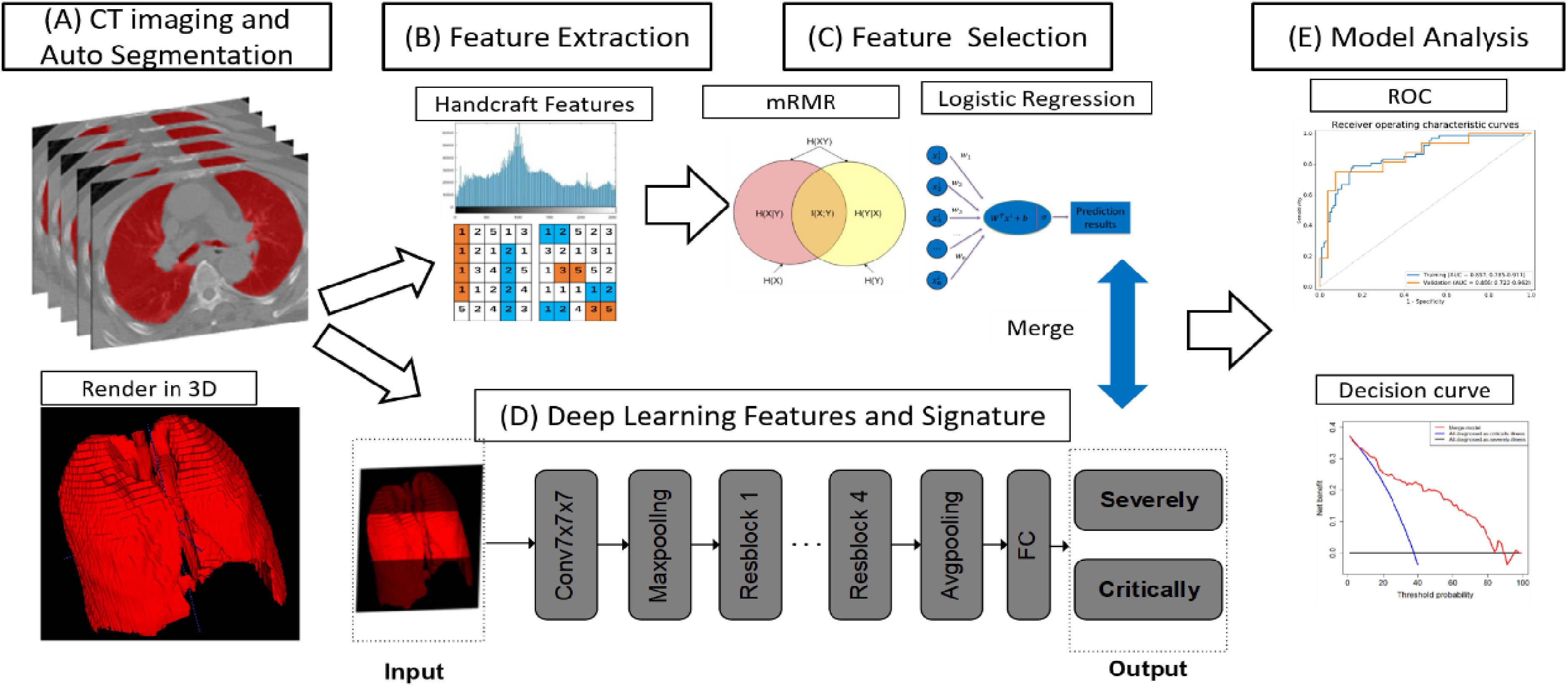
The pipeline of merged model construction. CT, computed tomography. For each CT image, we obtained 3D ROI (A), from which the radiomic features were extracted (B). After feature selection, we obtained the optimal feature set (C). Meanwhile, deep learning model was constructed (D). The performance of merged model which integrating radiomics and deep learning features was evaluated (E).

B. Automated CT Image Segmentation

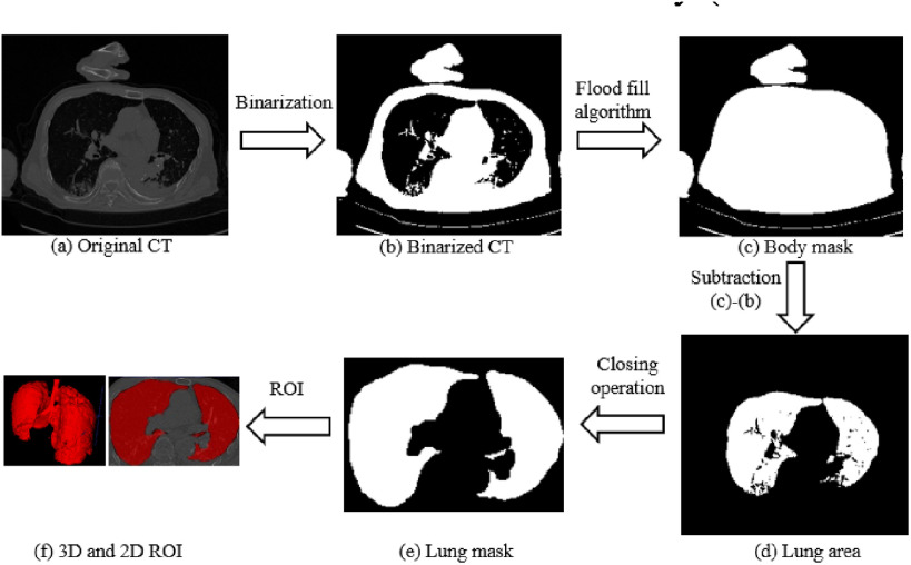
In the implementation phase, we developed an automated segmentation algorithm to extract whole lung volume [18]. The preliminary lung region was first isolated by applying a threshold of value for air in the human body (Hounsfield Units = -300) to binary CT images. Next, given the initial seed nodes [coordinates = (0,0,0)] in the preliminary non-body region, a flood-fill algorithm detected nodes that were connected to the initial seeds in three dimensions and generated the connected domains of the body. Note that, flood fill algorithm determines the area connected to a given node in a multi-dimensional array. After that, we subtracted the binarized CT from the body connectivity map to obtain the lung area. Then a closing operation, the basic workhorse of morphological noise removal, was applied to remove small holes. Finally, we selected slices that contained connected domains of the lung. The automated segmentation process is depicted in Fig. 2. All CT images were then resized to 40 × 243 × 243. Next, we utilized lung volume corresponding binary volume masks to extract radiomic features, then center-cropped the lung volume to a size of 20 × 243 × 243 to focus on the central slice of lung volume [19]. The cropped lung volume was then inputted into our 3D DL model.

Fig. 2.

Flow chart of the automatic segmentation algorithm (axial view).

C. Radiomic Feature Extraction and Selection

To reduce the impact of differences in equipment and scanning parameters, we resampled CT images into 1 × 1 × 5 mm voxel spacing using tri-linear interpolation [20]. We then extracted 102 radiomic features from the 3-dimensional (3D) lung volume, comprising three types: (1) shape features (number of features [m] = 14), which quantified the size and shape of the lung volume, (2) first-order features (m = 18), which described the distribution of voxel intensities within the lung volume, and (3) texture features (m = 70), which quantified the relationships between neighboring voxels. Feature extraction was implemented using Python language (https://www.python.org) and based on Pyradiomics [21].

Feature selection was conducted to select the optimal feature subset [22]. Specifically, the Mann–Whitney U test was applied to evaluate the correlation between features and severity grade (severe or critical), as well as to screen out the significant features (P < 0.05). Next, the minimum redundancy maximum relevancy (mRMR) algorithm was used to rank features according to their relevance to severity grade and their redundancy with other features. The top-ranked 20 features remained. Finally, the most representative features were selected using a backward stepwise approach, according to the Akaike information criterion (AIC) [23]. The details of key algorithms as follows:

1). Minimum-Redundancy Maximum-Relevancy (mRMR)

The purpose of mRMR algorithm is to find an optimal feature set with features based on mutual information which is defined as:

where , are two given random variables, , , are their probability density functions.

The algorithm contains two parts: “Maximum-Relevancy” to find features that having a maximum dependency on prediction label. “Minimum-Redundancy” to eliminate redundant features and result in a more compact feature set without any sensible performance degradation. Suppose we have selected m-1 features from feature set . The feature will be selected from by maximization of the following criterion:

where is the prediction label, and are different features.

2). Backward Stepwise

We implemented backward stepwise to select features according to the Akaike information criterion. AIC is a standard to measure the goodness of model fitting and tends to prefer a most fitted model with the simplest parameters. Backward stepwise algorithm starts with all the variables in the model, and at each step, a variable may be removed according to AIC, finally the model with the minimal AIC can be found. AIC was defined as follows:

where is the number of model parameters and is the likelihood function.

In this way, we screened out the optimal feature set for further analysis. Meanwhile, we compared differences in the distribution of discriminative features between severe and critical cases using a violin plot.

D. Deep-Learning Network Construction

Considering the relatively small amount of data and the huge amount of 3D convolution model parameters, in order to prevent overfitting and facilitate training, we built a DL network based on 3D-Resnet-10 [24], [25]. The detailed structure is shown in Fig. 3. The center-cropped lung volume was fed into this network, which was stacked with a 7 × 7 × 7 convolution layer, a max-pooling layer, and four residual blocks. Convolution layers utilize various kernels to convolve feature maps to capture the high-level semantic information. Pooling layers were used to reduce the dimensions of feature maps. Each residual block contained two 3 × 3 × 3 convolution layers and a shortcut connection. The residual blocks make the network easy to optimize. Importantly, all the convolution layers were followed by a batch normalization layer which enables faster and more stable training of the network. After a global average pooling layer, we obtained a 512-length, 1-dimensional vector that reflected the phenotype of lung volume. Finally, the vector was fed into the fully connected layer and the non-linear activation layer to predict illness severity.

Fig. 3.

The structure of the 3D deep learning network.

We implemented the DL network using Pytorch (version = 1.1.0) framework and Python 3.6 (https://www.python.org/). We randomly selected one-fifth of training cohort samples as a validation set for hyperparameter optimization. Afterward, the learning rate and weight decay were set to 1e-5 and 1, respectively. For alleviating the issue of the class balance, we adopted a weighted random sampler method in each batch. All the parameters were initialized randomly and trained from scratch. The Adam optimizer, together with binary cross-entropy loss, was applied to update the parameters of 3D-Resnet-10. We trained the network on the training cohort for 60 epochs. All the operations of the deep learning model were implemented on a workstation equipped with 64 Intel (R) Xeon (R) Gold 6130 CPU @ 2.10GHz and one GPU of Titan RTX Graphics Card with 12GB of memory.

E. Merged Model Construction and Analysis

Four machine learning classifiers, including logistic regression, support vector machine (SVM), decision tree, and random forest, were constructed based on the optimal radiomic features subset and the results obtained from the DL network for comparison. Note that, all the variables were normalized with z-score normalization in the training and test cohorts using the corresponding mean and standard deviation. All the hyper-parameters are tuned using 10-fold cross-validation and the GridSearchCV function in the Scikit-learn library on the training cohort. The discrimination performance of the classifier was evaluated by 100 iterations 10-fold cross-validation on the entire dataset. Meanwhile, we calculated the relative standard deviation (RSD) to quantify the stability of different classifiers. RSD is defined as follows:

where and were the standard deviation and mean of the AUC values respectively. It should be mentioned that higher stability of classifiers corresponds to lower RSD.

All the classifiers were constructed based on open-sourced scikit learn package using python language. Furthermore, the best-performing classifier logistic regression was termed as the merged model which combines the information of radiomics and DL. Note that, we removed insignificant features during the process of model construction. Thus, we got the final merged model that could predict the illness severity of patients. For further comparison, we constructed four machine learning classifiers solely based on the optimal radiomic feature subset, and the best-performing classifier logistic regression was termed the Rad model. In addition, the 3D DL network was termed the DL model, with the results called the DL-score. For logistic regression, based on linear regression, the formula is as follows:

where is the results of logistic regression representing the probability, is the coefficient corresponding to feature , is the number of features, and is the intercept of linear regression.

The area under the receiver operating characteristic (ROC) curve (AUC), the area under the precision-recall curve (PR-AUC), accuracy, sensitivity, and specificity were calculated to quantify the prediction performance of our model. Accuracy, sensitivity, and specificity were calculated in terms of the threshold determined by maximizing Youden index of the training cohort. Accuracy, sensitivity, specificity, and Youden index were defined as follows:

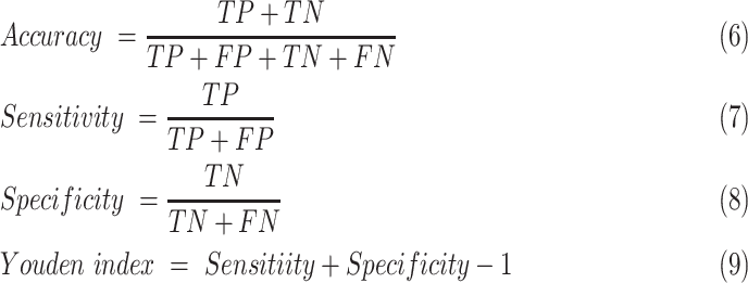where TP is the number of true positive samples, TN is the true negative samples, FP is the false positive samples and FN is the false negative samples.

To evaluate the robustness of our model, we performed a stratified analysis that took into account age, sex, and chronic disease. Meanwhile, the predictive abilities of different ROCs were compared using the Delong test. A violin plot was used to compare the distribution of severe and critical cases according to the predictions of the model. The net reclassification index (NRI) was used to compare performance between the Rad model, DL model, and merged model, as well as to quantify the improvement in predictive performance [26]. Decision curve analysis (DCA) was performed to estimate the clinical utility of our model. Finally, we investigated the prognostic value of the merged model in patients who had follow-up information. It should be mentioned that the optimal cutoff point was determined by X-tile software (version 3.6.1; Yale University School of Medicine, New Haven, CT, USA) [27].

F. Cross Validation

In order to evaluate the robustness of the proposed method, we performed 5-fold cross-validation on the entire dataset. Specifically, the whole dataset was randomly split into five-folds, with four folds used for model training, while the remaining one for testing. The above training-testing procedures were repeated five times with a mean AUC computed accordingly.

G. Statistical Analysis

The Mann–Whitney U test and chi-squared test were used to assess the correlations between clinical factors and illness severity. Two-sided P-values < 0.05 indicated statistical significance. The 95% confidence interval [CI] was estimated by 1000-time bootstrap in the training and test cohorts. Statistical analysis was conducted using R software (version 3.3.4; http://www.Rproject.org).

III. Results

A. Patient Characteristics

Patients were divided into a training cohort (86 males, 88 females; average age, 61.22 ± 15.86 years) and a test cohort (26 males, 17 females; average age, 56.67 ± 16.49 years). Table I describes the clinical characteristics of the training and test cohorts. The univariate analysis showed that age and chronic disease had significant correlations with illness severity (P < 0.05), indicating that old patients with chronic disease (such as diabetes, hypertension, and other diseases) tend to be diagnosed with a critical illness. In contrast, we found that sex, manufacturer, and slice sickness were not associated with illness severity.

TABLE I. Clinical Characteristics of Patients.

	Training cohort (174)			Test cohort (43)
	Severe (108)	Critical (66)	P-Value	Severe (27)	Critical (16)	P-Value
Age	56.56±14.70	68.85±14.80	< 0.001*	51.81±14.23	64.88±17.21	0.024*
Sex			0.906			0.663
Male	53 (49%)	33 (50%)		17 (63%)	9 (56%)
Female	55 (51%)	33 (50%)		10 (37%)	7 (44%)
Chronic disease			0.003*			0.228
With chronic disease	29 (27%)	32 (48%)		7 (26%)	7 (44%)
Without chronic disease	79 (73%)	34 (52%)		20 (74%)	9 (56%)
			0.519			0.522
GE CT scanner	101 (94%)	64 (97%)		25 (93%)	16 (100%)
Other CT scanner	7 (6%)	2 (3%)		2 (7%)	0 (0%)
Slice Thickness			0.086			0.283
> 1 mm	10 (9%)	1 (2%)		4 (15%)	0 (0%)
≤ 1 mm	98 (91%)	65 (98%)		13 (85%)	16 (100%)

B. Selection and Validation of Radiomic Features

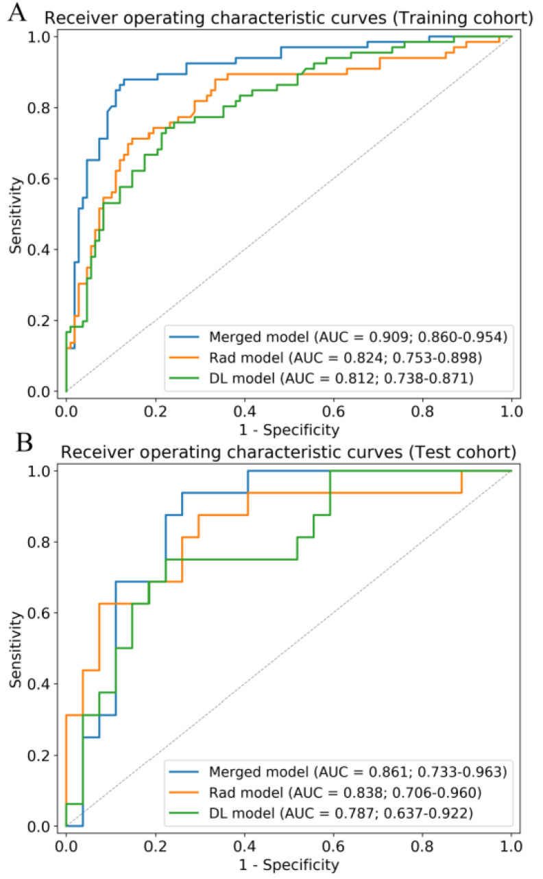
During feature extraction, 66 significant features were screened out after the Mann–Whitney U test. The top 20 features were then selected according to the mRMR algorithm. Finally, six features were selected after backward stepwise selection. The physical details of the features are shown in Supplementary 2. The detailed performance of four machine learning classifiers is shown in Supplementary 3. Results showed that the performance of models based on handcrafted features is inferior to those of models based on both deep learning and handcrafted features. The formula of the Rad model was as follows: 5.819 × firstorder_RootMeanSquared + 1.932 × glcm_ClusterShade - 1.888 × firstorder_10Percentile - 4.607 × glcm_DifferenceVariance - 3.418 × glcm_Correlation - 1.404 × gldm_SmallDependenceHighGrayLevelEmphasis - 0.657. More details are shown in Table II. The Rad model exhibited good performance for discriminating critical illness in the training cohort (AUC: 0.824, [CI]: 0.742–0.892) and test cohort (AUC: 0.838, 95% CI: 0.688–0.958). Fig. 4 shows the ROC curves of the Rad model in the training and test cohorts.

TABLE II. Risk Factors of the Rad and Merged Model.

Variable	Rad model			Merged model
	β	Adjusted OR (95% CI)	P-value	β	Adjusted OR (95% CI)	P-value
Intercept	-0.657		< 0.001*	-0.778		< 0.001*
firstorder_10Percentile	-1.888	0.151 (0.057–0.354)	< 0.001*	-1.491	0.459 (0.284–0.715)	< 0.001*
firstorder_RootMeanSquared	5.819	3.4e+2 (48.948–3.2e+3)	< 0.001*
glcm_ClusterShade	1.932	6.901 (2.538–22.726)	< 0.001*
glcm_DifferenceVariance	-4.607	0.010 (0.001–0.066)	< 0.001*	-1.009	0.364 (0.155–0.806)	0.015*
glcm_Correlation	-3.418	0.033 (0.006–0.137)	< 0.001*	-0.946	0.388 (0.198–0.715)	0.003*
gldm_SmallDependenceHighGrayLevelEmphasis	-1.404	0.246 (0.079–0.554)	0.004*	-1.198	0.302 (0.117–0.623)	0.005*
DL-score				3.684	39.810 (14.597 –134.978)	< 0.001*

Fig. 4.

Receiver operating characteristic curves of the merged model, Rad model, and DL model in the training (A) and test (B) cohorts. AUC, area under the receiver operating characteristic curve.

C. Deep Learning Model and Merged Model Construction

We trained a 3D-Resnet-10 network based on lung volume to generate the DL model. The whole training process takes roughly one hour and the inference for each CT data takes about one second. ROC curves of the DL model are shown in Fig. 4, demonstrating that DL can distinguish critical cases from severe cases. The yield AUCs of the DL model were 0.812 (CI: 0.743–0.874) and 0.787 (CI: 0.627–0.929) in the training and test cohorts, respectively.

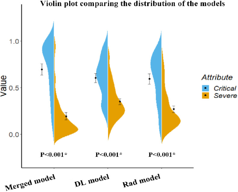
To combine the information from the radiomic features (Rad model) with that from the high-level features (DL model), we constructed four machine learning classifiers based on the optimal radiomic features set and the DL score. Hyper-parameters of classifiers and average performance of 100 times 10-fold cross-validation are depicted in Table III. According to the table, SVM has the lowest performance among the four classifiers. Although the decision tree and random forest show higher performance on the training cohort, the performance on the test cohort is low, which indicates that classifiers are overfitting to a certain extent. Interestingly, logistic regression shows good performance on both the training and test cohort and has the lowest RSD which demonstrates the stability of this classifier. Afterward, we utilized logistic regression to construct our merged model. We also removed the insignificant features in this process. Finally, we obtained the merged model and the corresponding formula was as follows: 3.684 × DL-score – 0.946 × glcm_Correlation – 1.198 × gldm_SmallDependenceHighGrayLevelEmphasis – 1.491 × firstorder_10Percentile – 1.009 × glcm_DifferenceVariance – 3.684.More details are shown in Table II. The merged model showed encouraging performance in the training cohort (AUC: 0.909, 95% CI: 0.859–0.952) and test cohort (AUC: 0.861, 95% CI: 0.753–0.968). More detailed performance parameters are listed in Table IV. The corresponding ROC curves are shown in blue lines in Fig. 4. In the test cohort, the merged model had significant better performance than the Rad model (Delong test: P = 0.009; NRI: 0.156, P = 0.008) and DL model (Delong test: P < 0.001; NRI: 0.184, P = 0.002). Additionally, the violin plot revealed significant differences in the distribution of the models’ prediction between severe and critical cases, as shown in Fig. 5.

TABLE III. Performance and Hyper-Parameters of Four Classifiers Based on Handcrafted Features and DL Score.

Classifiers	Hyper-parameters	RSD (%)	Training AUC (mean±SD)	Test AUC (mean±SD)
Logistics Regression	C = 1000 Penalty = ‘L1’	8.092	0.854±0.010	0.848±0.097
SVM	C = 0.125 Gamma = ‘10.0’ Kernel = ‘rbf’	8.203	0.806±0.010	0.804±0.093
Decision Tree	Criterion = ‘gini’ Min samples leaf = 19 Min samples split = 2	9.541	0.900±0.011	0.805±0.092
Random Forest	Criterion = ‘gini’ Min samples leaf = 5 Min samples split = 2 Max features = ‘auto’ N estimators = 10	10.20	0.981±0.004	0.839±0.085

TABLE IV. Performance Evaluation of Models.

Index(95% CI)	Training Cohort					Test Cohort
	Rad model	DL model		Merged model		Rad model		DL model		Merged model
Thre	0.458		0.426		0.346		0.458		0.426		0.346
Acc	0.799 (0.733-0.855)		0.764 (0.709-0.824)		0.874 (0.809-0.909)		0.744 (0.670-0.825)		0.767 (0.685-0.850)		0.814 (0.710-0.875)
Sen	0.712 (0.606-0.823)		0.742 (0.661-0.848)		0.879 (0.787-0.952)		0.750 (0.653-0.882)		0.750 (0.650-0.870)		0.875 (0.750-1.000)
Spe	0.852 (0.773-0.917)		0.778 (0.704-0.854)		0.870 (0.791-0.922)		0.741 (0.639-0.852)		0.778 (0.687-0.880)		0.778 (0.655-0.852)
PR-AUC	0.761 (0.647-0.849)		0.738 (0.650-0.841)		0.854 (0.750-0.932)		0.718 (0.615-0.807)		0.694 (0.560-0.848)		0.798 (0.675-0.907)
AUC	0.824 (0.753–0.898)		0.812 (0.738–0.871)		0.909 (0.860–0.954)		0.838 (0.706–0.960)		0.787 (0.637–0.922)		0.861 (0.733–0.963)

Fig. 5.

Violin plot comparing the distribution of the models’ prediction of severe and critical COVID-19 cases. This plot also includes an error bar. The distributions of the features were compared using the Mann–Whitney U test.

D. Cross Validation

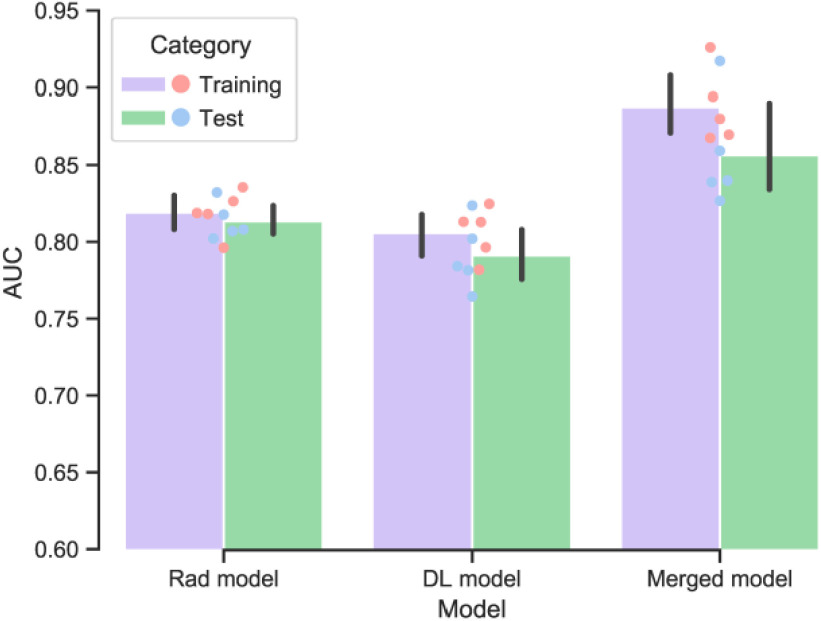
In the 5-fold cross-validation experiments, the mean AUC of the merged model was found to be 0.855 (range: 0.827–0.917) and RSD = 3.81 in the test cohort, indicating satisfactory method robustness. Meanwhile, the Rad model and DL model also show stable performance. The performance of the merged model is significantly better than the other models (P < 0.05). A bar plot of the cross-validation result is shown in Fig. 6 and detailed performance of each fold is shown in Supplementary 4.

Fig. 6.

Performance of the developed models in the training and test cohorts using five-fold cross-validation. For each iteration, 80% of patients were used as the training cohort and the remaining patients as the test cohort.

E. Stratified Analysis

As shown in Fig. 7, we performed three stratified analyses on all patients: age, sex, and chronic diseases. In terms of age stratification, we set the cutoff as the median age of all patients (61 years). Chronic diseases included diabetes, hypertension, and chronic pulmonary disease. The results showed that the merged model worked well, regardless of the situation, and that it was not affected by age (P = 0.95 by Delong test), sex (P = 0.63 by Delong test), or chronic diseases (P = 0.13 by Delong test). In addition, the accuracy of our merged model in the subgroup with slice thicknesses greater than 1mm is 0.933 and in the subgroup with slice thickness less than 1 mm is 0.856.

Fig. 7.

Stratified analysis of merged model based on (A) age, (B) sex, and (C) chronic disease. AUC, area under the receiver operating characteristic curve.

F. Decision Curve Analysis

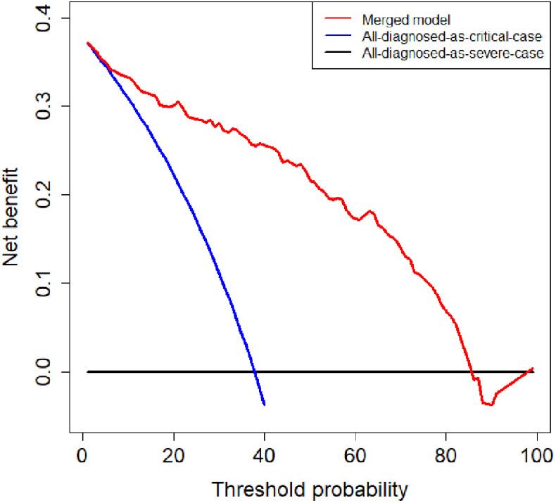
To evaluate the clinical utility of the merged model, we conducted a decision curve analysis. As shown in Fig. 8, if the threshold probability of the clinical decision was between 7% and 85%, then using the merged model to predict the severity of patients adds more benefit than treating either all or no patients as critical cases.

Fig. 8.

Decision curve analysis of the merged model. The red, blue, and black lines represent the merged model, the hypothesis that all patients diagnosed as critical cases, and the hypothesis that all patients diagnosed as severe cases, respectively. The y-axis represents the net benefit. The x-axis represents the threshold probability. The threshold probability is where the expected benefit of further treatment is equal to the expected benefit of avoiding further treatment. For example, if the possibility that patient is critical case over the threshold probability, then further treatment for a critical cases should be adopted.

G. Follow-Up Analysis

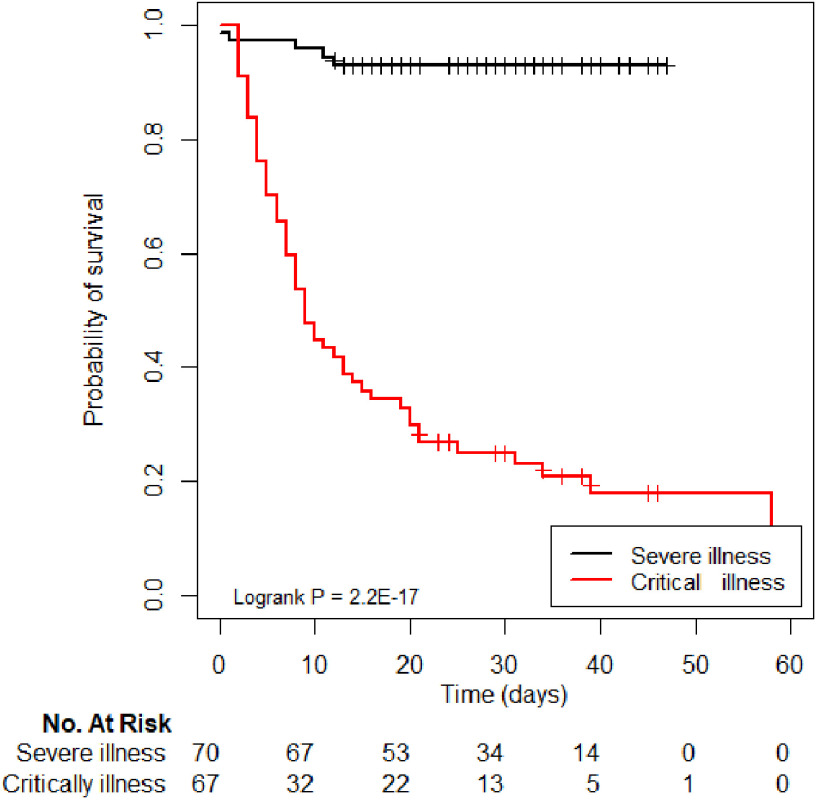
Furthermore, we successfully followed up with 137 patients. The Kaplan–Meier survival curve based on merged model is depicted in Fig. 9, stratified by severity grade, and compared using two-sided log-rank tests. In addition, the Kaplan–Meier survival curves of Rad and DL models are shown in Supplementary 5. Results show that merged model has better stratification performance than Rad and DL models. Notably, we found that the outcome of the merged model was significantly different between the severe and critical illness severities (P < 0.001).

Fig. 9.

Kaplan–Meier curves of severe and critical cases, based on the predictions of the merged model.

IV. Discussion

In the present study, based on a multi-center dataset, we constructed a merged model that integrates radiomic and DL features to distinguish critical from severe COVID-19 cases. The study found that both DL score and handcrafted features can be independent predictors of a severity grade. The merged model showed encouraging discriminative ability to screen out critical cases, as well as a strong correlation with the prognosis of patients. Furthermore, the stratified analysis demonstrated the robustness of our model, indicating that our study findings may play an important role in the detection of critical COVID-19 cases.

COVID-19 causes critical illness, and poor outcomes have drawn social attention. Several studies have focused on the clinical characteristics and imaging features of critical cases. For example, Li et al. [9] pointed out that severe and critical cases have similar features on CT images, namely consolidation, linear opacities, bronchial wall thickening, lymph node enlargement, pericardial effusion, and pleural effusion that are more pronounced than in moderate cases. Based on CT imaging and clinical features, those authors constructed a model to screen out severe and critical patients from mild and moderate patients; the model showed good performance. Patients with critical COVID-19 have a high mortality rate, which should be studied more in future investigations [8], [28]. However, it is difficult for radiologists to distinguish critical cases from severe cases based on chest CT alone. In the present study, the proposed merged model could discriminate critical cases from severe cases. As such, the model could be used to provide supplemental information for medical staff during treatment. In addition, the results of the merged model show a strong correlation with the outcome, as the critical cohort showed a high probability of a poor outcome.

The present study utilized an automated algorithm to segment the whole lung volume and extract radiomic features. We set a CT Hounsfield Unit value of -300 as a threshold for lung volume segmentation. Therefore, the 3D region of interest (ROI) could represent the whole information of the lung volume and may have been less influenced by manual delineation. As such, the robustness and repeatability of the model may have been improved than models based on manual delineation. In addition, the DL model was built on slices that contained the ROI and center cropped in three dimensions before being fed into the DL network. In this way, most other organs and tissues were blocked, irrelevant noise information was eliminated from the picture, and the convergence of the network was accelerated.

Radiomic features can be used to quantify the lung volume. After feature selection, six significant features were obtained. Among the selected features, firstorder_RootMeanSquared, firstorder_10Percentile, and glcm_ClusterShade depicted the distribution of the voxel intensity, while glcm_Correlation, glcm_DifferenceVariance, and gldm_SmallDependenceHighGrayLevelEmphasis depicted the correlation between neighboring voxels. For instance, firstorder_10Percentile indicated the 10^th percentile of intensity in the 3D-ROI. To our knowledge, the area of the CT lesion increases with disease severity. Therefore, firstorder_10Percentile was intrinsically related to the severity of illness. Furthermore, these features might contain texture information about lung volume, allowing the Rad model to distinguish critical cases.

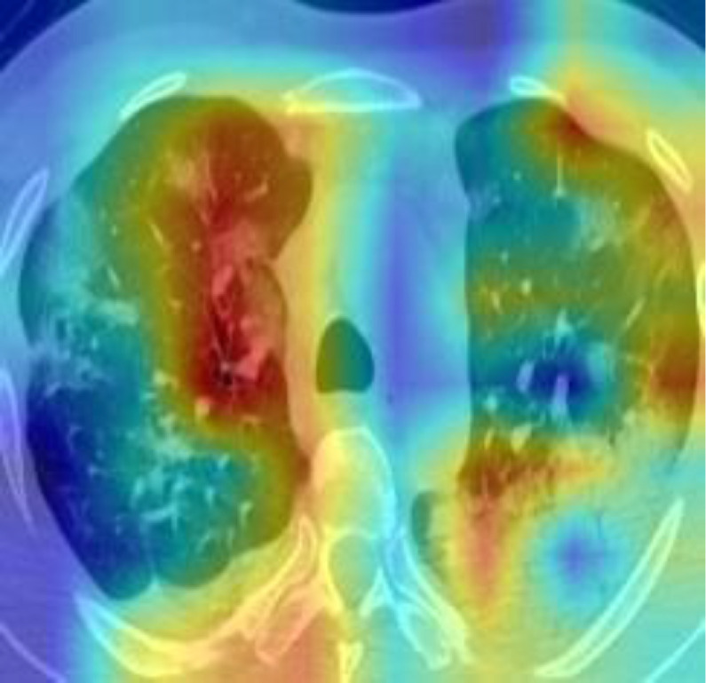
DL model was conducted to extract the high-level of the lung areas for making the final decision. In order to demonstrate the good interpretability of our DL model, we exploited Gradient Weighted Activation Mapping (Grad-CAM) to visualize the region which plays an important role during the inference [29]. Fig. 10 shows one slice of the CT images from the test cohort, and with the Grad-CAM overlaid on it. It reveals our DL model is able to detect the suspected lesions and make the corresponding diagnosis.

Fig. 10.

Visualization map of one slice of the CT images from the test cohort and corresponding Grad-CAM.

Several studies have demonstrated complementarity between handcraft features and DL features [30]–[33]. In the present study, we integrated the information from radiomic and DL features using multivariable logistic regression. Consequently, the merged model utilized low-level and high-level information to achieve better performance in both the training and test cohorts. Results of the 5-fold cross-validation experiment on the entire dataset also demonstrate the feasibility of the proposed method.

The stratified analysis demonstrated the robustness of the merged model. We performed three stratified analyses, taking into account sex, age, and chronic diseases. The results showed that our model was not affected by these factors. Interestingly, we found that our merged model has better performance on the CT images with a slice thickness greater than 1mm. Maybe because our dataset is relatively small, and the influence of slice thickness on our merged model needs further research. Some studies have pointed out that older age and chronic diseases such as hypertension and diabetes should be considered as risk factors for poor prognosis of COVID-19 [34], [35]. Notably, age and chronic disease differed significantly between the severe and critical cases in our training cohort. However, the performance of the merged model showed no significant difference between the younger group (AUC = 0.884) and the elderly group (AUC = 0.887) or between patients with chronic diseases (AUC = 0.896) and those without chronic diseases (AUC = 0.896). Interestingly, the results of the merged model showed a strong correlation with poor COVID-19 outcome.

The clinical application of our merged model contains the following steps. 1) Exclude the mild and moderate COVID-19 patients based on clinical manifestations. 2) Collect CT images. 3) Segment lung area using an automatic segmentation algorithm. 4) Extract significant hand-crafted features and calculate DL-score by utilizing the trained 3D-ResNet-10 network. 5) Merge hand-crafted features and DL-score. Finally, we obtained the possibility that the patient is a critical case. All the steps take about half a minute for one patient. In our study, patients with outcome of merged model greater than 0.346 were termed as potential critical cases. Consequently, additional treatment such as respiratory support, convalescent plasma treatment, immunotherapy and so on could be adopted to reduce the mortality.

The present study had several limitations. Firstly, the sample size of the dataset was relatively small. A larger, multi-centered dataset is necessary for further studies. Secondly, more complete clinical information needs to be collected; clinical characteristics also have predictive ability, which could be used to further improve the performance of the merged model. Finally, the 3D-Resnet-10 network that we used was not pretrained. Pretraining the model on a large public dataset might improve the performance of our model.

V. Conclusion

In conclusion, we constructed a merged model integrating the information of radiomic features and DL features. The model could distinguish critical cases of COVID-19 from severe cases. The results of the model showed a strong correlation with patient outcomes. The key of our proposed method is to combine two types of features to get a better model, so it is also suitable for other different classification tasks.

Funding Statement

This work was supported by the National Key R&D Program of China under Grants 2017YFC1308700, 2017YFA0205200, 2017YFC1309100, and 2016YFC0102600 in part by the National Natural Science Foundation of China under Grants 82022036, 91959130, 81971776, 81771924, 6202790004, 81930053, 61622117, and 81671759, in part by the Scientific Instrument Developing Project of the Chinese Academy of Sciences under Grant YZ201672, in part by the Beijing Natural Science Foundation under Grants L182061, JQ19027 in part by the Strategic Priority Research Program of Chinese Academy of Sciences under Grant XDB 38040200, in part by the Beijing Nova Program under Grant Z181100006218046, in part by the Project of High-Level Talents Team Introduction in Zhuhai City under Grant Zhuhai HLHPTP201703, and in part by the Youth Innovation Promotion Association CAS under Grant 2017175.

References

- [1].Huang C. et al. , “Clinical features of patients infected with 2019 novel coronavirus in Wuhan, China,” Lancet, vol. 395, no. 10223, pp. 497–506, 2020. [DOI] [PMC free article] [PubMed] [Google Scholar]
- [2].“World Health Organization. World experts and funders set priorities for COVID-19 research,” [Online]. Available: https://www.who.int/news-room/detail/12-02-2020-world-experts-and-funders-set-priorities-for-covid-19-research
- [3].Paules C. I., Marston H. D., and Fauci A. S., “Coronavirus infections—More than just the common cold,” JAMA, vol. 323, no. 8, pp. 707–708, 2020. [DOI] [PubMed] [Google Scholar]
- [4].“COVID-19 CORONAVIRUS PANDEMIC,” [Online]. Available: https://www.worldometers.info/coronavirus/?utm_campaign = CSauthorbio?
- [5].“National health commission of the people's republic of China. Diagnosis and treatment protocols of pneumonia caused by a novel coronavirus (trial version 5),” [Online]. Available: http://www.nhc.gov.cn/yzygj/s7653p/202002/3b09b894ac9b4204a79db5b8912d4440.shtml
- [6].Wu Z. and McGoogan J. M., “Characteristics of and important lessons from the coronavirus disease 2019 (COVID-19) outbreak in China: Summary of a report of 72 314 cases from the chinese center for disease control and prevention,” JAMA, vol. 323, no. 13, pp. 1239–1242, 2020. [DOI] [PubMed] [Google Scholar]
- [7].Feng Y. et al. , “COVID-19 with different severities: A multicenter study of clinical features,” Amer. J. Respir. Crit. Care Med., vol. 201, no. 11, pp. 1380–1388, 2020. [DOI] [PMC free article] [PubMed] [Google Scholar]
- [8].Yang X. et al. , “Clinical course and outcomes of critically ill patients with SARS-CoV-2 pneumonia in Wuhan, China: A single-centered, retrospective, observational study,” Lancet Respir. Med., vol. 8, no. 5, pp. 475–481, 2020. [DOI] [PMC free article] [PubMed] [Google Scholar]
- [9].Li K. et al. , “The clinical and chest CT features associated with severe and critical COVID-19 pneumonia,” Invest. Radiol., vol. 55, no. 6, pp. 327–331, 2020. [DOI] [PMC free article] [PubMed] [Google Scholar]
- [10].Dong D. et al. , “Development and validation of an individualized nomogram to identify occult peritoneal metastasis in patients with advanced gastric cancer,” Ann. Oncol., vol. 30, no. 3, pp. 431–438, 2019. [DOI] [PMC free article] [PubMed] [Google Scholar]
- [11].Lambin P. et al. , “Radiomics: Extracting more information from medical images using advanced feature analysis,” Eur. J. Cancer, vol. 48, no. 4, pp. 441–446, 2012. [DOI] [PMC free article] [PubMed] [Google Scholar]
- [12].Bi W. L. et al. , “Artificial intelligence in cancer imaging: Clinical challenges and applications,” CA. Cancer J. Clin., vol. 69, no. 2, pp. 127–157, 2019. [DOI] [PMC free article] [PubMed] [Google Scholar]
- [13].Yue H. et al. , “Machine learning-based CT radiomics model for predicting hospital stay in patients with pneumonia associated with SARS-CoV-2 infection: A multicenter study,” Ann. Transl. Med., vol. 8, no. 14, p. 859, 2020. [DOI] [PMC free article] [PubMed] [Google Scholar]
- [14].Zhavoronkov A. et al. , “Potential COVID-2019 3C-like protease inhibitors designed using generative deep learning approaches,” Insilico Med. Hong Kong Ltd A, vol. 307, 2020, Art. no. E1. [Google Scholar]
- [15].Li L. et al. , “Artificial intelligence distinguishes COVID-19 from community acquired pneumonia on chest CT,” Radiology, 2020, Art. no. 200905.
- [16].Bernheim A. et al. , “Chest CT findings in coronavirus disease-19 (COVID-19): Relationship to duration of infection,” Radiology, 2020, Art. no. 200463. [DOI] [PMC free article] [PubMed]
- [17].Zhang J. et al. , “Clinical characteristics of 140 patients infected with SARS-CoV-2 in Wuhan, China,” Allergy, vol. 75, no. 7, pp. 1730–1741, 2020. [DOI] [PubMed] [Google Scholar]
- [18].Januszewski M. et al. , “High-precision automated reconstruction of neurons with flood-filling networks,” Nat. Methods, vol. 15, no. 8, pp. 605–610, 2018. [DOI] [PubMed] [Google Scholar]
- [19].Meng L. et al. , “2D and 3D CT radiomic features performance comparison in characterization of gastric cancer: A multi-center study,” IEEE J. Biomed. Heal. Inf., 2020. doi: 10.1109/JBHI.2020.3002805. [DOI] [PubMed]
- [20].Gumaei A., Hassan M. M., Hassan M. R., Alelaiwi A., and Fortino G., “A hybrid feature extraction method with regularized extreme learning machine for brain tumor classification,” IEEE Access, vol. 7, pp. 36266–36273, 2019. [Google Scholar]
- [21].Van Griethuysen J. J. M. et al. , “Computational radiomics system to decode the radiographic phenotype,” Cancer Res, vol. 77, no. 21, pp. e104–e107, 2017. [DOI] [PMC free article] [PubMed] [Google Scholar]
- [22].Sohail A. S. M., Bhattacharya P., Mudur S. P., and Krishnamurthy S., “Selection of optimal texture descriptors for retrieving ultrasound medical images,” in Proc. IEEE Int. Symp. Biomed. Imag.: From Nano Macro, 2011, pp. 10–16. [Google Scholar]
- [23].Sakamoto Y., Ishiguro M., and Kitagawa G., “Akaike information criterion statistics,” Dordrecht, Netherlands D. Reidel, vol. 81, 1986. [Google Scholar]
- [24].He K., Zhang X., Ren S., and Sun J., “Deep residual learning for image recognition,” in Proc. IEEE Conf. Comput. Vis. Pattern Recognit., 2016, pp. 770–778. [Google Scholar]
- [25].Yang C., Rangarajan A., and Ranka S., “Visual explanations from deep 3D convolutional neural networks for alzheimer's disease classification,” in Proc. AMIA Annu. Symp. Proc., 2018, vol. 2018, Art. no. 1571. [PMC free article] [PubMed] [Google Scholar]
- [26].Pencina M. J., D'Agostino R. B. Sr., D'Agostino R. B. Jr, and Vasan R. S., “Evaluating the added predictive ability of a new marker: From area under the ROC curve to reclassification and beyond,” Statist. Med., vol. 27, no. 2, pp. 157–172, 2008. [DOI] [PubMed] [Google Scholar]
- [27].Camp R. L., Dolled-Filhart M., and Rimm D. L., “X-tile: A new bio-informatics tool for biomarker assessment and outcome-based cut-point optimization,” Clin. cancer Res., vol. 10, no. 21, pp. 7252–7259, 2004. [DOI] [PubMed] [Google Scholar]
- [28].Murthy S., Gomersall C. D., and Fowler R. A., “Care for critically ill patients with COVID-19,” JAMA, vol. 323, no. 15, pp. 1499–1500, 2020. [DOI] [PubMed] [Google Scholar]
- [29].Selvaraju R. R., Cogswell M., Das A., Vedantam R., Parikh D., and Batra D., “Grad-cam: Visual explanations from deep networks via gradient-based localization,” in Proc. IEEE Int. Conf. Comput. Vis., 2017, pp. 618–626. [Google Scholar]
- [30].Forghani R., Savadjiev P., Chatterjee A., Muthukrishnan N., Reinhold C., and Forghani B., “Radiomics and artificial intelligence for biomarker and prediction model development in oncology,” Comput. Struct. Biotechnol. J., vol. 17, 2019, Art. no. 995. [DOI] [PMC free article] [PubMed] [Google Scholar]
- [31].Dong D. et al. , “Deep learning radiomic nomogram can predict the number of lymph node metastasis in locally advanced gastric cancer: An international multi-center study,” Ann. Oncol., vol. 31, no. 7, pp. 912–920, 2020. [DOI] [PubMed] [Google Scholar]
- [32].Wu J. M.-T. et al. , “Applying an ensemble convolutional neural network with savitzky–golay filter to construct a phonocardiogram prediction model,” Appl. Soft Comput., vol. 78, pp. 29–40, 2019. [Google Scholar]
- [33].Hassan M. M., Alam M. G. R., Uddin M. Z., Huda S., Almogren A., and Fortino G., “Human emotion recognition using deep belief network architecture,” Inf. Fusion, vol. 51, pp. 10–18, 2019. [Google Scholar]
- [34].Guo W. et al. , “Diabetes is a risk factor for the progression and prognosis of COVID-19,” Diabetes. Metab. Res. Rev., vol. 36, no. 7, 2020, Art. no. e3319. [DOI] [PMC free article] [PubMed] [Google Scholar]
- [35].Zhou F. et al. , “Clinical course and risk factors for mortality of adult inpatients with COVID-19 in Wuhan, China: A retrospective cohort study,” Lancet, vol. 395, no. 10229, pp. 1054–1062, 2020. [DOI] [PMC free article] [PubMed] [Google Scholar]