CycFlowDec: A Python module for decomposing flow networks using simple cycles

Abstract

New algorithms for determining the expected flow through simple cycles in a closed network are presented. Current network analysis software do not implement algorithms for expected cyclic flow decomposition, despite its potential value. Decomposing networks into expected cycle flows provides a quantitative characterization of network cycles that can be further analyzed for sensitivity and correlative behavior. An efficient, general algorithm has been coded into CycFlowDec, an open source Python module available at https://github.com/austenb28/CycFlowDec.

Code metadata

Current code version	v1
Permanent link to code/repository used for this code version	https://github.com/ElsevierSoftwareX/SOFTX-D-20-00084
Code Ocean compute capsule	N/A
Legal Code License	GPL 3.0
Code versioning system used	Git
Software code languages, tools, and services used	Python 3
Compilation requirements, operating environments & dependencies	Python 3, NumPy
If available Link to developer documentation/manual	https:/github.com/austenb28/CycFlowDec
Support email for questions	a.bernardi@utah.edu

1. Motivation and significance

Network analysis is a practice that reaches all areas of science, from biology [1], to computer science [2], to traffic flow [3]. For some analyses, a central objective is to characterize the expected flow of certain cycles within a network [1,4,5]. However, quantifying the relative probabilities of pathways through a complex network is generally non-trivial. Many graph theoretic algorithms have been developed to characterize network flow [6–9], and the software implementing these algorithms have gained popularity [10–15]. These methods generally quantify the maximum flow or minimum cost paths. However, there has been limited progress on the determination of the expected flow decomposition of complex networks. Previous studies concerning expected cycle flows have been largely theoretical [16,17], and have focused on developing mathematical descriptions of related system attributes, such as entropy production rates [18], or specific network types, such as quantum Markov semigroups [19].

The primary motivator of this work involves the analysis of relevant ion transport pathways in a kinetic Markov state model of a Cl⁻/H⁺ antiporter, [1,20,21] for which decomposing the network into expected simple cyclic flows is essential. These cycles can be further studied to determine their sensitivities to specific transitions, revealing sub-ensemble properties and opening new avenues for mechanistic insight. Aside from this specific application, the Python module CycFlowDec, described in this work, has been designed to decompose a given flow network into expected simple cycle flows. Any chemical reaction network can be analyzed using CycFlowDec to quantitatively determine the expected flow of relevant reaction cycles. This feature is particularly valuable for analyzing networks in the fields of catalysis, such as the study of enzymatic networks or heterogeneous catalysis. Precise knowledge of expected cycle flows in reactive networks provides a quantitative metric for the importance of the underlying mechanisms that dictate the functionality of the reactive network. In an analogous fashion, CycFlowDec can be applied to the analysis of any application involving flow networks. For example, one could use CycFlowDec to determine the expected cycle flows in a communications network [22], a traffic network [23], a migration network [24], or a monetary network [25].

2. Theoretical background

New algorithms for decomposing a closed flow network into simple cycles are presented herein. Note that a simple cycle is a cycle that contains at most one instance of any node. Thus, an expected simple cycle flow decomposition assigns the expected flows to all simple cycles in a network such that the original flow network is recovered when the cycle flows are summed together. The mathematical framework of the algorithms presented in this work is based on the work developed in Ref. [26] and expanded on in chapter 3 of Ref. [27]. This section presents an overview of this previously developed framework, while the appendices describe the newly developed algorithms. The most efficient, general algorithm has been implemented in the CycFlowDec Python module, available at https://github.com/austenb28/CycFlowDec with examples and additional documentation. While the presented algorithms are designed to decompose closed flow networks into simple cycle flows, the framework can be straightforwardly extended to open networks via transformation of the open network to an effective closed network. This is accomplished by including an additional virtual node, which connects the network sinks to the sources.

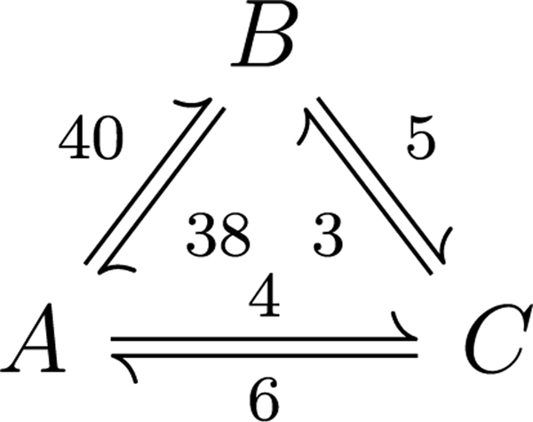
Four algorithms are sequentially outlined in Appendix A, ending with the fastest algorithm, which is incorporated in CycFlowDec. We begin with a brief overview of the underlying theory [26,27]. Consider the three-node flow network ${\mathbb{\text{N}}}^3$ in Fig. 1. Let a representative cyclic walk W on ${\mathbb{\text{N}}}^3$ be

$$W=\{A,B,A,C,B,A,B,C,B,C,A\}.$$

Walk W can be decomposed into simple cycles with the following procedure: [27]

1. Start at the first node of W. Mark it as visited.

2. Walk to the next node.

3. If the current node was already marked as visited, extract all nodes from its previous visitation up to the preceding node. Log the cycle composed by the extracted nodes. Mark the extracted nodes as unvisited except the current node. Otherwise, mark the current node as visited.

4. Repeat 2 and 3 until the end of the walk.

Fig. 1.

The three-node flow network ${\mathbb{\text{N}}}^3$.

Note that a simple cycle is a cycle that contains no more than one instance of any node. Table 1 illustrates the decomposition of W using the described procedure. A cycle that cycles through q nodes n₁, n₂, . . ., n_q, . . . is denoted by (n₁, n₂, . . ., n_q). Extracting cycles with this procedure has several benefits. If the procedure is performed on a network $\mathbb{\text{N}}$ using a random walk generated via Markovian transition probabilities, we can define the divergent limit [27]

$$\underset{N\to \infty }{\lim }{w}_c^N=w_c\forall c\in ℂ,$$ (1)

where N is the length of the walk, C is the set of all simple cycles on $\mathbb{\text{N}}$, and $w_c^N$ is the number of extracted cycles c on a walk of length N. Eq. (1) represents the primary basis of all algorithms described in this work. The expected probability p_c of a cycle is given by [27]

$$p_c=w_c{\left(\sum _{\forall j\in ℂ}{w}_j\right)}^{-1}\forall c\in ℂ.$$ (2)

Table 1.

Walk-based simple cycle extraction example. The current node on W is in bold.

W	Visited	Extracted cycle
{A, B, A, C, B, A, B, C, B, C, A}	{A}
{A, B, A, C, B, A, B, C, B, C, A}	{A, B}
{A, C, B, A, B, C, B, C, A}	{A}	(A, B)
{A, C, B, A, B, C, B, C, A}	{A, C}
{A, C, B, A, B, C, B, C, A}	{A, C, B}
{A, B, C, B, C, A}	{A}	(A, C, B)
{A, B, C, B, C, A}	{A, B}
{A, B, C, B, C, A}	{A, B, C}
{A, B, C, A}	{A, B}	(B, C)
{A, B, C, A}	{A, B, C}
{A}	{A}	(A, B, C)

Importantly, p_c is finite and takes on the same value irrespective of the starting node of the walk. The expected flow of a cycle c, given as f_c, may be calculated as

$$f_c=w_c{\left(\sum _{\forall k\in ℂ}{n}_k{w}_k\right)}^{-1}\sum _{\forall j\in \mathbb{E}}{e}_j\forall c\in ℂ,$$ (3)

where $\mathbb{\text{E}}$ is the set of all edges on $\mathbb{\text{N}}$, e_j is the flow of edge j, and n_k is the number of edges in cycle k. Combining Eqs. (2) and (3) shows that f_c is also finite and takes on the same value irrespective of the starting node of the walk. Eq. (3) is the equation used in CycFlowDec to calculate cycle flows.

3. Software description

CycFlowDec is an open source Python module that enables the expected simple cycle flow decomposition of closed networks. Flow decomposition is accomplished using the percolating with burn-in and minimum contribution tolerance described in Appendix A.4, enabling rapid and efficient performance on complex networks.

3.1. Software architecture

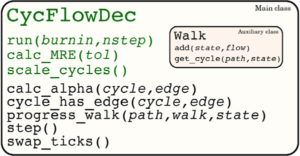
CycFlowDec is fully contained in a single, compact Python 3 script, requiring NumPy as its only external library. The object oriented structure uses a CycFlowDec main class, employing various methods for decomposition and analysis. An auxiliary Walk class is also used that enables efficient tracking of the percolating walks in the algorithm. A diagram of the architecture of CycFlowDec is provided in Fig. 2. Detailed descriptions of the classes and methods along with examples are available at https://github.com/austenb28/CycFlowDec.

Fig. 2.

CycFlowDec architecture diagram. Classes and methods intended for general users are in green.

4. Illustrative examples

4.1. Algorithm performances

In order to assess the performance of the cyclic flow decomposition algorithms described in Appendix A, the mean relative error (MRE) was calculated between edges of the reconstructed flow network from cycles and the original flow network. That is,

$$\text{MRE}=\frac{1}{N_E}\sum _{j\in \mathbb{E}}\frac{1}{e_j}\left|e_j-\sum _{k\in {ℂ}_j}{f}_k\right|,$$ (4)

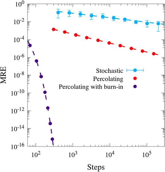
where N_E is the number of edges in $\mathbb{\text{N}}$, and $\mathbb{\text{C}}$_j is the set of simple cycles containing edge j. Fig. 3 shows the MRE vs. steps for the first three described algorithms for ${\mathbb{\text{N}}}^3$, the three-node network specified in Fig. 1. The percolating with burn-in uses burn = N − 2, where N is the total number of steps. Optimizing the selection of burn is discussed in Appendix B. The ${\mathbb{\text{N}}}^3$ network is small enough to use a minimum contribution tolerance of zero. The percolating with burn-in algorithm is significantly faster than the stochastic and percolating algorithms, exhibiting geometric instead of algebraic convergence. CycFlowDec employs the percolating with burn-in and minimum contribution tolerance algorithm, permitting rapid cyclic flow decomposition of closed networks.

Fig. 3.

Log–log plot of MRE vs. algorithm steps for the stochastic, percolating, and percolating with burn-in algorithms for ${\mathbb{\text{N}}}^3$. Stochastic and percolating have trendlines of the form y = ax^−b, and percolating with burn-in uses y = ae^−bx.

The ${\mathbb{\text{N}}}^3$ cyclic flow decomposition for the previously described algorithms is reported in Table 2. All three algorithms appear to be converging to the same decomposition, consistent with the fact that they are based on the same fundamental theory. Consistent with the final datapoints in Fig. 3, the stochastically determined cycle flows agree with the higher accuracy algorithms by at least one digit, while the percolating cycle flows agree with the percolating with burn-in by at least four digits.

Table 2.

Cycle flows of ${\mathbb{\text{N}}}^3$ by algorithm. N = 2 × 10⁵ for stochastic and percolating, while N = 300 for percolating with burn-in.

Cycle	Stochastic	Percolating	Percolating, burn = N − 2
(A, B)	36.90029	36.77424	36.77419
(A, C)	2.74282	2.77420	2.77419
(B, C)	1.78229	1.77418	1.77419
(A, B, C)	3.18206	3.22579	3.22581
(A, C, B)	1.20101	1.22580	1.22581

4.2. Additional networks

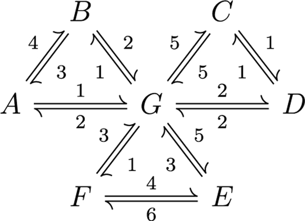
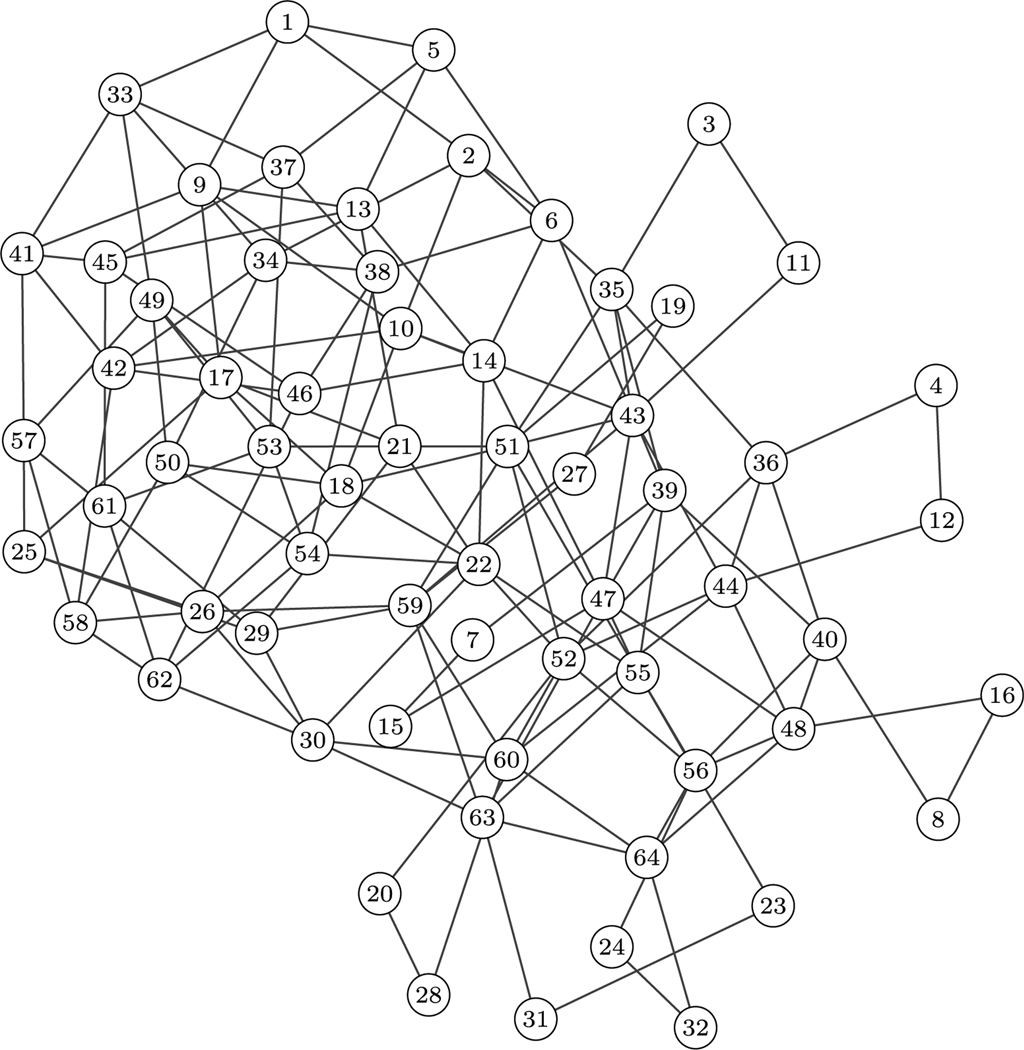
Since ${\mathbb{\text{N}}}^3$ is a small network, a seven-node network ${\mathbb{\text{N}}}^7$ and a 64-node network ${\mathbb{\text{N}}}^{64}$ were also used to validate CycFlowDec. Networks ${\mathbb{\text{N}}}^7$ and ${\mathbb{\text{N}}}^{64}$ are depicted in Figs. 4 and 5, respectively. Network ${\mathbb{\text{N}}}^{64}$ represents a Markov state model of the Cl⁻/H⁺ antiporter [1,20,21] that largely motivated this work.

Fig. 4.

The seven-node flow network ${\mathbb{\text{N}}}^7$.

Fig. 5.

The 64-node flow network ${\mathbb{\text{N}}}^{64}$. Generated with igraph [10] using the large graph layout algorithm. Edges represent bidirectional flows.

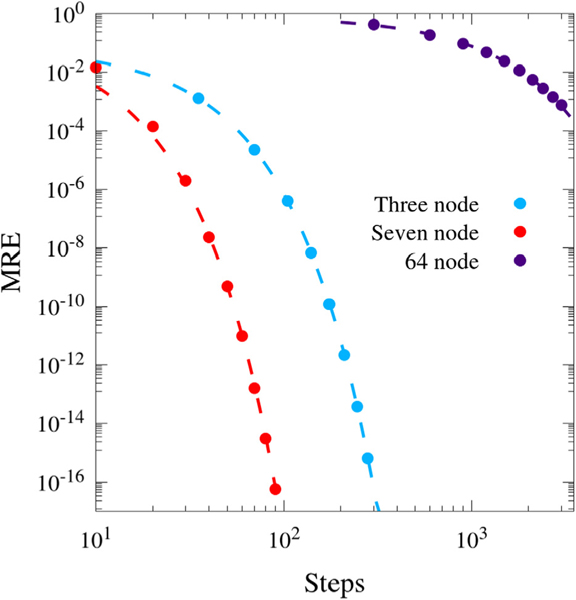
The MRE convergence of the networks is shown in Fig. 6. Intuitively, ${\mathbb{\text{N}}}^{64}$ requires substantially more steps to converge than the other networks; however, ${\mathbb{\text{N}}}^7$ actually converges faster than ${\mathbb{\text{N}}}^3$. This implies that there is another factor affecting convergence besides the number of nodes and edges in the network. It is likely that this third factor is related to the relative flow balance of the network: networks with edge flows of similar magnitudes equilibrate percolation faster than networks with edge flows of highly variant magnitudes. Network ${\mathbb{\text{N}}}^3$ has edge flows that differ by a factor of 10, while the ${\mathbb{\text{N}}}^7$ edge flows are all O(1). Network ${\mathbb{\text{N}}}^{64}$ has edge flows that differ by over 10³. The algorithmic convergence rate is likely a complex function of the number of nodes and edges as well as the flow balance in the network, and warrants further investigation.

Fig. 6.

Log–log plot of MRE vs. steps for ${\mathbb{\text{N}}}^3$, ${\mathbb{\text{N}}}^7$, and ${\mathbb{\text{N}}}^{64}$ using the percolating algorithm with burn-in. Trendlines are of the form y = ae^−bx. Burn-in and minimum contribution tolerance for ${\mathbb{\text{N}}}^3$ and ${\mathbb{\text{N}}}^7$ were N − 2 and zero, respectively. Network ${\mathbb{\text{N}}}^{64}$ used N − 4 and 10⁻⁷. Starting nodes were A, G, and 51 for ${\mathbb{\text{N}}}^3$, ${\mathbb{\text{N}}}^7$, and ${\mathbb{\text{N}}}^{64}$, respectively.

5. Impact

CycFlowDec decomposes closed flow networks into expected simple cycle flows. To the best of our knowledge, no other network analysis tools have been designed to accomplish this task. This tool has a broad potential use given the potentially important role of cyclic flow in closed flow networks in any scientific field involving flow networks, such as chemical reaction networks, communication networks, and more [1,4,5,22–25]. Determining the expected cycle flows in a flow network yields a direct metric for importance of the underlying cycles that constitute network function. This information is especially valuable for quantitatively determining fundamental mechanisms that dictate functional behavior in the network. The example network ${\mathbb{\text{N}}}^{64}$ represents an enzymatic ion transport network of a Cl⁻/H⁺ antiporter, which can be directly analyzed with CycFlowDec [1,20,21]. Future work will expand on this analysis, including the assessment of cycle sensitivity to specific transitions, and applicability to obtain mechanistic insight in the complex biological system.

CycFlowDec is an open source Python module published under the GNU General Public License. This transparency ensures straightforward access to all interested parties and allows further modification of CycFlowDec. Additionally, the lightweight design and simple Python interface enables direct incorporation into general research projects and programs. The simple Python module format is well suited for CycFlowDec due to its wide potential range of applicability for network analysis.

CycFlowDec was designed for the decomposition of close flow networks into simple cycle flows, but it can also be applied to the analysis of open networks with no internal modification. This can be accomplished by defining an effective closed flow network for the open network, where the source nodes are connected to the sink nodes via an intermediate virtual node. Using CycFlowDec to decompose the effective closed network will result in simple cycle flows, some of which include the virtual node. The simple cycles that include the virtual node represent transient path flows, where the transient path is given by removing the virtual node. This additional application of CycFlowDec to open flow networks further increases the range of applicability. For example, CycFlowDec has only been applied to steady state networks involving the Cl⁻/H⁺ antiporter represented by ${\mathbb{\text{N}}}^{64}$, whereas the intermediate, transient state networks could be analyzed using the previously mentioned open network analysis.

6. Conclusions

A novel, efficient algorithm for determining the cyclic flow decomposition of closed networks is presented. The algorithm is incorporated in the open source Python module CycFlowDec. While CycFlowDec was designed for closed networks, it is applicable to open networks by defining an analogous effective closed network where a source and sink flows are sent to a virtual node. CycFlowDec enables more comprehensive analyses of cyclic flow networks, which are present in many fields of science.

Appendix A. Algorithms

The CycFlowDec Python module implements a single efficient, general algorithm based on established Markovian circulation theory [26,27]. The algorithm is a product of three sequential modifications on simpler algorithms that are described first.

A.1. Stochastic algorithm

The first algorithm described is directly obtained from the underlying theory. The pseudocode is provided in algorithm 1. The left stochastic matrix M is calculated using

$$\mathbf{M}[k,j]=e_{j,k}{\left(\sum _{\forall l\in {ℝ}_j}{e}_l\right)}^{-1}\forall j,k\in \mathbb{V},$$ (A.1)

where $\mathbb{\text{V}}$ is the set of all nodes on $\mathbb{\text{N}}$, e_j,k the edge flow from node j to node k, and $\mathbb{\text{E}}$_j is the set of all edges emanating from node j. For ${\mathbb{\text{N}}}^3$ in Fig. 1,

$$\mathbf{M}=\left[\begin{array}{ccc}0& 38/43& 6/9\\ 40/44& 0& 3/9\\ 4/44& 5/43& 0\end{array}\right].$$

Eq. (A.1) is used to calculate M for all algorithms in this work. The stack data structure is appropriate for storing walks, since cycles are always extracted from the end of the walk. Roll(0, 1) rolls a random uniform real number between zero and one that is used to stochastically select the next node in the walk with M. The stack method pop_cycle(k) extracts and returns the encountered cycle starting from node k according to the previously defined procedure. The resulting cycle counts w_c keyed by cycle c are stored in the hash table C, which can be used to calculate cycle flows with Eq. (3).

Algorithm 1:

Stochastic cyclic flow decomposition.

Generate the stochastic matrix M

Initialize an empty stack S

Initialize an empty hash table C

Put a starting node on S

for j 1 to N do

r Roll(0, 1)

for k in rows(M) do

if M[k,S[end]] ≤ r then

break

end if

end for

if k in S then

c = S.pop_cycle(k)

C[c] += 1

else

S.push(k)

end if

end for

A.2. Percolating algorithm

The percolating algorithm extends the stochastic algorithm in the limit of infinite walks emanating from the starting node. In this sense, infinite walks deterministically percolate the network from the starting node, and cycles are extracted and counted as they are encountered. The pseudocode is provided in algorithm 2, for the case that the variables burn and tol (defined in Appendices A.3 and A.4, respectively) are initialized to zero. Instead of explicitly counting the number of occurrences of the simple cycles, the fractional contribution of each cycle with respect to all walks is used for w_c. For example, if 3% of walks go through cycle c at a given iteration, then w_c is incremented by 0.03. The two hash tables H₁ and H₁ keyed by walk stacks are used to alternate the percolation steps and progress the walks. The percolating algorithm takes advantage of the ability to consolidate walks with the same stacks after cycle extraction, allowing the tracking of infinite percolating walks without combinatorial explosion. Similar to the stochastic algorithm, the resulting cycle contributions w_c are stored in hash table C, and can be used to calculate cycle flows with Eq. (3). Both algorithms subsequently described result in C in the same fashion.

A.3. Percolating with burn-in algorithm

The percolating algorithm is subject to initialization bias at earlier iterations, since it takes time for the walks to fully percolate and equilibrate. A straightforward idea to mitigate this issue is to refrain from counting cycles for some number burn of initial iterations. This inclusion of a burn-in with the percolating algorithm is shown in algorithm 2, for the case that the variable tol is initialized to zero.

A.4. Percolating with burn-in and minimum contribution tolerance

For highly connected, large networks, the percolating algorithm will suffer from combinatorial explosion, since the convergence rate decreases linearly with the number of feasible simple cycles. At the cost of maximum achievable accuracy, this issue can be mitigated by only percolating new walk stacks that contribute to the total number of walks above a fractional tolerance tol. This modification is shown in algorithm 2. Walks that contribute below tol but do not result in new walk stacks are still percolated, since they do not increase the total number of walk stacks. Contributions that are not percolated are folded back into the originating walk.

Algorithm 2:

Percolating cyclic flow decomposition with burn-in and minimum contribution tolerance algorithm.

Generate the stochastic matrix M

Initialize an empty hash table H−1

Initialize an empty hash table H1

Initialize an empty hash table C

Initialize a stack S containing a starting node

H−1[S] = 1

b = 1

for j = 1 to N do

for S in H−b.keys() do

Hb S = 0

end for

for S in H−b.keys() do

r = 0

for k in rows(M) do

f = H−b[S] ∗ M[k, S[end]]

Q = S

if H−b S > tol or k in S then

if j > burn and k in S then

c = Q.pop_cycle(k)

C[c] += f

else

Q.push(k)

end if

if Q in Hb.keys() then

Hb[Q] += f

else

Hb[Q] = f

end if

else

r += f

end if

end for

if S in Hb.keys() then

Hb[S] += r

else

Hb[S] = r

end if

end for

b *= −1

end for

Appendix B. Burn-in selection

Fig. B.7.

Semi-log plots of MRE vs. burn-in steps for ${\mathbb{\text{N}}}^3$, ${\mathbb{\text{N}}}^7$, and ${\mathbb{\text{N}}}^{64}$. Total steps were fixed at 150, 50, and 3000 for the three, seven, and 64-node networks, respectively.

Fig. B.8.

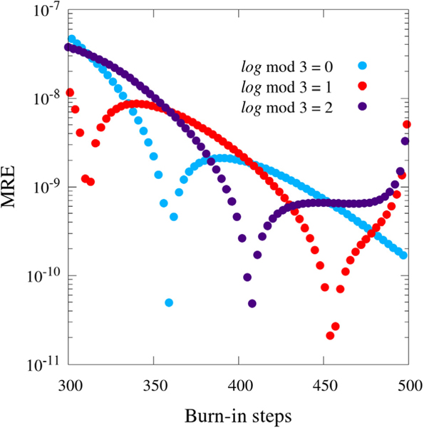
Semi-log plot of MRE vs. burn-in steps for a network analogous to ${\mathbb{\text{N}}}^3$, $\stackrel{\rightharpoonup }{AB}=\stackrel{\rightharpoonup }{BC}=\stackrel{\rightharpoonup }{CA}=40$ and $\stackrel{\rightharpoonup }{AC}=\stackrel{\rightharpoonup }{CB}=\stackrel{\rightharpoonup }{BA}=1$. Total steps were fixed at 500.

The burn-in is a critical component of algorithm efficiency, as demonstrated in Fig. 3. To investigate the effects of burn-in selection, different burn-ins were tested for the same total steps for all three validation networks, shown in Fig. B.7. An interesting pattern arises from this data: all three networks show dual behavior for even and odd burn-in steps. Upon further testing, the behavior is actually dependent on whether the number of cycle logging steps log = N − burn is even or odd. Specifically, even log steps exhibit generally decreasing, lower MRE, while odd log steps exhibit higher MRE with an upturn for log near zero. Network ${\mathbb{\text{N}}}^7$ shows the least difference between even and odd log steps, probably since it contains the most balanced edge flows. A burn-in of N − 2 is slightly higher than N − 4 for ${\mathbb{\text{N}}}^{64}$, probably due to ${\mathbb{\text{N}}}^{64}$ requiring a non-zero minimum contribution tolerance to accelerate its computation.

As it so happens, ${\mathbb{\text{N}}}^3$, ${\mathbb{\text{N}}}^7$, and ${\mathbb{\text{N}}}^{64}$ all have dominant flow cycles of length two. In order to test whether the burn-in behavior was sensitive to this, a network with the same structure as ${\mathbb{\text{N}}}^3$ but with a dominant flow cycle of length three was tested. The result is shown in Fig. B.8. The burn-in behavior appears sensitive to the dominant flow cycle length, as ternary burn-in behavior is observed with the length three cycle dominant network. For complex networks where computational efficiency is a limiting factor, the burn-in behavior should be tested, as no simple, general choice of burn-in is apparent without prior knowledge of cycle flows.

Appendix C. Minimum contribution tolerance selection

Fig. C.9.

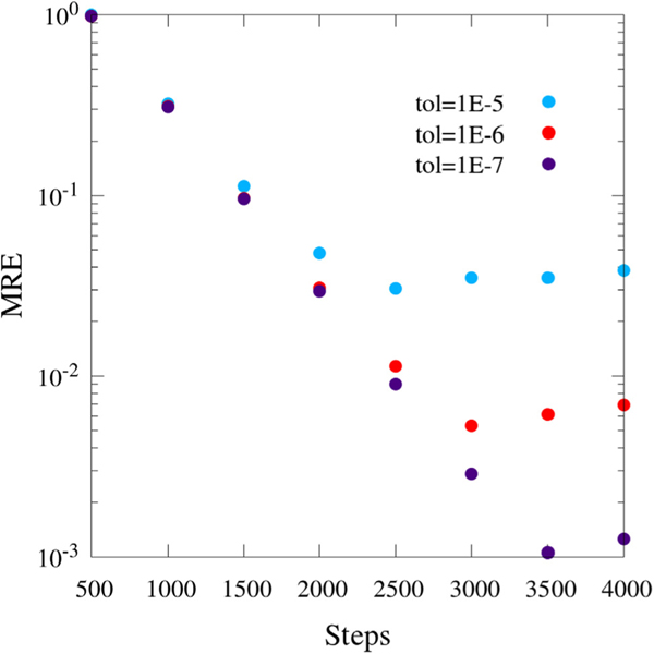
Semi-log plot of MRE vs. steps for different minimum contribution tolerances for ${\mathbb{\text{N}}}^{64}$. Edge flows below 0.1 are omitted from the MRE calculation.

For ${\mathbb{\text{N}}}^{64}$, a minimum contribution tolerance tol is required to permit tractable computation times. The behavior of the cyclic flow network convergence of ${\mathbb{\text{N}}}^{64}$ with respect to tol is shown in Fig. C.9. For all values of tol, the MRE decrease exponentially until a certain step number is reached, and then levels out. This behavior is consistent with the concept that incorporating a minimum contribution tolerance decreases the maximum achievable accuracy of cyclic flow decomposition. Lower MRE is obtainable using lower tolerances, at the cost of increasing computational expense.

References

- [1].Mayes HB, Lee S, White AD, Voth GA, Swanson JM. Multiscale kinetic modeling reveals an ensemble of Cl–/H+ exchange pathways in ClC-ec1 antiporter. J Am Chem Soc 2018;140(5):1793–804. [DOI] [PMC free article] [PubMed] [Google Scholar]
- [2].Rawat W, Wang Z. Deep convolutional neural networks for image classification: A comprehensive review. Neural Comput 2017;29(9):2352–449. [DOI] [PubMed] [Google Scholar]
- [3].Yan Y, Zhang S, Tang J, Wang X. Understanding characteristics in multivariate traffic flow time series from complex network structure. Physica A 2017;477:149–60. [Google Scholar]
- [4].Manik D, Timme M, Witthaut D. Cycle flows and multistability in oscillatory networks. Chaos 2017;27(8):083123. [DOI] [PubMed] [Google Scholar]
- [5].Wang G, Du C, Chen H, Simha R, Rong Y, Xiao Y, Zeng C. Process-based network decomposition reveals backbone motif structure. Proc Natl Acad Sci 2010;107(23):10478–83. [DOI] [PMC free article] [PubMed] [Google Scholar]
- [6].Dantzig G, Fulkerson DR. On the max flow min cut theorem of networks. Linear Inequal Relat Syst 2003;38:225–31. [Google Scholar]
- [7].Froncek D. Cyclic decompositions of complete graphs into spanning trees. Discuss Math Graph Theory 2004;24(2):345–53. [Google Scholar]
- [8].Rosa A. On cyclic decompositions of the complete graph into (4m 2)-gons. Mat-fyz Časopis 1966;16(4):349–52. [Google Scholar]
- [9].Woodhouse FG, Forrow A, Fawcett JB, Dunkel J. Stochastic cycle selection in active flow networks. Proc Natl Acad Sci 2016;113(29):8200–5. [DOI] [PMC free article] [PubMed] [Google Scholar]
- [10].Csardi G, Nepusz T, et al. The igraph software package for complex network research. Int J Complex Syst 2006;1695(5):1–9. [Google Scholar]
- [11].Langfelder P, Horvath S. WGCNA: An R package for weighted correlation network analysis. BMC Bioinformatics 2008;9(1):559. [DOI] [PMC free article] [PubMed] [Google Scholar]
- [12].Handcock MS, Hunter DR, Butts CT, Goodreau SM, Morris M. Statnet: Software tools for the representation, visualization, analysis and simulation of network data. J Stat Softw 2008;24(1):1548. [DOI] [PMC free article] [PubMed] [Google Scholar]
- [13].De Nooy W, Mrvar A, Batagelj V. Exploratory social network analysis with pajek: Revised and expanded edition for updated software, vol. 46. Cambridge University Press; 2018. [Google Scholar]
- [14].Thomas S, Bonchev D. A survey of current software for network analysis in molecular biology. Hum Genom 2010;4(5):353. [DOI] [PMC free article] [PubMed] [Google Scholar]
- [15].Hoops S, Sahle S, Gauges R, Lee C, Pahle J, Simus N, Singhal M, Xu L, Mendes P, Kummer U. COPASI—a complex pathway simulator. Bioinformatics 2006;22(24):3067–74. [DOI] [PubMed] [Google Scholar]
- [16].Banisch R, Conrad ND. Cycle-flow–based module detection in directed recurrence networks. Europhys Lett 2015;108(6):68008. [Google Scholar]
- [17].Banisch R, Conrad N, Schütte C. Reactive flows and unproductive cycles for random walks on complex networks. Eur Phys J Spec Top 2015;224(12):2369–87. [Google Scholar]
- [18].Jia C, Jiang D-Q, Qian M-P, et al. Cycle symmetries and circulation fluctuations for discrete-time and continuous-time Markov chains. Ann Appl Probab 2016;26(4):2454–93. [Google Scholar]
- [19].Fagnola F, Umanita V. Generic quantum Markov semigroups, cycle decomposition and deviation from equilibrium. Infin. Dimens. Anal. Quantum Probab. Relat. Top 2012;15(03):1250016. [Google Scholar]
- [20].Lee S, Swanson JM, Voth GA. Multiscale simulations reveal key aspects of the proton transport mechanism in the ClC-ec1 antiporter. Biophys J 2016;110(6):1334–45. [DOI] [PMC free article] [PubMed] [Google Scholar]
- [21].Lee S, Mayes HB, Swanson JM, Voth GA. The origin of coupled chloride and proton transport in a Cl–/H+ antiporter. J Am Chem Soc 2016;138(45):14923–30. [DOI] [PMC free article] [PubMed] [Google Scholar]
- [22].Hagen L, Keller T, Neely S, DePaula N, Robert-Cooperman C. Crisis communications in the age of social media: A network analysis of Zika-related tweets. Soc Sci Comput Rev 2018;36(5):523–41. [Google Scholar]
- [23].Ding R, Ujang N, bin Hamid H, Abd Manan MS, He Y, Li R, Wu J. Detecting the urban traffic network structure dynamics through the growth and analysis of multi-layer networks. Physica A 2018;503:800–17. [Google Scholar]
- [24].Myers OM, Reyier E, Ahr B, Cook GS. Striped mullet migration patterns in the Indian River Lagoon: A network analysis approach to spatial fisheries management. Mar. Coast. Fish 2020;12(6):423–40. [Google Scholar]
- [25].Iosifidis G, Charette Y, Airoldi EM, Littera G, Tassiulas L, Christakis NA. Cyclic motifs in the Sardex monetary network. Nat Hum Behav 2018;2(11):822–9. [DOI] [PubMed] [Google Scholar]
- [26].Minping Q, Min Q. Circulation for recurrent Markov chains. Z. Wahrscheinlichkeitstheor. Verwandte Geb 1982;59(2):203–10. [Google Scholar]
- [27].Kalpazidou SL. Cycle representations of Markov processes, vol. 28. Springer Science & Business Media; 2007. [Google Scholar]