eLife logoLink to eLife
. 2021 Oct 26;10:e68758. doi: 10.7554/eLife.68758

Infrared molecular fingerprinting of blood-based liquid biopsies for the detection of cancer

Marinus Huber 1,2,, Kosmas V Kepesidis 1,2,, Liudmila Voronina 1, Frank Fleischmann 1, Ernst Fill 2, Jacqueline Hermann 1, Ina Koch 3, Katrin Milger-Kneidinger 4, Thomas Kolben 5, Gerald B Schulz 6, Friedrich Jokisch 6, Jürgen Behr 4, Nadia Harbeck 5, Maximilian Reiser 7, Christian Stief 6, Ferenc Krausz 1,2, Mihaela Zigman 1,2,
Editors: Y M Dennis Lo8, Y M Dennis Lo9
PMCID: PMC8547961  PMID: 34696827

Abstract

Recent omics analyses of human biofluids provide opportunities to probe selected species of biomolecules for disease diagnostics. Fourier-transform infrared (FTIR) spectroscopy investigates the full repertoire of molecular species within a sample at once. Here, we present a multi-institutional study in which we analysed infrared fingerprints of plasma and serum samples from 1639 individuals with different solid tumours and carefully matched symptomatic and non-symptomatic reference individuals. Focusing on breast, bladder, prostate, and lung cancer, we find that infrared molecular fingerprinting is capable of detecting cancer: training a support vector machine algorithm allowed us to obtain binary classification performance in the range of 0.78–0.89 (area under the receiver operating characteristic curve [AUC]), with a clear correlation between AUC and tumour load. Intriguingly, we find that the spectral signatures differ between different cancer types. This study lays the foundation for high-throughput onco-IR-phenotyping of four common cancers, providing a cost-effective, complementary analytical tool for disease recognition.

Research organism: Human

Introduction

To address the ever-growing cancer incidence and mortality rates, effective treatment methods are indispensable (Bray et al., 2018). They rely on detection of the disease at the earliest possible stage to allow antitumour interventions and thus improve survival rates (Bannister and Broggio, 2016; Schiffman et al., 2015). Early detection is therefore a crucial factor in the global fight against cancer.

However, the clinical benefits versus the potential harms and costs of several cancer detection approaches remain controversial (Schiffman et al., 2015). Due to the limited sensitivity and specificity of current medical diagnostics, cancer can either be overlooked (false negatives) or falsely detected (false positives), leading to either delayed interventions or unnecessary, potentially harmful investigations or psychological stress (Srivastava et al., 2019). Hence, there is a high need to complement current medical diagnostics with time- and cost-efficient, non-invasive or minimally invasive methods that could possibly lead to new screening and detection approaches, prior to tissue-biopsy-based molecular profiling or prognosis (Wan et al., 2017).

Molecular analyses of human serum and plasma provide systemic molecular information and enabling novel routes of diagnostics (Amelio et al., 2020; Wan et al., 2017). So far, most liquid biopsies predominantly rely on the analysis of a few pre-selected analytes and biomarkers. Although the emergence of highly sensitive and molecule-specific methods in the fields of proteomics (Geyer et al., 2019; Geyer et al., 2017; Uzozie and Aebersold, 2018), metabolomics (Roig et al., 2017; Xia et al., 2013), and genomics (Abbosh et al., 2017; Han et al., 2017; Otandault et al., 2019) has led to the discovery of thousands of different biomarker candidates, only a few of them have been validated and transferred to the clinic so far (Poste, 2011).

Technological developments of the last decade brought a paradigm change regarding liquid biopsies. Instead of relying on a single molecular marker, recent approaches focus on combining information across a broad range of molecules to investigate changes in molecular patterns and identify disease-specific physiologies. However, the combination of various omics techniques (i.e. multi-omics) still requires complex and target-specific sample preparation as well as elaborate ways of merging different datasets (Hasin et al., 2017; Karczewski and Snyder, 2018; Malone et al., 2020; Yoo et al., 2018). Moreover, increasing the number of analytical methods involved often leads to unfeasibly high costs for broad clinical use.

This is where infrared molecular spectroscopy prevails – it captures signals from all types of molecules in a sample in a single time- and cost-effective measurement in a label-free fashion. When applied to blood serum or plasma samples, infrared spectroscopy provides a so-called infrared molecular fingerprint (IMF) reflecting the chemical composition of a sample, that is, the person’s molecular blood phenotype (Huber et al., 2021). Even though the IMF of a highly complex biofluid such as blood serum and plasma can only partially be traced back to its molecular origin, it may deliver a plethora of information sensitive and specific to the health state of the individual. In a recent longitudinal study, we have shown that defined workflows to collect, store, process, and measure human liquid biopsies lead to reproducible IMFs in healthy, non-symptomatic individuals that are stable over clinically relevant time scales (Huber et al., 2021).

Numerous studies have shown the potential of blood-based IMFs for the detection of cancer, notably brain (Butler et al., 2019; Hands, 2014; Sala et al., 2020b), breast (Backhaus et al., 2010; Elmi et al., 2017; Ghimire et al., 2020; Zelig et al., 2015), bladder (Ollesch et al., 2014), lung (Ollesch et al., 2016), prostate (Medipally et al., 2020), and other cancer entities (Anderson et al., 2020; Ollesch et al., 2014; Sala et al., 2020a), with some of the studies reporting specificities and sensitivities higher than 90% (Anderson et al., 2020; Backhaus et al., 2010; Butler et al., 2019; Ghimire et al., 2020; Medipally et al., 2020; Ollesch et al., 2014). Despite these promising initial results, only a few studies involved more than 75 individuals per group (Anderson et al., 2020). Additionally, the majority of these studies had a high risk of bias due to patient selection applied (Anderson et al., 2020). In fact, it was shown that IMFs are susceptible to external confounding factors, such as those related to sample handling and data collection, as well as to inherent biological variations (e.g. age and gender) unrelated to cancer (Diem, 2018). Furthermore, the differences observed in IMFs may be due to the innate immune response and other concomitant factors (Diem, 2018; Fabian et al., 2005). Thus, the specificity of IMF to a certain cancer must be evaluated by investigation of appropriate, carefully selected reference groups.

Altogether, there is a need for studies that address the issues listed above by (i) systematically investigating the pre-analytical factors (Cameron et al., 2020; Huber et al., 2021), (ii) studying the molecular origin of the infrared fingerprints (Voronina et al., 2021), and (iii) adequately applying machine learning tools with involvement of a sufficient number of participants. To date, the latter requirement has only been met in studies investigating the applicability of infrared fingerprinting to bladder (Ollesch et al., 2014), breast (Backhaus et al., 2010), and brain cancer detection (Butler et al., 2019). In addition to the capacity to detect cancer, whether different cancer entities have sufficiently different infrared spectral signatures to be distinguished from each other has so far not been evaluated.

Our present multi-institutional, multi-disease study addresses the above issues to rigorously assess the feasibility of IMFs for high-throughput detection of four common cancer entities as phenotypes, thus referred to as ‘onco-IR-phenotyping.’ Using Fourier-transform infrared (FTIR) transmission spectroscopy of liquid samples, we measured blood serum and plasma samples from 1927 individuals, among these 161 breast cancer, 118 bladder cancer, 278 prostate cancer, and 214 lung cancer patients, prior to any cancer-related therapy, along with non-symptomatic reference individuals and study participants with diseases and/or benign pathologies of the same organ (i.e. organ-specific symptomatic references). By applying support vector machine (SVM) to train models for binary classification, we obtained detection efficiencies in the range of 0.78–0.89 (area under the receiver operating characteristic [ROC] curve [AUC]), with the detection efficiency strongly correlating with the severity of the disease. The results of this prospectively conducted study suggest that infrared fingerprinting of liquid plasma and serum may offer a means of robust and reliable detection of different types of cancer. Furthermore, we reveal that the spectral signatures attributable to different cancer types differ significantly from each other, which facilitates classification between different states and thus carries a translational potential not previously reported.

Results

Study setup and workflow

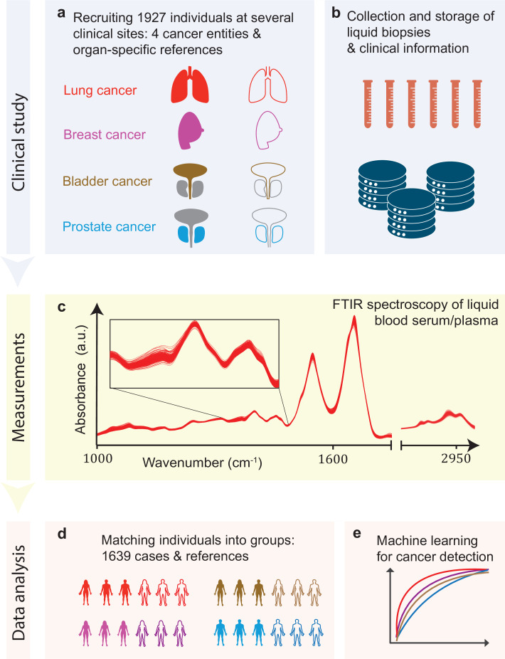
In this study, we tested infrared molecular spectroscopy for medically relevant blood profiling in a prototypical multi-institutional setting, assessing the usefulness of IMFs as a source of complementary information for cancer diagnostics. The study included cohorts of therapy-naïve, lung, prostate, bladder, and breast cancer patients (cases), and organ-specific symptomatic references as well as non-symptomatic reference individuals (Figure 1a, Figure 1—source data 1).

Figure 1. Infrared molecular fingerprinting workflow and clinical study design.

Figure 1.

(a) Cohorts of therapy-naïve, lung, breast, prostate, and bladder cancer patients (cases), and organ-specific symptomatic references as well as non-symptomatic reference individuals were recruited at three different clinical sites – in total, 1927 individuals. (b) Blood samples from all individuals were drawn, and sera and plasma were prepared according to well-defined standard operating procedures. (c) Automated Fourier-transform infrared spectroscopy of liquid bulk sera and plasma were used to obtain IMFs. The displayed IMFs were pre-processed using water correction and normalization (see Methods). (d) For each clinical question studied, the characteristics of the case and the reference cohorts were matched for age, gender, and body mass index (BMI) to avoid patient selection bias. This resulted in total number of 1639 individuals upon matching. (e) Machine learning models were built on training datasets and evaluated on test datasets to separately evaluate the efficiency of classification for each of the four cancer entities.

Figure 1—source data 1. Breakdown of the overall participant pool used within the study.
All the following analyses were carried out on subsets of this participant pool; see also other source data files for further details. When selecting the sub-cohorts, special care was taken to match the case and reference cohorts separately, for each question – according to age, gender, and body mass index (BMI) – in order to avoid possible bias in patient selection.

Blood sera and plasma were collected at several clinical sites according to well-defined standard operating procedures to minimize pre-analytical errors (Figure 1b; Huber et al., 2021). An automated sample delivery system was applied for high-throughput, high-reproducibility, and cost-efficient infrared fingerprinting of liquid sera and plasma of 1927 individuals with an FTIR spectrometer (Figure 1c). Special care was taken to match the characteristics of the case and reference cohorts for each question separately – by age, gender, and body mass index (BMI) – to avoid patient selection bias, although this step reduced the number of individuals analysed within this study to 1639 (Figure 1d). The acquired IMFs were used for training machine learning models to perform binary classification of the samples (Figure 1e) into case and reference groups, allowing the investigation of various clinically relevant questions (see below). Model training was performed by applying SVM algorithm to pre-processed IMFs by splitting the data into train and test sets, employing 10-fold cross-validation, repeated 10-times with randomization. For assessing the classification performance, we evaluated the AUC of the respective ROC curves for the test sets.

Diagnostic performance of infrared molecular fingerprinting for cancer detection

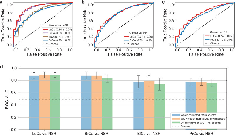
In a first step, we evaluated the diagnostic performance of IMFs obtained from serum samples for the binary classification of each of the four common cancer types individually against matched non-symptomatic reference groups (see Table 1 and Figure 2—source data 1 for details on the characteristics of the individual cohorts). Since our approach produces results in terms of continuous variables (disease likelihood) rather than binary outcomes (disease, non-disease), we use the AUC of the ROC as the main performance metric, and thus take advantage of incorporating information across multiple operating points, not limited to a particular clinical scenario.

Table 1. Detection efficiency for different binary classifications.

Different cancer types were compared to each other, as well as the impact of using different reference groups was analysed. Detailed cohort characteristics can be found in Figure 2—source data 1 (NSR: non-symptomatic references; MR: mixed references; SR: symptomatic references; AUC: area under the receiver operating characteristic curve; *sensitivity and specificity values are obtained by minimizing the distance of the receiver operating characteristic [ROC] curve to the upper-left corner).

Clinical question for binary classification # of Individuals AUC Sensitivity/specificity* sensitivity at95% specificity
Lung cancer vs. NSR 214/193 0.89 ± 0.05 0.86/0.79 0.45
Lung cancer vs. MR 214/208 0.77 ± 0.06 0.72/0.67 0.36
Lung cancer vs. SR 214/143 0.74 ± 0.07 0.67/0.71 0.24
Prostate cancer vs. NSR 278/278 0.78 ± 0.06 0.71/0.71 0.36
Prostate cancer vs. MR 278/278 0.75 ± 0.06 0.71/0.68 0.23
Prostate cancer vs. SR 278/278 0.70 ± 0.06 0.65/0.68 0.20
Breast cancer vs. NSR 161/161 0.88 ± 0.06 0.82/0.81 0.35
Bladder cancer vs. NSR 118/118 0.79 ± 0.09 0.72/0.73 0.23

The highest detection efficiencies in the test sets were obtained for the lung and breast cancer cohort SVM models, with a ROC AUC of 0.89 and 0.88, respectively (Figure 2a). A lower classification performance of 0.79 and 0.78 (ROC AUC) was obtained for the prostate and bladder cancer cohorts, respectively. Table 1 also lists the optimal combination (see Methods) of sensitivity and specificity for all cancer entities. For making our results comparable to other studies and possibly to gold standards in cancer detection, we present lists with sensitivity/specificity pairs (see Table 1). In particular, we present the optimal pairs extracted by minimizing the distance between the ROC curve and the upper-left corner – a standard practice in studies of this type. In addition, we set the specificity to 95% and present the resulting sensitivities.

Figure 2. Diagnostic performance of lung, prostate, bladder, and breast cancer detection based on infrared molecular fingerprints (IMFs) of blood sera.

Receiver operating characteristic (ROC) curves for the binary classification of the test set with support vector machine (SVM) models trained on water-corrected and vector-normalized IMFs. The different cancer entities were tested against (a) non-symptomatic references, (b) mixed references that also include organ-specific symptomatic references, and (c) organ-specific symptomatic references only. Detailed cohort characteristics can be found in Figure 2—source data 1. (d) Area under the receiver operating characteristic curve (AUC) for the test sets according to different spectral pre-processing of the IMFs. The error bars show the standard deviation of the individual results of the cross-validation (LuCa: lung cancer; PrCa: prostate cancer; BrCa: breast cancer; BlCa: bladder cancer; NSR: non-symptomatic references; MR: mixed references; SR: symptomatic references).

Figure 2—source data 1. Characteristics of the matched groups of individuals utilized for the analysis as presented in Table 1, Figures 2 and 3a-c.
Figure 2—source data 2. Zipped folder with trained machine learning models and application instructions.
Figure 2—source data 3. Potential impact of clinical site to classification performance.

Figure 2.

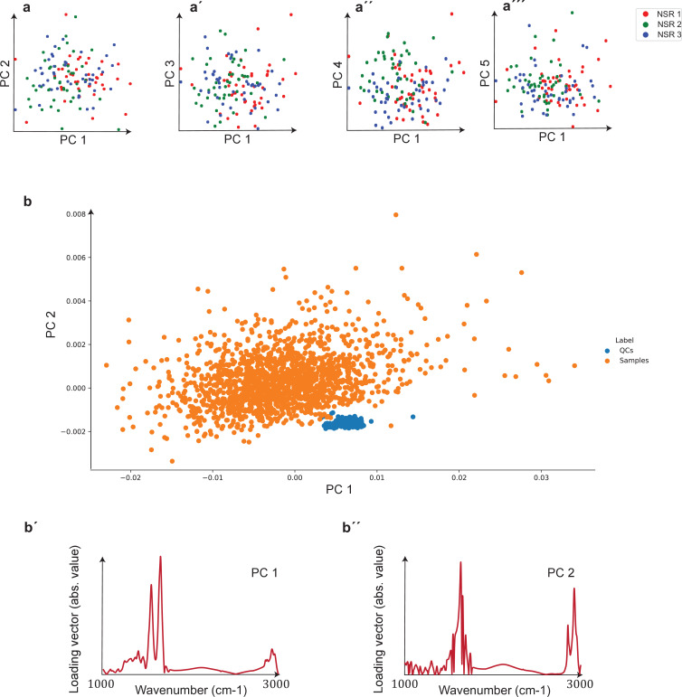
Figure 2—figure supplement 1. Unsupervised comparison between data from the three clinical sites as well as quality control (QC) analysis of measurements.

Figure 2—figure supplement 1.

(a–a′′′) Principal component analysis (PCA) of samples of non-symptomatic healthy individuals collected from three different clinical sites. Plots depict the first five principal components, which correspond to 95% of the explained variance. The three groups are statistically matched in terms of age, gender, and body mass index (BMI). Cohort characteristics are given in Figure 2—figure supplement 1—source data 1. (b) PCA plot of biological samples and QCs. The two first principal components included in the plot correspond to 93% of the explained variance. (b′, b′′) Loading vectors for the two principal components shown in (b).
Figure 2—figure supplement 1—source data 1. Characteristics of the matched groups utilized for the analysis presented in Figure 2—figure supplement 1.
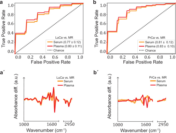
Figure 2—figure supplement 2. Performance comparison of serum- and plasma-based fingerprints for cancer detection.

Figure 2—figure supplement 2.

Receiver operating characteristic (ROC) curves for (a) lung cancer (LuCa) and (b) prostate cancer (PrCa) vs. mixed references (MR). Differential fingerprints (a′, b′) for the same comparisons as above. The characteristics of the cohort used for this analysis are given in Figure 2—figure supplement 2—source data 1.
Figure 2—figure supplement 2—source data 1. Characteristics of the matched groups utilized for the analysis presented in Figure 2—figure supplement 2.

In clinical practice, however, patients may suffer from pathologies that affect the same organ as the cancer under scrutiny. Therefore – in a second step, we tested the capability of IMFs to classify cancer, when organ-specific comorbidities (e.g. chronic obstructive pulmonary disease [COPD] in the lung cancer cohort) and organ-specific benign conditions (e.g. hamartoma of the lung in the lung cancer cohort or benign prostate hyperplasia [BPH] in the prostate cancer cohort – see Figure 1—source data 1 for details) were added to the reference group. In this case, the detection efficiency decreased significantly, from 0.89 to 0.77, for lung cancer and slightly, from 0.79 to 0.75, for prostate cancer (Figure 2b). If the reference group contained only organ-specific symptomatic references, the detection efficiency was reduced further, to 0.74 for lung cancer and 0.70 for prostate cancer (Figure 2c).

To test whether sample collection, handling, and storage have a potential influence on classification results, we examined data from matched, non-symptomatic, healthy individuals from the three major clinics using principal component analysis (PCA). Considering the first five principal components (responsible for 95% of the explained variance), we could not observe any clustering effect related to data from different clinics (Figure 2—figure supplement 1). However, potential bias due to the above-mentioned influences cannot be fully excluded at the present stage. To this end, samples at different clinical sites are being collected to form a large independent test dataset, specifically designed to allow us evaluate the effects of clinical covariates – as well as measurement-related ones – relevant for the proposed IMF-based medical assay. One typically obtains a different AUC by using different control groups, collected at different sites (Figure 2—source data 3). These variations have many potential causes, including measurement-related effects, differences in sample handling, unobserved differences between the clinical populations recruited at different clinical sites, and of course the size of the training sets used for model training, which can significantly affect the model performance. Although important, it is currently not feasible to rigorously disentangle these effects. Furthermore, we investigated the influence of different pre-processing of the IMFs on the classification results and reassuringly found that these are not significantly affected by the applied pre-processing (Figure 2d). Model diagnostics yielded no signs of overfitting as we added different layers of pre-processing into the pipeline (see Methods for details). Since water-corrected and vector-normalized spectra typically resulted in slightly higher AUCs but still low overfitting, this pre-processing was kept in all other analyses.

It is generally known that blood serum and blood plasma provide largely overlapping molecular information, and both can be used as a basis for many further investigations. The extent to which this also applies to infrared fingerprinting has not been extensively studied. In a previous comparative study, we were able to show that healthy phenotypes can be better identified on the basis of serum (Huber et al., 2021).

Here we compare the diagnostic performance of IMFs from serum and plasma collected from the same individuals for the detection of lung and prostate cancer compared to non-symptomatic and symptomatic organ-specific references. Given that plasma samples were only available for a subset of the lung and prostate cohorts, the results for serum slightly deviate from those presented above due to the different cohort characteristics (Figure 2—figure supplement 2—source data 1). The detection efficiency based on IMFs from plasma samples was 3% higher in the case of lung cancer and 2% higher in the case of prostate cancer than the same analysis based on IMFs from serum samples. In both cases, the difference in AUC was only of low significance. It is noteworthy that the corresponding ROC curves show similar behaviour (Figure 2—figure supplement 2). These results suggest that either plasma or serum samples could in principle be used for detection of these cancer conditions. However, for carefully assessing whether (i) the same amount of information is contained in both biofluids and (ii) whether this information is encoded in a similar way across the entire spectra requires yet an additional dedicated study with higher sample numbers.

Investigation of cancer-specific infrared signatures

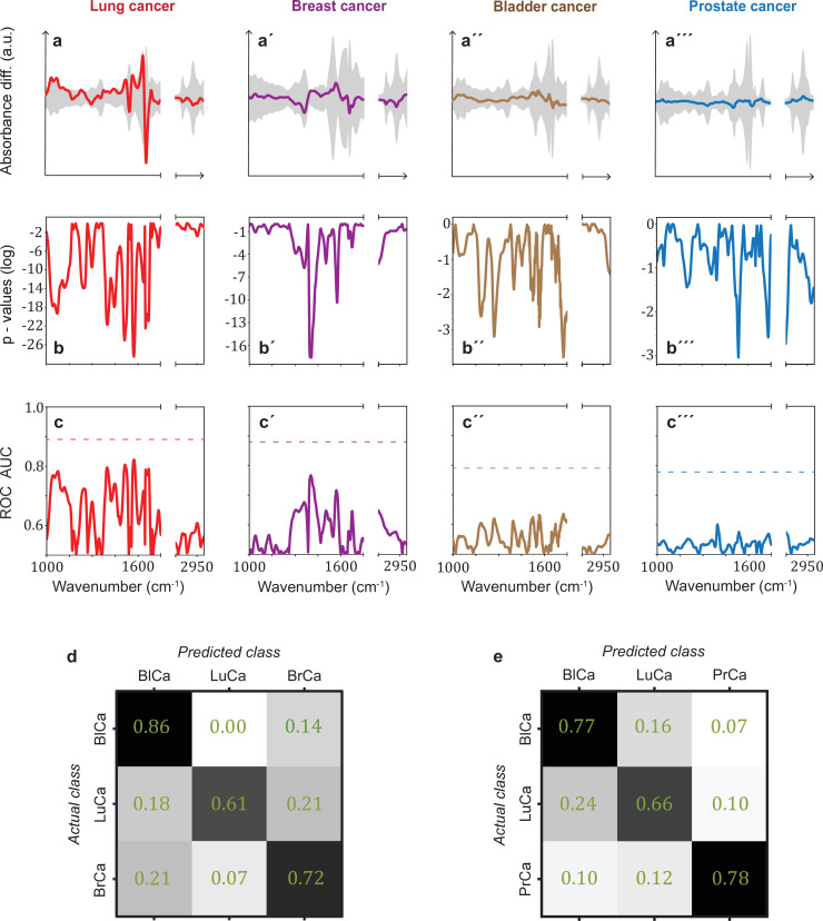
In many clinical settings, a simple binary classification may not be sufficient; instead, a simple, quick, and reliable test that indicates a specific cancer or disease is preferred. To investigate the possible existence of cancer-specific IMFs (or onco-IR-phenotypes), we first examined and compared the spectral signatures that are relevant for distinguishing cancer cases from non-symptomatic references. For this purpose, we evaluated the differential fingerprints (defined as the difference between the mean IMF of the case cohort and that of the reference cohort), determined the two-tailed p-value of Student’s t-test, and calculated the AUC per wavenumber using the U statistic of a Mann–Whitney U test (see Methods) for all cohorts (Figure 3a–c). The obtained patterns differed significantly for all four cancer entities.

Figure 3. Infrared spectral signatures of lung, prostate, bladder, and breast cancer.

(a-a''') Differential fingerprints (standard deviations of the reference cohorts are displayed as grey areas), (b-b''') two-tailed p-value of Student’s t-test, and (c-c''') area under the receiver operating characteristic curve (AUC) per wavenumber (extracted by application of Mann–Whitney U test) compared to the AUC of the combined model (dashed horizontal lines). Confusion matrix summarizing the per-class accuracies of multiclass classification of (d) lung, bladder, and breast cancer (matched female cohort) with overall model accuracy of 0.73 ± 0.11, and (e) lung, bladder, and prostate cancer (matched male cohort) with overall model accuracy of 0.74 ± 0.13. Detailed cohort characteristics can be found in Figure 3—source data 1. Chance level for the three-class classification corresponds to 0.33 (LuCa: lung cancer; PrCa: prostate cancer; BrCa: breast cancer; BlCa: bladder cancer).

Figure 3—source data 1. Characteristics of the matched groups utilized for the analysis presented in Figure 3d and e.

Figure 3.

Figure 3—figure supplement 1. Comparison of signatures from different organ-specific pathologies.

Figure 3—figure supplement 1.

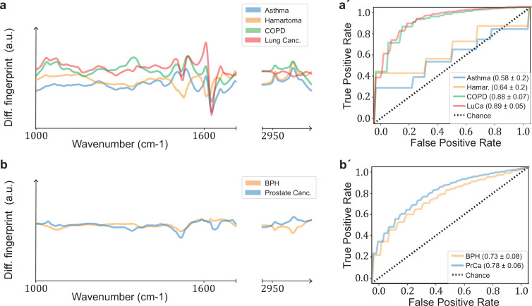
Differential fingerprints for (a) lung-related conditions (asthma, lung hamartoma, chronic obstructive pulmonary disease [COPD], lung cancer) and (b) prostate-related pathologies (benign prostate hyperplasia [BPH], prostate cancer). Receiver operating characteristic (ROC) curves for (a′) lung and (b′) prostate pathologies. All comparisons are against non-symptomatic references. The characteristics of the cohort used for this analysis are given in Figure 3—figure supplement 1—source data 1.
Figure 3—figure supplement 1—source data 1. Characteristics of the matched groups utilized for the analysis presented in Figure 3—figure supplement 1.

It is noteworthy that for lung and breast cancer the magnitude of the differential fingerprint compared to the variation of the IMFs of the reference group (grey area in Figure 3a) is more pronounced than for bladder and prostate cancer. This is also reflected in the p-values (Figure 3b), reaching many orders of magnitude lower levels for the former cancer entities, and higher spectrally resolved AUCs (Figure 3c). Compared to evaluation based on the entire spectral range, spectral containment significantly reduces detection efficiency for all cancer entities, although the reduction is smaller for lung and breast cancer. For these two cancer entities, classification based on a few selected spectral regions is possible. By contrast, for prostate and bladder cancer, the cancer-relevant information appears to be distributed over the entire spectral range and a high classification rate relies on the entire spectral range accessible.

The fact that the cancer entities studied here have different spectral signatures raises the question of whether it is possible to get first indication of the type of cancer detected, which can become relevant, for example, if the primary origin of a cancer type is unknown. Therefore, we performed a multiclass classification aiming to distinguish between lung, bladder, and breast cancer for a matched female cohort (Figure 3d) and between lung, bladder, and prostate cancer for a matched male cohort (Figure 3e). Note that the number of included cancer cases had to be significantly reduced in multiclass classification, as compared to the binary classification, in order to preserve balanced cohort characteristics. Details on this are given in Figure 3—source data 1. Overall, the classification accuracy was 73% and 74%, respectively. These findings suggest that primary tumours evolving in different organs indeed induce differing changes in the overall molecular composition of blood sera – as reflected in differing spectral signatures – and thus offering potential for cancer stratification in future. However, due to the small dataset, these findings need to be verified with larger, independent cohorts.

Often, a patient may reveal symptoms suggestive of a certain cancer entity (e.g. lung cancer), but same time also symptoms indicative of additional further diseases or benign conditions. Therefore, we tested the ability of infrared fingerprinting to detect signatures that would be specific to lung and prostate cancer in comparison to organ-specific (benign) diseases in each case. To this end, we evaluated the differential fingerprints of the different organ-specific symptomatic references compared to non-symptomatic individuals and compared these signatures to the cancer-related IMFs, respectively (Figure 3—figure supplement 1). We found that the differential fingerprint for asthma and lung hamartoma clearly differs from the ones obtained for lung cancer and COPD. However, the differential fingerprints of the latter two diseases, although distinguishable, exhibit strong similarities in their main spectral features. This explains why the presence of COPD in the reference group lowers the detection efficiency of lung cancer (Figure 2a vs. Figure 2b). In contrast, the differential fingerprints of BPH and prostate cancer differ considerably. Consequently, BPH in the reference group does not strongly affect the detection efficacy of prostate cancer.

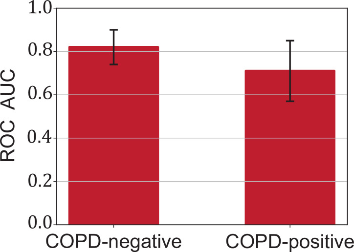
Lung cancer is often accompanied by COPD, and the previous analysis showed that the differential fingerprint of COPD and lung cancer exhibits similarities. Thus, we investigated whether infrared fingerprinting could possibly identify any infrared signals specific only to lung cancer (and not to COPD). Towards that end, we separated individuals from the above analysis into sub-cohorts with subjects negative and positive for COPD. We found that the detection of lung cancer was less efficient when the reference cohort contained only COPD-positive individuals (Figure 4—figure supplement 1,). Both conditions (lung cancer and COPD) are often accompanied by an inflammatory response. Considering that the spectral signatures relevant for cancer detection are based on typical molecular changes that also occur in inflammatory conditions (Voronina et al., 2021), the presence of COPD likely masks, at least in part, cancer-relevant signals.

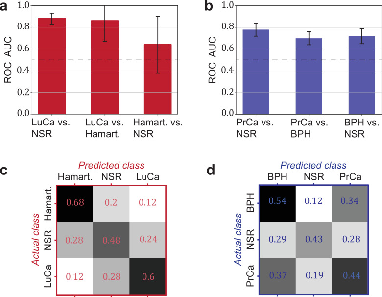
Another relevant question is whether a distinction between cancer and corresponding organ-specific benign pathologies can be made. Here, we evaluated to what extent this was possible for lung and prostate cancer. In both cases, we observed that the cancer detection was only moderately higher against a group of non-symptomatic individuals as compared to a group of patients with a benign condition (lung hamartoma and BPH, respectively; see Figure 4a and b).

Figure 4. Detection efficiency of benign conditions and multiclass classification.

(a) Pairwise classification performance results between lung cancer (LuCa), hamartoma (Hamart.) and non-symptomatic reference group (NSR) with overall model accuracy of 0.46 ± 0.18, and (b) pairwise classification performance between prostate cancer (PrCa), benign prostate hyperplasia (BPH), and NSR with overall model accuracy of 0.43 ± 0.06. The error bars show the standard deviation of the individual results of the cross-validation. Confusion matrix summarizing the per-class accuracies of multiclass classification in (c) the LuCa cohort and (d) the PrCa cohort. The characteristics of the cohort used for this analysis are given in Figure 4—source data 1. Chance level for the three-class classification corresponds to 0.33.

Figure 4—source data 1. Characteristics of the matched groups utilized for the analysis presented in Figure 4.

Figure 4.

Figure 4—figure supplement 1. Influence of chronic obstructive pulmonary disease (COPD) in lung cancer (LuCa) detection.

Figure 4—figure supplement 1.

Classification performance of LuCa vs. mixed references as a function of the COPD status. The characteristics of the cohort used for this analysis are given in Figure 4—figure supplement 1—source data 1.
Figure 4—figure supplement 1—source data 1. Characteristics of the matched groups utilized for the analysis presented in Figure 4—figure supplement 1.

Finally, we explored the possibility of creating multiclass classification models to simultaneously discriminate between multiple groups: cancer patients, individuals with benign conditions, and non-symptomatic reference subjects (Figure 4c and d). In both cases, the classification accuracy was well above chance. Although the accuracy may not yet be sufficient for clinical use, these accuracies may significantly improve with more samples available for training.

Dependence of cancer detection performance on tumour progression

Challenges for cancer detection include the enormous biological and clinical complexity of cancer, and detection is further complicated by the significant intratumour heterogeneity (McGranahan and Swanton, 2017) as well as by the impact of the tumour microenvironment (Boothby and Rickert, 2017). To evaluate whether the blood-based IMFs are sensitive to tumour progression, we first investigated whether the binary classification efficiency depends on tumour size, characterized in terms of clinical TNM staging (Amin et al., 2017).

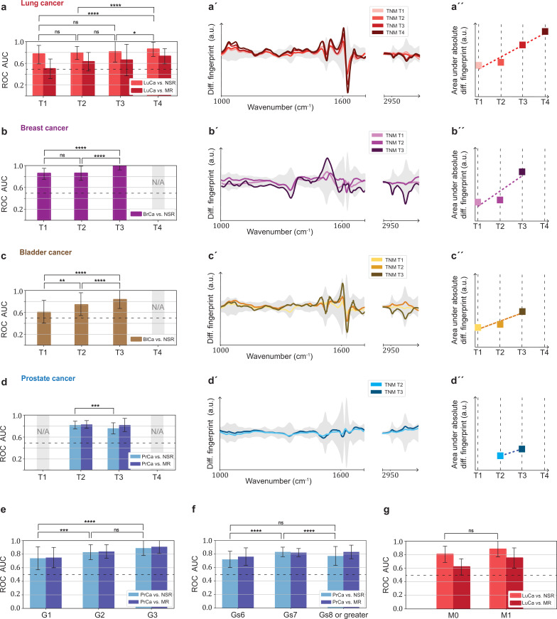
In general, we observe that the classification efficiency exhibits a positive correlation with tumour size or tumour grade. In the case of lung cancer, when compared to the non-symptomatic references, the classification efficiency for T4 tumours is (in terms of AUC) 9% higher than that for T1 tumours (Figure 5a). Also, for breast and bladder cancer, a significantly higher detection efficiency for T3 tumours was observed. This is also reflected by the fact that a more pronounced differential fingerprint can be found in these cancers in higher T classes (Figure 5a–c). Although the absolute (integrated) deviation – between the cases and the matched references – increases for all four cancer phenotypes, the spectral features are partly different for the different T stages. This could be due to the fact that, due to the moderate number of individuals considered, the actual onco-IR-phenotype is masked by biological variability, or that the heterogeneity of tumour growth leads to different molecular changes and thus to different IMFs.

Figure 5. Efficiency of binary classification and infrared spectral changes in dependence of tumour progression.

(a–d) Binary classification performance of lung, breast, bladder, and prostate cancer against references as a function of T-classification (of TNM-staging). (a′–d′) Differential fingerprints in relation with the tumour size (TNM class T) for all four cancer entities. (a′′–d′′) Area under the absolute differential fingerprints in relation with the tumour size for all dour cancer entities. The y-axes of the diagrams in the panels (a'–d') and (a''–d'') each have the same linear scaling, thus directly comparable. (e) Classification performance of prostate cancer versus references as a function of tumour grade score. (f) Classification performance of prostate cancer as a function of the Gleason score (Gs). (g) Classification performance of lung cancer versus references as a function of the metastasis status. The detailed cohort breakdown and classification results are given as Figure 5—source data 1, Figure 5—source data 2, Figure 5—source data 3, Figure 5—source data 4. Some cohorts did not include sufficient number of participants so that a reliable machine learning model could not be built and were therefore not evaluated. LuCa: lung cancer; PrCa: prostate cancer; BrCa: breast cancer; BlCa: bladder cancer; NSR: non-symptomatic references; MR: mixed references; n.s.: not significant; *p<10–2; **p<10–3; ***p<10–4; ****p<10–5; The error bars show the standard deviation of the individual results of the cross-validation.

Figure 5—source data 1. Characteristics of the matched groups utilized for the analysis presented in Figure 5a-d, a'-d' and a"-d".
Figure 5—source data 2. Characteristics of the matched groups utilized for the analysis presented in Figure 5e.
Figure 5—source data 3. Characteristics of the matched groups utilized for the analysis presented in Figure 5f.
Figure 5—source data 4. Characteristics of the matched groups utilized for the analysis presented in Figure 5e.

Figure 5.

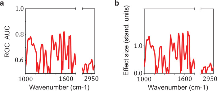
Figure 5—figure supplement 1. Relation between the effect size and the area under the receiver operating characteristic curve (AUC) per wavenumber.

Figure 5—figure supplement 1.

Comparison between (a) the AUC per wavenumber and (b) the effect size per wavenumber. The effect size is defined as the standardized difference between the sample means of cases and references, also known as Cohen’s d. The AUC per wavenumber is calculated using the U statistic of Mann–Whitney U test by the relation AUC = U/(n1 * n2). This example was performed for the comparison lung cancer (LuCa) vs. non-symptomatic references (NSR).

In contrast, prostate cancer with higher T stage shows neither a significantly better AUC nor a more pronounced differential fingerprint (Figure 5d). Instead, the detection efficiency does increase significantly with tumour grade score (Amin et al., 2017; Figure 5e). A strong correlation between the AUC and Gleason score (Figure 5f) could also not be observed.

Finally, the size of the lung cohort allowed us to also investigate the possible effect of metastasis (TNM M1) on the IMFs and their classification performance. As expected from our previous findings, higher AUCs (although not statistically significantly higher) were found in the cohort of locally advanced and metastatic lung cancer as compared to cohort of non-metastatic cancer patients only (Figure 5g).

Overall, we observe a consistent pattern in agreement with the hypothesis that the signal utilized by the learning algorithm increases with more progressed disease stage (either larger tumour volume, metastatic spread, or tumour grade score). This suggests that the information retrieved from the measured differences between the IMFs of cases and references is connected to tumour-related molecular changes. These changes may be due to larger tumour load leaving a more extensive footprint on the composition of peripheral blood, or to the fact that tumour progression could have caused a higher systemic response, or to a combination of both. While the correlation between AUC and tumour size was most evident for lung, breast, and bladder cancer, spectral signatures relevant for prostate cancer detection were more strongly connected to the tumour grade score. It is important to note, however, that the observed relation – between the spectrum of the disease and classification efficiency – is not conclusively proven by the current analysis, but only suggested.

Discussion

We demonstrated the feasibility of blood-based IMF to detect lung, breast, bladder, and prostate cancer with good efficiency. Although previous smaller studies have yielded fairly high classification efficiencies (Backhaus et al., 2010; Elmi et al., 2017; Ghimire et al., 2020; Medipally et al., 2020; Ollesch et al., 2016; Ollesch et al., 2014; Zelig et al., 2015), they were either based on low number of participants or might have been affected by confounding factors. Here we provided a rigorous multi-institutional study setup with more than 100 individuals in each case and reference group, 1927 individuals in total, with all case and reference cohorts matched for major confounding factors (n = 1639 individuals upon matching). In addition, we observed that visible infrared spectral signatures correlate with tumour stage, suggesting that the IMFs are significantly affected not only by the presence of tumours but also by the progression of the disease. Furthermore, similar cancer detection efficiencies were achieved with IMFs obtained from blood serum and plasma. This not only confirms the robustness of the results, but also reveals that the method is applicable to both biofluids.

This study provides strong indications that blood-based IMF patterns can be utilized to identify various cancer entities, and therefore provides a foundation for a possible future in vitro diagnostic method. However, IMF-based testing is still at the evaluation stage of essay development, and further steps have to be undertaken to evaluate the clinical utility, reliability, and robustness of the IMF approach (Ignatiadis et al., 2021).

First, the machine learning models built within this work will have to be tested with fully independent sample sets. Although the study was designed to account for and minimize the effect of confounding factors, we are aware that these cannot be fully excluded, especially considering that machine learning algorithms are susceptible to them (Zhao et al., 2020). To this end, we freeze the current machine learning models, each trained on the data of the entire cohorts of the current study (Figure 2—source data 2), and will apply them to a consecutively prospective sample collection to better rule out potential confounders.

Second, it needs to be studied in more detail whether IMFs pick up molecular patterns that are specific to a primary disease process or, more generally, to any secondary inflammatory response. At the current stage, both options seem possible as altered immune responses are also known as primary disease drivers in the context of cancer and may affect genome instability, cancer cell proliferation, anti-apoptotic signalling, angiogenesis, and, last but not least, cancer cell dissemination (Hanahan and Weinberg, 2011). This link to systemic effects makes it still difficult to distinguish cancer-specific IMFs (onco-IR-phenotypes) from comorbidities with a strong immune signature (like COPD) in humans in vivo. Nevertheless, we did obtain distinct spectral patterns for all four common cancer entities (Figure 3b) indicating different, potentially disease-specific molecular alterations of the IMFs. These changes are likely to be linked to cancer-induced changes since classification accuracy is higher with more advanced cancer stages, which is also reflected in more pronounced differential fingerprints with larger tumour size.

To gain deeper understanding of the specificity of observed spectral changes to the disease patterns studied, it is helpful to investigate their molecular origin. In this context, we do not consider the approach of assigning spectral positions/features to characteristic vibrational modes of functional molecular entities most appropriate. Although widely used in the IR community, due to the very many molecular assignments possible for each spectral position, unambiguous statements of molecular changes herein are not feasible. Instead, a much deeper analysis is required, as recently revealed by Sangster et al., 2006; Voronina et al., 2021. The latter work involves combination of infrared spectroscopy and quantitative mass spectrometry on the part of the lung cancer sample set used in the current study as well, identifying the molecular origin of the differential infrared fingerprints. These can be partially explained by a characteristic change of proteins that are known to also change due to systemic inflammatory signals. Thereby we highlight the need for further biochemical investigations into the molecular origin of the observed spectral signatures, generally required in the field to address this question conclusively.

In-depth information about the molecular origin of the observed spectral disease patterns will help identify the clinical setting(s) where infrared fingerprinting can make largest contributions to cancer care (e.g. screening, diagnosis, prognosis, treatment monitoring, or surveillance). The specificity of spectral signatures to cancer, along with the obtained sensitivity and specificity in the binary classification (Table 1), will influence whether the approach may best complement primary diagnostics, be possibly suited for screening, or even be used for molecular profiling and prognostication. When further validated, blood-based IMFs could aid residing medical challenges: More specifically, it may complement radiological and clinical chemistry examinations prior to invasive tissue biopsies. Given less than 60 μl of sample are required, sample preparation time and effort are negligible, and measurement time is within minutes, the approach may be well suited for high-throughput screening or provide additional information for clinical decision process. Thus, minimally invasive IMF cancer detection could integratively help raise the rate of pre-metastatic cancer detection in clinical testing. However, further detailed research (e.g. as performed for an FTIR-based blood serum test for brain tumour; Gray et al., 2018) is needed to identify an appropriate clinical setting in which the proposed test can be used with the greatest benefit (in terms of cost-effectiveness and clinical utility).

Moreover, given the recent evidence of high within-person stability of IMFs over time (Huber et al., 2021), serial longitudinal liquid biopsies and infrared fingerprinting of respective samples could eliminate between-person variability by self-referencing and thereby facilitate even more efficient and possibly earlier cancer detection. Once (i) a precise clinical setting is defined and (ii) large-scale, stratified clinical studies controlled for comorbidities can be realized, a systematic, direct comparison to established diagnostics will become feasible and the full potential of infrared fingerprinting can be quantitatively assessed.

For further improvements in the accuracy of the envisioned medical assay, the IR fingerprinting methodology needs to be improved in parallel. Molecular specificity is inherently limited in IR spectroscopy due to the spectral overlap of absorption bands of individual molecules. This might be tackled by chemical pre-fractionation (Hughes et al., 2014; Petrich et al., 2009; Voronina et al., 2021) or by combining IR spectroscopy to methods like liquid chromatography. However, such a pre-fractioning, but also IR fingerprinting itself, would benefit even more from increased spectroscopic sensitivity. Sensitivity of the current commercially available FTIR spectrometer is however limited to detection of highly abundant molecules. Recent developments in infrared spectroscopy demonstrate the possibility to increase the detectable molecular dynamic range to five orders of magnitude (Pupeza et al., 2020) and therefore have the potential to improve the efficiency of infrared fingerprinting.

In summary, infrared fingerprinting reveals the potential for effective detection and distinction of various common cancer types already at its current stage and implementation. Future developments, in terms of instrumentation as well as methodology, have the potential to further improve the detection efficiency. This study presents a general high-throughput and cost-effective framework, and along this, highlights the possibility for extending infrared fingerprinting to other disease entities.

Methods

Study design

The objective of this study was to evaluate whether infrared molecular fingerprinting of human blood serum and plasma from patients, reference individuals, and healthy persons has any capacity to detect cancer, specifically targeting detection of four common cancer entities (lung, breast, bladder, and prostate cancer). A statistical power calculation for the sample size was performed prior to the study and is included in the study protocol. Based on preliminary results, it was determined that with a sample size of 200 cases and 200 controls, the detection power in terms of AUC can be estimated within a marginal error of 0.054. Therefore, the aim was to include more than 200 cases for each cancer type. However, upon matching (see also below), it was not always possible to include 200 individuals per group for all analyses of this study. In the analyses where the sample size of 200 individuals per group could not be reached, the uncertainty obtained increased accordingly (as seen in the obtained errors and error bars). The full sample size calculation is available on request from the corresponding authors.

The multi-institutional study on lung, breast, bladder, and prostate cancer also includes subjects with corresponding benign pathologies in the same organs as well as non-symptomatic subjects. Participants provided written informed consent for the study under research study protocol #17-141 and broad consent under research study protocol #17-182, both of which were approved by the Ethics Committee of the Ludwig-Maximillian-University (LMU) of Munich. Our study complies with all relevant ethical regulations and was conducted according to Good Clinical Practice (ICH-GCP) and the principles of the Declaration of Helsinki. The clinical trial is registered (ID DRKS00013217) at the German Clinical Trails Register (DRKS). The following clinical centres were involved in subject recruitment and sample collections of the prospective clinical study: Department of Internal Medicine V for Pneumology, Urology Clinic, Breast Center, Department of Obstetrics and Gynecology, and Comprehensive Cancer Centre Munich (CCLMU), all affiliated with the LMU. The Asklepios Lung Clinic (Gauting), affiliated to the Comprehensive Pneumology Centre (CPC) Munich, and the German Centre for Lung Research, DZL, were further study sites in the Munich region, Germany. In total, blood samples from 1927 individuals were collected and measured (see below). The full breakdown of all participants is listed in Figure 1—source data 1.

From the existing dataset, the recorded IMFs were selected for further analysis according to the following criteria:

  • Only data from cancer patients with clinically confirmed carcinoma of lung, prostate, bladder, or breast prior to any cancer-related therapy were considered.

  • Healthy references were non-symptomatic individuals not suffering from any cancer-related disease nor being under any medical treatment.

  • Symptomatic references included patients with COPD or pulmonary hamartoma for lung cancer, and BPH patients for prostate cancer.

From this pre-selected dataset, a further subset was created for each binary classification examined (e.g. lung cancer vs. non-symptomatic references). This selection was done using statistical matching (see below) in such a way that it provides a balanced distribution of gender, age, and BMI. This was to ensure that there is no bias towards any of these factors within the analysis of machine learning. The selection step reduced the number of analysed samples to 1639. It is important to note that given that we have performed evaluations addressing more than one main question, depending on some types of questions, some control samples are appropriately used as matched references for multiple questions.

A full breakdown of all included participants (sample pool) along with the breakdown for each of the investigated binary classification is provided as source data files.

Statistical matching

Achieving covariate balance between cases and references is an important procedure in observational studies for neutralizing the effect of confounding factors and limiting the bias in the results. In this work, we deploy optimal pair matching using the Mahalanobis distance within propensity score callipers (Rosenbaum, 2010). The implementation was done in R (v. 3.5.1). In evaluations where pair matching was not sufficient, optimal matching with multiple references was performed instead.

Sample collection and storage

Blood samples were collected, processed, and stored according to the same standard operating procedures at each clinical site. Blood draws were all performed using Safety-Multifly needles of at least 21 G (Sarstedt) and collected with 4.9 ml or 7.5 ml serum and plasma Monovettes (Sarstedt). For the blood clotting process to take place, the tubes were stored upright for at least 20 min and then centrifuged at 2000 g for 10 min at 20°C. The supernatant was carefully aliquoted into 0.5 ml fractions and frozen at –80°C within 5 hr after collection. Samples were transported to the analysis site on dry ice and again stored at –80°C until sample preparation.

Sample preparation and FTIR measurements

In advance of the FTIR measurements, one 0.5 ml aliquot per serum or plasma sample was thawed in a water bath at 4°C and again centrifuged for 10 min at 2000 g. The supernatant was distributed into the measurement tubes (50 µl per tube) and refrozen at –80°C. All the FTIR measurements were performed upon two freeze-thaw cycles.

The samples were mostly measured in the order in which they arrived at the measurement site. As sample collection and delivery is to some extent a stochastic process (both cases and references were continuously collected over the entire period), no additional randomization of the measurement order was performed.

The samples were aliquoted and measured in blinded fashion, that is, the person performing the measurements did not know about any clinical information about the samples. The spectroscopic measurements were performed in liquid phase with an automated FTIR device (MIRA-Analyzer, micro-biolytics GmbH) with a flow-through transmission cuvette (CaF2 with ~8 µm path length). The spectra were acquired with a resolution of 4 cm–1 in a spectral range between 950 cm–1 and 3050 cm–1. A water reference spectrum was recorded after each sample measurement to reconstruct the IR absorption spectra. Each measurement sequence usually contained up to 40 samples, resulting in measurement times of up to 3 hr. After each measurement batch, the instrument was carefully cleaned and re-qualified according to the manufacturer’s recommendations.

To track experimental errors over extended time periods (Sangster et al., 2006), a measurement of quality control serum (pooled human serum, BioWest, Nuaillé, France) was performed after every five samples. The spectra of the QC samples were also used to evaluate the measurement error. We found in a previous study that the measurement error is small when compared to the between-person biological variability of human serum IMFs (Huber et al., 2021). A relevant analysis comparing the variability between biological samples and QCs is presented in Figure 2—figure supplement 1b-b". In addition, the results obtained on a subset from plasma and serum samples from the same individuals were similar, indicating that no technical variance or device variation affected the measurement results. Thus, individual samples were not measured as replicates.

Outlier detection

If an air bubble was present during the measurement, this was immediately noticeable by saturation of the detector. In such cases, the measurement was considered faulty and another aliquot of the sample was measured. After the entire dataset was collected, we performed an additional outlier removal. For this, we used the method of Local Outlier Factor (LOF), as implemented in Scikit-Learn (v. 0.23.2) (Pedregosa et al., 2011). LOF is based on k-nearest neighbours and is appropriate for (moderately) high-dimensional data. LOF succeeds in removing samples with spectral anomalies such as abnormally low absorbance or contamination signatures. Using this procedure, a total of 28 spectra were removed from the dataset.

Pre-processing of infrared absorption spectra

Negative absorption, which occurs if the liquid sample contains less water than the reference (pure water), was corrected for by a previously described approach (Yang et al., 2015). It is known from measurements of dried serum or plasma that there is no significant absorption in the wavenumber region 2000–2300 cm–1, resulting in a flat absorption baseline. We used this fact as a criterion for adding to each spectrum a previously measured water absorption spectrum (as provided in Figure 2—source data 2) to account for the missing water in the sample measurement and minimize the average slope in this region in order to obtain a flat baseline. All spectra were truncated to 1000–3000 cm–1 and the ‘silent region,’ between 1750 cm–1 and 2800 cm–1, was removed. Finally, all spectra were normalized using Euclidean (L2) norm. The calculation of the second derivative of the normalized spectra was included in some cases as an additional (optional) pre-processing step.

Machine learning and classification

To derive classification models, we used Scikit-Learn (Pedregosa et al., 2011; v. 0.23.2), an open-source machine learning framework in Python (v.3.7.6). We trained various binary classification as well as multiclass classification models using linear SVM. Performance evaluation was carried out using repeated stratified k-fold cross-validation and its visualization using the notion of the ROC curve for binary problems and the confusion matrix for multiclass classification. The results of the cross-validation are reported in terms of descriptive statistics, that is, the mean value of the resulting AUC distribution and its standard deviation. The calculation of optimal pair of sensitivity and specificity is done by minimizing the distance of the ROC curve to the upper-left corner.

Statistical analysis

For statistically comparing two groups of spectra (i.e. cases, references), we followed three approaches. First, we calculated the ‘differential fingerprint,’ defined as the sample mean of the cases minus the sample mean of the reference group. We plot this quantity contrasted against the standard deviation of the reference group for obtaining a visual understanding of which wavenumbers are potentially useful for distinguishing/classifying the two populations. Such a graph serves as a visual representation of what is known as the ‘effect size,’ which can be obtained by standardizing the differential fingerprint and, as shown in Figure 5—figure supplement 1, has an evident relation to the AUC per wavenumber. Secondly, we performed t-test (testing the hypothesis that two populations have equal means) for extracting two-tailed p-values per wavenumber. As a last step, we make use of Mann–Whitney U test (also known as Wilcoxon rank-sum test) for extracting the U statistic and calculating the AUC per wavenumber by the relation AUC = U/(n1*n2), where n1 and n2 are the sizes of the two groups.

Acknowledgements

We thank Prof. Dr. Gabriele Multhoff, Dr. Stefan Jungblut, Katja Leitner, Dr. Sigrid Auweter, Daniel Meyer, Beate Rank, Sabine Witzens, Christina Mihm, Sabine Eiselen, Tarek Eissa, and Dr. Incinur Zellhuber for their help with this study. In particular, we wish to acknowledge the efforts of many individuals who participated as volunteers in the clinical study reported here. We also thank the Asklepios Biobank for Lung Diseases, member of the German Center for Lung Research (DZL), for providing clinical samples and data.

Funding Statement

No external funding was received for this work.

Contributor Information

Mihaela Zigman, Email: mihaela.zigman@mpq.mpg.de.

Y M Dennis Lo, The Chinese University of Hong Kong, Hong Kong.

Y M Dennis Lo, The Chinese University of Hong Kong, Hong Kong.

Additional information

Competing interests

No competing interests declared.

No competing interests declared.

Author contributions

Conceptualization, Data curation, Formal analysis, Investigation, Methodology, Validation, Visualization, Writing – original draft, Writing – review and editing.

Conceptualization, Formal analysis, Investigation, Methodology, Validation, Visualization, Writing – original draft, Writing – review and editing.

Data curation, Formal analysis, Methodology, Writing – review and editing.

Data curation, Investigation, Methodology, Supervision.

Conceptualization, Formal analysis, Investigation, Methodology.

Methodology, Project administration, Supervision, Validation.

Data curation, Investigation, Resources, Validation.

Resources.

Resources, Supervision.

Investigation.

Investigation.

Conceptualization, Resources, Supervision, Writing – review and editing.

Conceptualization, Resources, Supervision, Writing – review and editing.

Conceptualization, Resources, Writing – review and editing.

Conceptualization, Resources, Writing – review and editing.

Conceptualization, Funding acquisition, Investigation, Methodology, Resources, Supervision, Visualization, Writing – review and editing.

Conceptualization, Formal analysis, Funding acquisition, Investigation, Methodology, Project administration, Resources, Supervision, Visualization, Writing – original draft, Writing – review and editing.

Ethics

Clinical trial registration DRKS00013217.

The multi-institutional study on lung, breast, bladder and prostate cancer includes cancer patients as well as subjects with corresponding benign pathologies in the same organs as well as non-symptomatic subjects. Participants provided written informed consent for the study under research study protocol #17-141 and broad consent under research study protocol #17-182, both of which were approved by the Ethics Committee of the Ludwig-Maximillian-University (LMU) of Munich. Our study complies with all relevant ethical regulations, and was conducted according to Good Clinical Practice (ICH-GCP) and the principles of the Declaration of Helsinki. The clinical trial is registered (ID DRKS00013217) at the German Clinical Trails Register (DRKS).

Additional files

Transparent reporting form

Data availability

The datasets analysed within the scope of the study cannot be published publicly due to privacy regulations under the General Data Protection Regulation (EU) 2016/679. The raw data includes clinical data from patients, including textual clinical notes and contain information that could potentially compromise subjects' privacy or consent, and therefore cannot be shared. However, the trained machine learning models for the binary classification of bladder, breast, prostate, and lung cancer are provided within Figure 2—source data 4, along with description and code for importing them in a python script. The custom code used for the production of the results presented in this manuscript is stored in a persistent repository at the Leibniz Supercomputing Center of the Bavarian Academy of Sciences and Humanities (LRZ), located in Garching, Germany. The entire code can only be shared upon reasonable request, as its correct use depends heavily on the settings of the experimental setup and the measuring device and should therefore be clarified with the authors.

References

  1. Abbosh C, Birkbak NJ, Wilson GA, Jamal-Hanjani M, Constantin T, Salari R, Le Quesne J, Moore DA, Veeriah S, Rosenthal R, Marafioti T, Kirkizlar E, Watkins TBK, McGranahan N, Ward S, Martinson L, Riley J, Fraioli F, Al Bakir M, Grönroos E, Zambrana F, Endozo R, Bi WL, Fennessy FM, Sponer N, Johnson D, Laycock J, Shafi S, Czyzewska-Khan J, Rowan A, Chambers T, Matthews N, Turajlic S, Hiley C, Lee SM, Forster MD, Ahmad T, Falzon M, Borg E, Lawrence D, Hayward M, Kolvekar S, Panagiotopoulos N, Janes SM, Thakrar R, Ahmed A, Blackhall F, Summers Y, Hafez D, Naik A, Ganguly A, Kareht S, Shah R, Joseph L, Marie Quinn A, Crosbie PA, Naidu B, Middleton G, Langman G, Trotter S, Nicolson M, Remmen H, Kerr K, Chetty M, Gomersall L, Fennell DA, Nakas A, Rathinam S, Anand G, Khan S, Russell P, Ezhil V, Ismail B, Irvin-Sellers M, Prakash V, Lester JF, Kornaszewska M, Attanoos R, Adams H, Davies H, Oukrif D, Akarca AU, Hartley JA, Lowe HL, Lock S, Iles N, Bell H, Ngai Y, Elgar G, Szallasi Z, Schwarz RF, Herrero J, Stewart A, Quezada SA, Peggs KS, Van Loo P, Dive C, Lin CJ, Rabinowitz M, Aerts HJWL, Hackshaw A, Shaw JA, Zimmermann BG, TRACERx consortium. PEACE consortium. Swanton C. Phylogenetic CTDNA analysis depicts early-stage lung cancer evolution. Nature. 2017;545:446–451. doi: 10.1038/nature22364. [DOI] [PMC free article] [PubMed] [Google Scholar]
  2. Amelio I, Bertolo R, Bove P, Buonomo OC, Candi E, Chiocchi M, Cipriani C, Di Daniele N, Ganini C, Juhl H, Mauriello A, Marani C, Marshall J, Montanaro M, Palmieri G, Piacentini M, Sica G, Tesauro M, Rovella V, Tisone G, Shi Y, Wang Y, Melino G. Liquid biopsies and cancer omics. Cell Death Discovery. 2020;6:131. doi: 10.1038/s41420-020-00373-0. [DOI] [PMC free article] [PubMed] [Google Scholar]
  3. Amin MB, Edge SB, Greene FL, Byrd DR, Brookland RK, Washington MK, Gershenwald JE, Compton CC, Hess KR, Sullivan DC, Jessup JM, Brierley JD, Gaspar LE, Schilsky RL, Balch CM, Winchester DP, Asare EA, Madera M, Gress DM, Meyer LR. AJCC Cancer Staging Manual. Springer; 2017. [DOI] [Google Scholar]
  4. Anderson DJ, Anderson RG, Moug SJ, Baker MJ. Liquid biopsy for cancer diagnosis using vibrational spectroscopy: systematic review. BJS Open. 2020;4:554–562. doi: 10.1002/bjs5.50289. [DOI] [PMC free article] [PubMed] [Google Scholar]
  5. Backhaus J, Mueller R, Formanski N, Szlama N, Meerpohl HG, Eidt M, Bugert P. Diagnosis of breast cancer with infrared spectroscopy from serum samples. Vibrational Spectroscopy. 2010;52:173–177. doi: 10.1016/j.vibspec.2010.01.013. [DOI] [Google Scholar]
  6. Bannister N, Broggio J. Cancer Survival by Stage at Diagnosis for England (Experimental Statistics) Office for National Statistics; 2016. [Google Scholar]
  7. Boothby M, Rickert RC. Metabolic Regulation of the Immune Humoral Response. Immunity. 2017;46:743–755. doi: 10.1016/j.immuni.2017.04.009. [DOI] [PMC free article] [PubMed] [Google Scholar]
  8. Bray F, Ferlay J, Soerjomataram I, Siegel RL, Torre LA, Jemal A. Global cancer statistics 2018: GLOBOCAN estimates of incidence and mortality worldwide for 36 cancers in 185 countries. CA. 2018;68:394–424. doi: 10.3322/caac.21492. [DOI] [PubMed] [Google Scholar]
  9. Butler HJ, Brennan PM, Cameron JM, Finlayson D, Hegarty MG, Jenkinson MD, Palmer DS, Smith BR, Baker MJ. Development of high-throughput ATR-FTIR technology for rapid triage of brain cancer. Nature Communications. 2019;10:4501. doi: 10.1038/s41467-019-12527-5. [DOI] [PMC free article] [PubMed] [Google Scholar]
  10. Cameron JM, Butler HJ, Anderson DJ, Christie L, Confield L, Spalding KE, Finlayson D, Murray S, Panni Z, Rinaldi C, Sala A, Theakstone AG, Baker MJ. Exploring pre-analytical factors for the optimisation of serum diagnostics: Progressing the clinical utility of ATR-FTIR spectroscopy. Vibrational Spectroscopy. 2020;109:103092. doi: 10.1016/j.vibspec.2020.103092. [DOI] [Google Scholar]
  11. Diem M. Comments on recent reports on infrared spectral detection of disease markers in blood components. Journal of Biophotonics. 2018;11:e201800064. doi: 10.1002/jbio.201800064. [DOI] [PubMed] [Google Scholar]
  12. Elmi F, Movaghar AF, Elmi MM, Alinezhad H, Nikbakhsh N. Application of FT-IR spectroscopy on breast cancer serum analysis. Spectrochim Acta Part A Mol Biomol Spectrosc. 2017;187:87–91. doi: 10.1016/j.saa.2017.06.021. [DOI] [PubMed] [Google Scholar]
  13. Fabian H, Lasch P, Naumann D. Analysis of biofluids in aqueous environment based on mid-infrared spectroscopy. Journal of Biomedical Optics. 2005;10:031103. doi: 10.1117/1.1917844. [DOI] [PubMed] [Google Scholar]
  14. Geyer PE, Holdt LM, Teupser D, Mann M. Revisiting biomarker discovery by plasma proteomics. Molecular Systems Biology. 2017;13:942. doi: 10.15252/msb.20156297. [DOI] [PMC free article] [PubMed] [Google Scholar]
  15. Geyer PE, Voytik E, Treit P, Doll S, Kleinhempel A, Niu L, Müller JB, Buchholtz M, Bader JM, Teupser D, Holdt LM, Mann M. Plasma Proteome Profiling to detect and avoid sample‐related biases in biomarker studies. EMBO Molecular Medicine. 2019;11:1–12. doi: 10.15252/emmm.201910427. [DOI] [PMC free article] [PubMed] [Google Scholar]
  16. Ghimire H, Garlapati C, Janssen EAM, Krishnamurti U, Qin G, Aneja R, Perera AGU. Protein Conformational Changes in Breast Cancer Sera Using Infrared Spectroscopic Analysis. Cancers. 2020;12:1708. doi: 10.3390/cancers12071708. [DOI] [PMC free article] [PubMed] [Google Scholar]
  17. Gray E, Butler HJ, Board R, Brennan PM, Chalmers AJ, Dawson T, Goodden J, Hamilton W, Hegarty MG, James A, Jenkinson MD, Kernick D, Lekka E, Livermore LJ, Mills SJ, O’Neill K, Palmer DS, Vaqas B, Baker MJ. Health economic evaluation of a serum-based blood test for brain tumour diagnosis: Exploration of two clinical scenarios. BMJ Open. 2018;8:e017593. doi: 10.1136/bmjopen-2017-017593. [DOI] [PMC free article] [PubMed] [Google Scholar]
  18. Han X, Wang J, Sun Y. Circulating Tumor DNA as Biomarkers for Cancer Detection. Genomics, Proteomics & Bioinformatics. 2017;15:59–72. doi: 10.1016/j.gpb.2016.12.004. [DOI] [PMC free article] [PubMed] [Google Scholar]
  19. Hanahan D, Weinberg RA. Hallmarks of Cancer: The Next Generation. Cell. 2011;144:646–674. doi: 10.1016/j.cell.2011.02.013. [DOI] [PubMed] [Google Scholar]
  20. Hands JR. Attenuated Total Reflection Fourier Transform Infrared (ATR-FTIR) spectral discrimination of brain tumour severity from serum samples. Journal of Biophotonics. 2014;7:189–199. doi: 10.1002/jbio.201300149. [DOI] [PubMed] [Google Scholar]
  21. Hasin Y, Seldin M, Lusis A. Multi-omics approaches to disease. Genome Biology. 2017;18:83. doi: 10.1186/s13059-017-1215-1. [DOI] [PMC free article] [PubMed] [Google Scholar]
  22. Huber M, Kepesidis K, Voronina L, Božić M, Trubetskov M, Harbeck N, Krausz F, Žigman M. Stability of person-specific blood-based infrared molecular fingerprints opens up prospects for health monitoring. Nature Communications. 2021;12:1511. doi: 10.1038/s41467-021-21668-5. [DOI] [PMC free article] [PubMed] [Google Scholar]
  23. Hughes C, Brown M, Clemens G, Henderson A, Monjardez G, Clarke NW, Gardner P. Assessing the challenges of Fourier transform infrared spectroscopic analysis of blood serum. Journal of Biophotonics. 2014;7:180–188. doi: 10.1002/jbio.201300167. [DOI] [PubMed] [Google Scholar]
  24. Ignatiadis M, Sledge GW, Jeffrey SS. Liquid biopsy enters the clinic — implementation issues and future challenges. Nature Reviews. Clinical Oncology. 2021;18:297–312. doi: 10.1038/s41571-020-00457-x. [DOI] [PubMed] [Google Scholar]
  25. Karczewski KJ, Snyder MP. Integrative omics for health and disease. Nature Reviews. Genetics. 2018;19:299–310. doi: 10.1038/nrg.2018.4. [DOI] [PMC free article] [PubMed] [Google Scholar]
  26. Malone ER, Oliva M, Sabatini PJB, Stockley TL, Siu LL. Molecular profiling for precision cancer therapies. Genome Medicine. 2020;12:8. doi: 10.1186/s13073-019-0703-1. [DOI] [PMC free article] [PubMed] [Google Scholar]
  27. McGranahan N, Swanton C. Clonal Heterogeneity and Tumor Evolution: Past, Present, and the Future. Cell. 2017;168:613–628. doi: 10.1016/j.cell.2017.01.018. [DOI] [PubMed] [Google Scholar]
  28. Medipally DKR, Cullen D, Untereiner V, Sockalingum GD, Maguire A, Nguyen TNQ, Bryant J, Noone E, Bradshaw S, Finn M, Dunne M, Shannon AM, Armstrong J, Meade AD, Lyng FM. Vibrational spectroscopy of liquid biopsies for prostate cancer diagnosis. Therapeutic Advances in Medical Oncology. 2020;12:175883592091849. doi: 10.1177/1758835920918499. [DOI] [PMC free article] [PubMed] [Google Scholar]
  29. Ollesch J, Heinze M, Heise HM, Behrens T, Brüning T, Gerwert K. It’s in your blood: spectral biomarker candidates for urinary bladder cancer from automated FTIR spectroscopy. Journal of Biophotonics. 2014;7:210–221. doi: 10.1002/jbio.201300163. [DOI] [PubMed] [Google Scholar]
  30. Ollesch J, Theegarten D, Altmayer M, Darwiche K, Hager T, Stamatis G, Gerwert K. An infrared spectroscopic blood test for non-small cell lung carcinoma and subtyping into pulmonary squamous cell carcinoma or adenocarcinoma. Biomedical Spectroscopy and Imaging. 2016;5:129–144. doi: 10.3233/BSI-160144. [DOI] [Google Scholar]
  31. Otandault A, Anker P, Al Amir Dache Z, Guillaumon V, Meddeb R, Pastor B, Pisareva E, Sanchez C, Tanos R, Tousch G, Schwarzenbach H, Thierry AR. Recent advances in circulating nucleic acids in oncology. Annals of Oncology. 2019;30:374–384. doi: 10.1093/annonc/mdz031. [DOI] [PubMed] [Google Scholar]
  32. Pedregosa F, Weiss R, Brucher M. Scikit-learn: Machine Learning in Python. Journal of Machine Learning Research. 2011;12:2825–2830. doi: 10.1007/s13398-014-0173-7.2. [DOI] [Google Scholar]
  33. Petrich W, Lewandrowski KB, Muhlestein JB, Hammond MEH, Januzzi JL, Lewandrowski EL, Pearson RR, Dolenko B, Früh J, Haass M, Hirschl MM, Köhler W, Mischler R, Möcks J, Ordóñez–Llanos J, Quarder O, Somorjai R, Staib A, Sylvén C, Werner G, Zerback R. Potential of mid-infrared spectroscopy to aid the triage of patients with acute chest pain. The Analyst. 2009;134:1092. doi: 10.1039/b820923e. [DOI] [PubMed] [Google Scholar]
  34. Poste G. Bring on the biomarkers. Nature. 2011;469:156–157. doi: 10.1038/469156a. [DOI] [PubMed] [Google Scholar]
  35. Pupeza I, Huber M, Trubetskov M, Schweinberger W, Hussain SA, Hofer C, Fritsch K, Poetzlberger M, Vamos L, Fill E, Amotchkina T, Kepesidis K, Apolonski A, Karpowicz N, Pervak V, Pronin O, Fleischmann F, Azzeer A, Žigman M, Krausz F. Field-resolved infrared spectroscopy of biological systems. Nature. 2020;577:52–59. doi: 10.1038/s41586-019-1850-7. [DOI] [PubMed] [Google Scholar]
  36. Roig B, Rodríguez-Balada M, Samino S, Ewf L, Guaita-Esteruelas S, Gomes AR, Correig X, Borràs J, Yanes O, Gumà J. Metabolomics reveals novel blood plasma biomarkers associated to the BRCA1-mutated phenotype of human breast cancer. Scientific Reports. 2017;7:17831. doi: 10.1038/s41598-017-17897-8. [DOI] [PMC free article] [PubMed] [Google Scholar]
  37. Rosenbaum PR. Design of Observational Studies, Springer Series in Statistics. Springer; 2010. [DOI] [Google Scholar]
  38. Sala A, Anderson DJ, Brennan PM, Butler HJ, Cameron JM, Jenkinson MD, Rinaldi C, Theakstone AG, Baker MJ. Biofluid diagnostics by FTIR spectroscopy: A platform technology for cancer detection. Cancer Letters. 2020a;477:122–130. doi: 10.1016/j.canlet.2020.02.020. [DOI] [PubMed] [Google Scholar]
  39. Sala A, Spalding KE, Ashton KM, Board R, Butler HJ, Dawson TP, Harris DA, Hughes CS, Jenkins CA, Jenkinson MD, Palmer DS, Smith BR, Thornton CA, Baker MJ. Rapid analysis of disease state in liquid human serum combining infrared spectroscopy and “digital drying. Journal of Biophotonics. 2020b;13:118. doi: 10.1002/jbio.202000118. [DOI] [PubMed] [Google Scholar]
  40. Sangster T, Major H, Plumb R, Wilson AJ, Wilson ID. A pragmatic and readily implemented quality control strategy for HPLC-MS and GC-MS-based metabonomic analysis. The Analyst. 2006;131:1075–1078. doi: 10.1039/b604498k. [DOI] [PubMed] [Google Scholar]
  41. Schiffman JD, Fisher PG, Gibbs P. Early Detection of Cancer: Past, Present, and Future. Am Soc Clin Oncol Educ B. 2015;10:57–65. doi: 10.14694/EdBook_AM.2015.35.57. [DOI] [PubMed] [Google Scholar]
  42. Srivastava S, Koay EJ, Borowsky AD, De Marzo AM, Ghosh S, Wagner PD, Kramer BS. Cancer overdiagnosis: a biological challenge and clinical dilemma. Nature Reviews. Cancer. 2019;19:349–358. doi: 10.1038/s41568-019-0142-8. [DOI] [PMC free article] [PubMed] [Google Scholar]
  43. Uzozie AC, Aebersold R. Advancing translational research and precision medicine with targeted proteomics. Journal of Proteomics. 2018;189:1–10. doi: 10.1016/j.jprot.2018.02.021. [DOI] [PubMed] [Google Scholar]
  44. Voronina L, Leonardo C, Mueller‐Reif JB, Geyer PE, Huber M, Trubetskov M, Kepesidis K, Behr J, Mann M, Krausz F, Žigman M. Molecular Origin of Blood‐Based Infrared Spectroscopic Fingerprints**. Angew Chemie Int Ed Anie. 2021;60:17060–17069. doi: 10.1002/anie.202103272. [DOI] [PMC free article] [PubMed] [Google Scholar]
  45. Wan JCM, Massie C, Garcia-Corbacho J, Mouliere F, Brenton JD, Caldas C, Pacey S, Baird R, Rosenfeld N. Liquid biopsies come of age: Towards implementation of circulating tumour dna. Nature Reviews. Cancer. 2017;17:223–238. doi: 10.1038/nrc.2017.7. [DOI] [PubMed] [Google Scholar]
  46. Xia J, Broadhurst DI, Wilson M, Wishart DS. Translational biomarker discovery in clinical metabolomics: An introductory tutorial. Metabolomics. 2013;9:280–299. doi: 10.1007/s11306-012-0482-9. [DOI] [PMC free article] [PubMed] [Google Scholar]
  47. Yang H, Yang S, Kong J, Dong A, Yu S. Obtaining information about protein secondary structures in aqueous solution using Fourier transform IR spectroscopy. Nature Protocols. 2015;10:382–396. doi: 10.1038/nprot.2015.024. [DOI] [PubMed] [Google Scholar]
  48. Yoo BC, Kim KH, Woo SM, Myung JK. Clinical multi-omics strategies for the effective cancer management. Journal of Proteomics. 2018;188:97–106. doi: 10.1016/j.jprot.2017.08.010. [DOI] [PubMed] [Google Scholar]
  49. Zelig U, Barlev E, Bar O, Gross I, Flomen F, Mordechai S, Kapelushnik J, Nathan I, Kashtan H, Wasserberg N, Madhala-Givon O. Early detection of breast cancer using total biochemical analysis of peripheral blood components: a preliminary study. BMC Cancer. 2015;15:408. doi: 10.1186/s12885-015-1414-7. [DOI] [PMC free article] [PubMed] [Google Scholar]
  50. Zhao Q, Adeli E, Pohl KM. Training confounder-free deep learning models for medical applications. Nature Communications. 2020;11:6010. doi: 10.1038/s41467-020-19784-9. [DOI] [PMC free article] [PubMed] [Google Scholar]

Decision letter

Editor: Y M Dennis Lo1

In the interests of transparency, eLife publishes the most substantive revision requests and the accompanying author responses.

Acceptance summary:

This manuscript describes the use of infrared molecular fingerprinting for the detection of multiple types of cancer. The spectral differences between different cancer types have further expanded the diagnostic potential. This work has laid the foundation for future developments in this area.

Decision letter after peer review:

Thank you for submitting your article "Infrared molecular fingerprinting of blood-based liquid biopsies for the detection of cancer" for consideration by eLife. Your article has been reviewed by 2 peer reviewers, and the evaluation has been overseen by myself as a Reviewing Editor. The reviewers have opted to remain anonymous.

The reviewers have discussed their reviews with one another, and the Reviewing Editor has drafted this to help you prepare a revised submission.

Essential revisions:

1. The paper would benefit from further transparency on the numbers of patients used in the analysis. The authors state that they collected blood (serum and plasma) from 1927 individuals with cancer, symptomatic controls and healthy controls in the abstract. In depth reading and analysis of the paper shows that this dataset is then reduced to 1611 and that plasma samples are only available from a subset of lung and prostate cohorts. They should also explain why 316 patients were removed from the dataset. Further analysis of the supplementary highlights that some discriminations are performed with only 28 samples per disease type for instance the multi cancer discrimination in the female group between bladder, lung and breast and in the male group between bladder lung and prostate there are only 90 per group. As a major claim of the paper is the fact that the authors can distinguish between these types of tumours and that the signatures are significantly different enough a discussion on whether the size of the dataset analysed is sufficient to have that conclusion should be presented. Also the major class within the dataset analysed is the number of subjects with no related conditions (n=635) so essentially the non-symptomatic healthy controls. As the authors in the introduction highlight the fact that there is a need to adequately apply machine learning tools with involvement of a sufficient number of samples and they state that they address this in this paper they should highlight the number of samples involved in each of the analysis they perform or at least discuss the weaknesses that arise. This issue of low sample numbers is an issue in the field and the authors are correct to highlight this in the introduction. The authors state that a power calculation has been performed and is available on request. This should be provided with the paper to show that 28 samples per disease state achieves the required level of significance.

2. The authors utilise an unsupervised PCA based approach to show that there is no difference between the collection sites in supplementary figure 1. However, from experience it is known that a PCA would not show discrimination between the cancers that the authors have analysed. This may be one explanation as to why the authors needed to use an SVM in order to enable the discrimination of the tumour types. To properly enable this conclusion the authors could show the PCA (along with loadings and not just score plots) for the tumour types or perform an SVM on the samples from the three collection sites in order to fully support this conclusion.

3. The authors also state that the pre-processing of the IMFs did not affect the classification result indicating high quality raw data. In order to not mislead a reader is should be noted that what the authors refer to as raw data is not raw data. It is in fact the spectra after a water correction has been performed to correct for negative absorptions. From knowledge the negative absorptions are variable between spectra and it would be interesting for the reader to have a discussion on how often negative absorptions appear in the liquid serum or plasma. Fundamentally the spectra referred to by the authors for subsequent normalisation or 2nd derivatisation have had a correction performed and a such are not raw. In order to fully support this conclusion, it would be interesting to see the impact on the classification accuracy of the raw spectra (the spectra to which the negative absorption has not been applied)

4. Please further expand on what is meant by quality control serum sample – as there a particular serum used for this and what was the procedure for proving quality – do you have a quality test and did any fail at any point?

5. One key objective the study aims to achieve is to improve the specificity of the study by including more suitable control subjects. However, the study still fails to identify which parts of the signal were directly related to the existence of cancer-related molecules. It would be useful for the authors to try to dissect out the most representative cancer signals and to identify the molecules giving rise to those signals.

6. The authors used AUC of ROC curves to reflect the clinical utility of the test. However, for evaluating the usefulness of diagnostic markers, the sensitivities at a specificity of 95% and/or 99% (for screening markers) are frequently used. The presentation of these data would be useful to indicate if the test would be useful in clinical settings.

7. The authors showed that the ROC curves for plasma and serum had similar AUC and concluded that they provided similar infrared information. This point is incorrect. To prove that both plasma and serum can reflect signals from the cancer, the authors need to show that the actual infrared pattern from the plasma and serum are identical.

8. In the discussion, the authors need to discuss:

i. if the current performance of the test is sufficient for clinical use, and how that can assist in the clinical decision process;

ii. how the performance of the test can be improved.

(Merely increasing in the number of test/control subjects is unlikely to lead to a dramatic improvement in the accuracy which makes the test clinically useful.)

Reviewer #1:

The authors carried out a multi-center trial to evaluate the potential clinical use of infrared molecular fingerprinting (IMF) for detecting cancer signatures in the blood. In previous proof-of-principle studies, only small numbers of samples were analyzed and that would be subjected to bias related to preanalytical factors and the demographic difference between the cancer patients and control group.

This study performed a one-to-one match of the cancer patients and the controls, and also included symptomatic subjects with benign conditions as controls. This could much better reflect the clinical utility of the test in a real-world situation.

As the study used machine learning to identify the patterns associated with cancer in blood, it did not dissect out which parts of the signal are from the cancer and which are the baseline from the blood cells or other tissue organs. It is expected that the amounts of proteins and DNA from the cancer only constitute a small proportion, most of the signals detected are not from the cancer itself. Hence, this method is still subject to biases related to factors unrelated to cancer, e.g. inflammation. Future studies that involve even larger numbers of controls with a wider variety of benign conditions would be needed to confirm the specificity of the cancer patterns.

The authors used AUC of ROC curves to demonstrate the clinical utility of the test. The sensitivity and specificity of the test are still inadequate in this early version of the test.

This study is a good example of how the evaluation of liquid biopsy tests based on pattern recognition could be performed.

Reviewer #2:

The authors set out to achieve a multi institutional study of serum and plasma based IR analysis in order to determine if they could distinguish between breast, bladder, prostate and lung cancer. They have shown an interesting method that can discriminate between disease and symptomatic controls and have provide a good assessment that will surely be useful within the field.

The paper would however benefit from further transparency on the numbers of patients used in the analysis. The authors state that they collected blood (serum and plasma) from 1927 individuals with cancer, symptomatic controls and healthy controls in the abstract. In depth reading and analysis of the paper shows that this dataset is then reduced to 1611 and that plasma samples are only available from a subset of lung and prostate cohorts. They should also publish why there was removal of 316 patients from the dataset. Further analysis of the supplementary highlights that some discriminations are performed with only 28 samples per disease type for instance the multi cancer discrimination in the female group between bladder, lung and breast and in the male group between bladder lung and prostate there are only 90 per group. As a major claim of the paper is the fact that the authors can distinguish between these types of tumours and that the signatures are significantly different enough a discussion on whether the size of the dataset analysed is sufficient to have that conclusion should be presented. Also the major class within the dataset analysed is the number of subjects with no related conditions (n=635) so essentially the non-symptomatic healthy controls. As the authors in the introduction highlight the fact that there is a need to adequately apply machine learning tools with involvement of a sufficient number of samples and they state that they address this in this paper they should highlight the number of samples involved in each of the analysis they perform or at least discuss the weaknesses that arise. This issue of low sample numbers is an issue in the field and the authors are correct to highlight this in the introduction. The authors state that a power calculation has been performed and is available on request. This should be provided with the paper to show that 28 samples per disease state achieves the required level of significance.

The authors utilise an unsupervised PCA based approach to show that there is no difference between the collection sites in supplementary figure 1. However, from experience it is known that a PCA would not show discrimination between the cancers that the authors have analysed. Which is most likely why the authors needed to use an SVM in order to enable the discrimination of the tumour types. To properly enable this conclusion the authors could show the PCA (along with loadings and not just score plots) for the tumour types or perform an SVM on the samples from the three collection sites in order to fully support this conclusion.

The authors also state that the pre-processing of the IMFs did not affect the classification result indicating high quality raw data. In order to not mislead a reader is should be noted that what the authors refer to as raw data is not raw data. It is in fact the spectra after a water correction has been performed to correct for negative absorptions. From knowledge the negative absorptions are variable between spectra and it would be interesting for the reader to have a discussion on how often negative absorptions appear in the liquid serum or plasma. Fundamentally the spectra referred to by the authors for subsequent normalisation or 2nd derivatisation have had a correction performed and a such are not raw. In order to fully support this conclusion, it would be interesting to see the impact on the classification accuracy of the raw spectra (the spectra to which the negative absorption has not been applied)

The strongest aspect of this paper in my opinion is the comparison of lung cancer with common symptomatic diseases such as COPD. There has often been a question within FTIR based clinical spectroscopy of the specificity of the technique with other diseases that are similar in symptomology and that could potentially impact the outcome. The authors have shown this particular discrimination to a substantial level (n = 115 vs 118) which is significant. However it should also be noted that there is a substantial body of work on the use of FTIR on sputum that has shown the ability to differentiate between chronic lung diseases.

[Editors' note: further revisions were suggested prior to acceptance, as described below.]

Thank you for resubmitting your work entitled "Infrared molecular fingerprinting of blood-based liquid biopsies for the detection of cancer" for further consideration by eLife. Your revised article has been evaluated by Y M Dennis Lo as Senior Editor and Reviewing Editor, and by the original two reviewers.

As can be seen below, Reviewer #2 has serious concerns about this revised manuscript.

Reviewer #1:

The authors have adequately addressed all the concerns I raised in the previous review.

Reviewer #2:

I thank the authors for their response, but I now have serious reservations over the paper

The paper in the author’s own words has had the statements weakened and they have removed references to "high-quality" data and as such I do not think it is of sufficient enough novelty and power for eLife. In addition there remains confusion over the actual number of samples that have been used.

1. There is still confusion over the numbers used – the authors state 1927, 1611 and 1637 samples. individuals. They only analyse or present 1611 individuals and then when I add up all the numbers in each of the groups in Table 1 supplementary it comes to 2150 so I am clearly confused as to where the samples have come from. I am sorry I my additions are incorrect but really this should be simple and accessible for the reader.

2. The authors have only matched their 200 cases vs 200 cases in 4 out of 64 of the classification they are doing in the entire manuscript and still it seems misleading that they have stated that they have done one. The manuscript overwhelmingly has more non powered classifications than powered ones

3. The authors conclude that the response is related to tumour volume but from looking at figure 5 all of the values are within the error bar of the previous T stage – can the authors comment on this

4. I do not understand why the authors are not including the information on point 2 within the paper – it is not enough to state that it is for review purposes only. This should go in the paper and not be hidden from the public – if the paper is accepted. Do the authors have a reason why they do not want to include this in the paper.

5. In response to point 4 there is quite a spread of the values in the scores plot that authors present, again just for review, the authors need to state the percent variance within this PCA and show the loadings for accurate analysis. Interestingly that this quality control procedure doesn't account for differences between collection sites – as this procedure and the analysis seems to be performed solely at one site and not at the three collection sites this points to an issue in the collection of the samples from different sites that enable to large differences to be observed that is presented in the table on Point 2 – can the authors explain this further – did they have issues with collection differences that are now coming through in the AUC differences between sites only when question by the reviewers?

6. In reference to point 6 in the response to reviews please can the authors comment on the sensitivity values – these are simply stated an don't discussed in the text at all

7. In table 1 why do the authors not compare breast and bladder cancer with SR or MR and instead only state the results for what is reasonably healthy people

8. The authors state if they have 200 versus 200 they have an AUC accuracy within a 0.054 bound on error. Yet at multiple points throughout the paper there error bound is less than 0.054 and they haven't provided the error on most of the classification that are within the 3 x 3 square confusion matrices in the figures

9. From reading this paper I do not think the authors have an independent blind test – the way it was presented first time I didn't pick up on this – please can the authors simply state how they validated the approach. What I would expect is to have a set of patients that is used for train the algorithm and then a completely independent set of patients as a blinded (algorithm blinded at least but hopefully operator blinded) set to prove that the signatures are valid – it seems like the authors have not blind tested the dataset?

Overall the authors have raised some serious concerns on the approach to their methodology by the clarifications provided. They state they have weakened the paper and removed high quality references. They don't want to publish the items performed for review along with the paper and these items raise significant questions about what is the impact of the quality test and even if the collection procedure of the samples is correct and it is also unclear if the classifications have been substantially tested by blinded analysis or if this is simply the results from training the model without testing

eLife. 2021 Oct 26;10:e68758. doi: 10.7554/eLife.68758.sa2

Author response


Essential revisions:

1. The paper would benefit from further transparency on the numbers of patients used in the analysis. The authors state that they collected blood (serum and plasma) from 1927 individuals with cancer, symptomatic controls and healthy controls in the abstract. In depth reading and analysis of the paper shows that this dataset is then reduced to 1611 and that plasma samples are only available from a subset of lung and prostate cohorts. They should also explain why 316 patients were removed from the dataset.

We very much agree with the referees that it is very important to transparently state the number of individuals enrolled and analysed within the study. Thus, we provide and list the exact numbers and cohort characteristics of each individual analysis provided in the manuscript. This information is provided as source data, linked to each results entity (Figure or Table) of the manuscript.

The referees have correctly stated that although samples from 1927 individuals were measured, only 1611 of them were in depth analysed. The reason for this is our aim to provide only robust answers to the medical questions by performing rigorous matching of diseased and reference individuals such that there were no biases in the cohort characteristics, e.g., due to different ages. For this reason, 316 subjects were not used in the final analyses because they could not be fully properly matched by our rigorous criteria. The exact procedure is described in the Study design sub-section within the Methods section.

To make sure that we are not misleading the readership about the size of our study, we have now modified several statements (in the abstract as well as main text and figure), now even more clearly reflecting that only 1639 individuals were considered for the final in depth analyses (please see page 1 – Abstract; page 4 – line 112; page 8 – line 269; page 9, Figure 1 panel a and d; page 9 – line 279; page 9 – line 289).

Further analysis of the supplementary highlights that some discriminations are performed with only 28 samples per disease type for instance the multi cancer discrimination in the female group between bladder, lung and breast and in the male group between bladder lung and prostate there are only 90 per group. As a major claim of the paper is the fact that the authors can distinguish between these types of tumours and that the signatures are significantly different enough a discussion on whether the size of the dataset analysed is sufficient to have that conclusion should be presented.

Indeed, it is a fact that we observe different spectral signatures for the different tumour types analyzed (Figure 3 a-c). Based on this observation, we were curious to evaluate whether a multi-class distinction is feasible for these cancer entities.

As the reviewers correctly noted, the multi-class classification was performed with a much smaller sample size as compared to the binary classification analyses. This is due to the need to differently match individuals – from all different classes (e.g., we were not able to use the whole group of lung cancer patients, as these were on average differently aged individuals from the prostate cancer group and we had to find matching limits common to all groups of individuals).

Importantly however, although limited in group size, our analysis suggests that such a multi-cancer discrimination shall be, in principle, indeed feasible. However, we never intended to claim (based on the available data sets) that we have proven multi-cancer discrimination as feasible, nor was our intention to make it to one of the main claims of the manuscript.

In order to reach a higher transparency to the readership here, we now explicitly point out the smaller data set applied here, along with the correspondingly greater uncertainty of the obtained results (please see page 14 – line 402). In addition, we have newly incorporated a statement noting that although the results indicate the possibility to distinguish between four different types of cancer analysed here, this hypothesis must be further evaluated with significantly larger data sets (please see page 14 – line 405).

Also the major class within the dataset analysed is the number of subjects with no related conditions (n=635) so essentially the non-symptomatic healthy controls. As the authors in the introduction highlight the fact that there is a need to adequately apply machine learning tools with involvement of a sufficient number of samples and they state that they address this in this paper they should highlight the number of samples involved in each of the analysis they perform or at least discuss the weaknesses that arise.

We fully agree with the referees. For this reason, we stated the number of samples involved in each of the analysis that was performed as source data, linked to each results entity.

To further advice the readers to caution in interpretation regarding analyses with small number of samples, we have newly added the following sentence to the power calculation section in the Methods (please see page 5 – starting with line 136):

“Based on preliminary results, it was determined that with a sample size of 200 cases and 200 controls, the detection power in terms of AUC can be estimated within a marginal error of 0.054. Therefore, the aim was to include more than 200 cases for each cancer type. However, upon matching (see also below), it was not always possible to include 200 individuals per group for all analyses of this study. In the analyses where the sample size of 200 individuals per group could not be reached, the uncertainty obtained increased accordingly (as seen in the obtained errors and error bars).”

This issue of low sample numbers is an issue in the field and the authors are correct to highlight this in the introduction. The authors state that a power calculation has been performed and is available on request. This should be provided with the paper to show that 28 samples per disease state achieves the required level of significance.

A statistical power calculation for the binary classifications was indeed performed ahead of time – at the planning stage of this very study prior to any of these analyses. Please find an excerpt of the relevant “Statistical Power Calculations” from the Study Protocol copied here:

“The sample size is determined for estimating the primary endpoint, the AUC, within a pre-specified bound for a 95% confidence interval as well as for a test of the null hypothesis that the AUC = 50% (discrimination for predicting a case versus control no better than flipping a coin) versus the alternative hypothesis that the AUC > 50%, at the 5% significance level and 80% power for specific alternatives. (Hajian-Tilaki K, Journal of Biomedical Informatics 48: 193-204, 2014). The sample size is estimated for each cancer separately.

In preliminary studies of 36 non-small cell lung carcinoma (NSCLC) cancer patients versus 36 controls, mean spectra were separated as shown in (Author response image 1).

Author response image 1. Spectra per wavelength for 36 non-small cell lung cancer patients (NSCLC, red) and 36 controls (healthy, black) with averages in bold.

Author response image 1.

Assuming an AUC of 0.65 and a 95% confidence interval, a sample of size 200 cases/200 controls can estimate this AUC within a 0.054 bound on error. At the same sample size, a hypothesis test of the null of AUC = 0.50 against the alternative of AUC > 0.50 performed at the 0.05 level would have power > 0.80 to reject the null when the true AUC is 0.58 or greater. The AUC for the spectra value at wavelength 1080 witnessed in Author response image 1 is calculated much greater, at 0.90. This AUC can be estimated with a bound of 0.037 at the planned sample size, and the power for rejecting the null hypothesis for this alternative exceeds 0.90. This AUC estimate is inflated since the wavelength with the highest separation between cases and controls was selected; in practice an automated algorithm integrating all wavelengths together with participant characteristics will be developed with a lower range of AUC in the neighborhood of 0.65 to be expected.”

The most important results of this calculation are also given in the Methods section (please see page 4 – Study design). This calculation shows that an error of 0.054 is expected for a number of 200 cases and 200 control subjects. This is consistent with our presented results of the lung, prostate and breast cancer evaluations (see Table 1). With a correspondingly lower number, the error increases (e.g., for bladder cancer – Table 1). A power calculation for a sample number of 28 was not carried out prior to the study presented here. However, it is also a fact that if one significantly reduces the requirements on the confidence interval, a corresponding power calculation would yield the result that a sample number of 28 would be sufficient. With such a error interval, however, no valid conclusions can be drawn.

Therefore, we made amendments to our manuscript text and now explicitly highlight that the analysis with 28 samples is rather intended as an indication for future investigations. We have now made it very evident in the main text of the manuscript that the results obtained in this study must be independently verified again, with a larger number of samples per group (see our answer to the Point #1 above and Revisions 2-3).

2. The authors utilise an unsupervised PCA based approach to show that there is no difference between the collection sites in supplementary figure 1. However, from experience it is known that a PCA would not show discrimination between the cancers that the authors have analysed. This may be one explanation as to why the authors needed to use an SVM in order to enable the discrimination of the tumour types. To properly enable this conclusion the authors could show the PCA (along with loadings and not just score plots) for the tumour types or perform an SVM on the samples from the three collection sites in order to fully support this conclusion.

We agree with the referees that a PCA-based approach is not the appropriate way to reveal potential bias related to collections sites. We follow the referees’ advice and have for the revision used a supervised SVM-based approach. Specifically, we constructed groups of mixed references (MR), statistically matched to each cancer-entity group, exactly as it was done in the main part of the originally submitted work. But this time, instead of using the entire pool of potential control samples as basis, we perform the matching only on reference samples that come from a specific collection site. We repeated the analysis for all cancer entities and all study sites. The resulting AUCs after the application of SVM in a repeated cross-validation procedure have thus been performed for the review purposes and are given in the table below.

Author response table 1. LuCa – lung cancer, BrCa – breast cancer, BlCa – bladder cancer, PrCa – prostate cancer.

LuCa vs. BrCa vs. BlCa vs. PrCa vs.
MR (Study Site 1) 0.96 ± 0.02 0.71 ± 0.07 0.98 ± 0.01 0.77 ± 0.12
MR (Study Site 2) 0.72 ± 0.05 0.88 ± 0.08 0.84 ± 0.09 0.62 ± 0.20
MR (Study Site 3) 0.92 ± 0.03 0.86 ± 0.04 0.77 ± 0.06 0.74 ± 0.04

One typically obtains a different AUC by using different control groups, collected at different sites. However, these variations have various potential causes, including measurement-related effects, differences in sample handling, unobserved differences between the clinical populations recruited at different clinical sites, and of course the size of the training sets used for each evaluation, which can significantly affect the model performance. Although important, it is currently virtually impossible to fully disentangle these effects rigorously. Therefore, the next step in our plans is to independently evaluate the trained models presented in this work (which will also be made publicly available – see Figure 2-source data 4) on a large independent test set, that are currently being collected in frame of ongoing clinical studies. This test set’s design is such that it will not only allow us to evaluate the classification performance in realistic environments, but it will further enable us to assess the effects of covariates (both measurement-related and clinical) using approaches based on generalized linear models (GLM).

Based on this we reformulated and weakened our statement in the main manuscript as follows (please see page 10 – starting with line 318, Revision 4):

“To test whether sample collection, handling, and storage have a potential influence on classification results, we examined data from matched, non-symptomatic, healthy individuals from the three major clinics using principal component analysis (PCA). Considering the first 5 principal components (responsible for 95 % of the explained variance), we could not observe any clustering effect related to data from different clinics (Figure 2—figure supplement 1 and Figure 2-source data 2). However, potential bias due to the above-mentioned influences cannot be fully excluded at the present stage. To this end, samples from different clinical sites are being currently collected to form a large independent test data set, specifically designed to allow us evaluate the effects of clinical covariates – as well as measurement-related ones – relevant for the proposed IMF-based medical assay.”

3. The authors also state that the pre-processing of the IMFs did not affect the classification result indicating high quality raw data. In order to not mislead a reader is should be noted that what the authors refer to as raw data is not raw data. It is in fact the spectra after a water correction has been performed to correct for negative absorptions. From knowledge the negative absorptions are variable between spectra and it would be interesting for the reader to have a discussion on how often negative absorptions appear in the liquid serum or plasma. Fundamentally the spectra referred to by the authors for subsequent normalisation or 2nd derivatisation have had a correction performed and a such are not raw. In order to fully support this conclusion, it would be interesting to see the impact on the classification accuracy of the raw spectra (the spectra to which the negative absorption has not been applied)

We would like to apologize for these unprecise formulations in our initially submitted work regarding this point. The data used for the results shown in Figure 2 d, labelled as raw, meaning that they are indeed water-corrected spectra (please see page 11 – line 348).

We make this point now clear in the revised version as follows (please see page 10 – line 324):

“Furthermore, we investigated the influence of different pre-processing of the IMFs on the classification results, and found that these are not significantly affected by the applied pre-processing (Figure 2 d). Model-diagnostics yielded no signs of overfitting as we added different layers of pre-processing into the pipeline (see Methods for details). Since water corrected and vector normalized spectra typically resulted in slightly higher AUCs but still low overfitting, this pre-processing was kept in all other analyses.”

Moreover, in the revised manuscript, the statement of “high-quality data” has been removed, as it is unnecessary.

4. Please further expand on what is meant by quality control serum sample – as there a particular serum used for this and what was the procedure for proving quality – do you have a quality test and did any fail at any point?

Our strategy to ensure the quality of the measurements as well as analyses is based on two approaches: The first is based on the repeated measurements of pooled human serum of different individuals purchased from the company BioWest, Nuaillé, France (we have added this information to the Manuscript – please see page 6 – line 207). As described in the Method section, we measured the so-called “QC serum” as an internal control after every 5 sample measurements that we performed. The idea behind this is that it is possible to detect potentially relevant drifts of the FTIR device over time.

Importantly however, an unsupervised PCA of the QC measurements performed within 12 months did not reveal major instrument-related drifts in comparison to between-person biological variability.

Please see this in the figure with the PCA graph below that we prepared for the review process:

Secondly, in addition to QC sample measurements, we performed manual and automatic outlier detection and removal at the individual level, with the aim of removing measurement data of samples with spectral anomalies, such as unusually low absorbance or contamination signatures (e.g. from air bubbles). The procedure is described in the Methods section. This way, 28 identified spectra were removed. We added this information to the Methods section (please see page 7 – line 222).

5. One key objective the study aims to achieve is to improve the specificity of the study by including more suitable control subjects. However, the study still fails to identify which parts of the signal were directly related to the existence of cancer-related molecules. It would be useful for the authors to try to dissect out the most representative cancer signals and to identify the molecules giving rise to those signals.

We would like to thank the referees for raising this very important point and for suggesting that we identify cancer-related and potentially specific signatures and the corresponding molecules responsible for these spectral signals. However, in the entire field, hardly any cancer-specific infrared signatures (and the molecules responsible for them) have been identified across several studies so far and the existing work names large molecular classes/groups but no single molecules with actual medical use for diagnostics. The general lack of approaches to unequivocally assign individual molecules to given spectral differences is, in our opinion, the major obstacle to the acceptance and application of infrared fingerprinting for disease detection, in general. Thus, devising a new methodology for identifying molecules behind spectral changes (e.g. mass spectrometry assisted) is beyond the scope of our submitted work.

We would however also like to note that the aim of this very work was not to find out or identify the molecular origin of the spectral signatures provided. In this study, we focused on the question of whether different types of cancer and related diseases have generally different spectral signatures, a problem not addressed in detail previously. Secondly, we evaluated whether these spectral signatures show any correlation with the progression of the disease stages, also not robustly evaluated for these very cancer entities in previously published works (Figure 3 – 5). The question of which changes in molecules are responsible for the observed infrared signatures is a much broader one, and cannot be answered here.

Assigning distinctive spectral features at a certain wavenumber to specific groups of molecules (containing thousands of individual molecules each) may also not be most insightful and useful in a medical perspective (albeit often used within the IR community), especially when considering that assigned vibrational modes occur in many different molecules. Therefore, the observed spectral change can also be caused by a large number and thus variety of different molecules.

In order to target the investigation of the molecular origin of the observed infrared signals, a much deeper analysis is required, as we have recently shown in a very recent publication in Angewandte Chemie – Voronina, L, et al. "Molecular Origin of Blood‐based Infrared Spectroscopic Fingerprints." (2021), https://doi.org/10.1002/anie.202103272. In this work, we have investigated part of the lung cancer sample set here using both FTIR and quantitative mass spectrometry proteomics. The differential infrared fingerprint of lung cancer shown here could be associated with a characteristic change of 12 proteins. The question of whether this change is specific to lung cancer could not be answered this far. Nevertheless, this other Voronina et al. study of ours outlines a strategy on how to attribute the infrared spectral signatures to changes in specific molecular signatures.

Such a complex and detailed analysis as shown in Voronina et al. study would exceed the extent of this manuscript. For this reason, we do not attempt to explain the infrared spectral signatures in detail in this very paper and instead rather refer to the mentioned other work of our group (please see page 19 – line 550) and future planned investigations.

6. The authors used AUC of ROC curves to reflect the clinical utility of the test. However, for evaluating the usefulness of diagnostic markers, the sensitivities at a specificity of 95% and/or 99% (for screening markers) are frequently used. The presentation of these data would be useful to indicate if the test would be useful in clinical settings.

We would like to thank the referees for this useful suggestion.

Given the suggestion we have now changed the presentation of our results in this respect and have thus added these values to Table 1 accordingly (please see page 12, most right column of Table 1).

7. The authors showed that the ROC curves for plasma and serum had similar AUC and concluded that they provided similar infrared information. This point is incorrect. To prove that both plasma and serum can reflect signals from the cancer, the authors need to show that the actual infrared pattern from the plasma and serum are identical.

Following the referee’s suggestion, we compared the differential fingerprints (difference of the mean absorbance per wavenumber) for the same comparisons and now incorporate the resulting plots in the Figure 2—figure supplement 2. Even though the two biofluids are subject to noise of different levels (higher for plasma) and have different shapes across the entire spectral range, we do see some resemblance.

Specifically, for lung cancer, where the differential signal carries very distinct and stable pattern, the similarities between infrared signals from serum and plasma are very similar. In the case of differential fingerprints of prostate cancer, however, the comparison is not very conclusive at current stage. The combination of weak signals, high noise and low sample numbers potentially affect the pattern which is based on a simplistic univariate and linear approach that utilizes only a single parameter – the means – of the two distributions.

Summarizing, we agree with the referees that the fact that both ROC curves for plasma and serum are similar in shape and AUC values is a necessary but not a sufficient condition for concluding that both biofluids have similar information content. We therefore decided to reformulate our statement as follows (please see page 11 – line 341):

“Here we compare the diagnostic performance of IMFs from serum and plasma collected from the same individuals for the detection of lung and prostate cancer compared to non-symptomatic and symptomatic organ-specific references. Given that plasma samples were only available for a subset of the lung and prostate cohorts, the results for serum slightly deviate from those presented above due to the different cohort characteristics (Figure 2-source data 3). The detection efficiency based on IMFs from plasma samples was 3% higher in the case of lung cancer and 2% higher in the case of prostate cancer than the same analysis based on IMFs from serum samples. In both cases, the difference in AUC was only of low significance. It is noteworthy that the corresponding ROC curves show similar behaviour (Figure 2—figure supplement 2). These results suggest that either plasma or serum samples could in principle be used for detection of these cancer conditions. However, for carefully assessing whether (i) the same amount of information is contained in both biofluids and (ii) whether this information is encoded in a similar way across the entire spectra, requires yet an additional dedicated study with higher sample numbers.”

8. In the discussion, the authors need to discuss:

i. if the current performance of the test is sufficient for clinical use, and how that can assist in the clinical decision process;

We now more explicitly highlight the current state of IMF presented within the study and the future implementation of such an infrared fingerprinting test as a possible in vitro diagnostic assay.

We agree with the reviewers that it is important to provide an estimate, for broader readership, on how far our approach is from actual implementation and applicability within a clinical workflow. To address this, we modified a passage already present in the Discussion section (please see page 19 – line 526) that we are now complementing with the following sentence to make the statement clearer:

“This study provides strong indications that blood-based IMF patterns can be utilized to identify various cancer entities, and therefore provides a foundation for a possible future in vitro diagnostic method. However, IMF-based testing is still at the evaluation stage of essay development, and further steps have to be undertaken to evaluate the clinical utility, reliability, and robustness of the infrared molecular fingerprinting approach (Ignatiadis et al., 2021).“

As we agree that it is required to provide specifics on the possibilities of actual applications, in the revised manuscript we provide an additional statement to the discussion (please see page 19 – starting line 56):

“When further validated, blood-based IMFs could aid residing medical challenges: More specifically, it may complement radiological and clinical chemistry examinations prior to invasive tissue biopsies. Given less than 60 microliters of sample are required, sample preparation time and effort are negligible, and the measurement is performed within minutes, the approach may be well suited for high-throughput screening or provide additional information for clinical decision process. Thus, minimally-invasive IMF cancer detection could integratively help raise the rate of pre-metastatic cancer detection in clinical testing. However, further detailed research (e.g., as performed for an FTIR-based blood serum test for brain tumour (Gray et al., 2018)) is needed to identify an appropriate clinical setting in which the proposed test can be used with the greatest benefit (in terms of cost-effectiveness and clinical utility).”

Altogether, it was not our intention to propose that IMF measurements could be applied as a stand-alone test for medical decision making at the current state of development. It is rather that we envisage the application of the approach as a complementary test that would aid the process of medical diagnostics in time- and cost-efficient manner, once proven for clinical utility.

Not last, since it is early days and the possibilities for technological development of infrared methodology are in front of us are vast, we opt to stay cautious in our statements.

ii. how the performance of the test can be improved.

(Merely increasing in the number of test/control subjects is unlikely to lead to a dramatic improvement in the accuracy which makes the test clinically useful.)

As we very much agree with the notion of the referees that the performance of the IR test should be improved, in the originally submitted version of the manuscript we have already dedicated a paragraph to the topic, dealing with suggestions on how to improve molecular sensitivity, specificity as well as dynamic range of molecular concentrations detected.

To further emphasise that these listed suggestions for improvement can also lead to an increased precision of the test, we have further added an additional sentence (please see page 20 – starting with line 586).

“For further improvements in the accuracy of the envisioned medical test, the IR fingerprinting methodology needs to be improved in parallel.”

[Editors' note: further revisions were suggested prior to acceptance, as described below.]

Reviewer #2:

I thank the authors for their response, but I now have serious reservations over the paper

The paper in the author’s own words has had the statements weakened and they have removed references to "high-quality" data and as such I do not think it is of sufficient enough novelty and power for eLife. In addition there remains confusion over the actual number of samples that have been used.

1. There is still confusion over the numbers used – the authors state 1927, 1611 and 1637 samples. individuals. They only analyse or present 1611 individuals and then when I add up all the numbers in each of the groups in Table 1 supplementary it comes to 2150 so I am clearly confused as to where the samples have come from. I am sorry I my additions are incorrect but really this should be simple and accessible for the reader.

We would like to note that we are sorry to hear that there was still some unclarity. To clear out any possible misunderstanding, we would like to again explain the details of the design of our study:

We collected blood samples from, in total, 1927 individuals (1 sample per individual) from lung, breast, bladder, and prostate cancer patients as well as cancer-free individuals. Please see these numbers as already previously shown in the Figure 1-source data 1 with great detail. After the data collection, we proceeded with the definition of 8 main but separate questions, that we explored with infrared molecular fingerprinting. These are the ones listed in Table 1 of the main text. For each of these questions, we designed a separate case-control study as follows:

1. We selected all collected cases of a particular cancer entity to form the case group;

2. We sub-selected all samples that could be appropriately included as control references based on predefined clinical criteria;

3. We statistically matched (equal number of) controls to cases based on age, gender and body mass index (BMI) – this is the step that contributes to the decrease on the total number of samples used.

The description of this very procedure is provided in the manuscript (see description of the study design and matching in the “Materials and methods” section on pages 18-19). Here, we further clarify its impact on the total number of samples used:

We have collected a large pool of control samples at 3 clinical study sites to be used for addressing any of the 8 independent questions with a well-matched case-control cohort. Given that we had more than one main question, depending on some types of questions, some control samples can be appropriately used as matched references for one question as well as appropriately matched references for a second question as pointed out on page

4. Consequently, our numbers are correct as stated and the accurate number of all samples used is indeed 1639, and is calculated by adding together all samples listed in Figure 1-source data 1 and then subtracting the intersection, i.e. enumerating each sample only once. To further clarify this point, we added the following explanation in the description of the study design (page 18):

“It is important to note that given that we have performed evaluations addressing more than 1 main question, depending on some types of questions, some control samples are appropriately used as matched references for multiple questions.”

We also apologize if in some version of the manuscript the number 1611 appeared. This outdated number corresponded to the total number of samples used before additional classifications (related to supporting materials and required for the peer review) were analysed. Every time new classification questions are defined, clinically-relevant and optimally-matched references are selected anew.

2. The authors have only matched their 200 cases vs 200 cases in 4 out of 64 of the classification they are doing in the entire manuscript and still it seems misleading that they have stated that they have done one. The manuscript overwhelmingly has more non powered classifications than powered ones

We would like to note that the above statement is unfortunately incorrect. The three-step design of case-control groups outlined above has been used for addressing all classification questions throughout the manuscript. This includes statistical matching on age, gender and BMI.

The matching is performed following a procedure based on propensity scores, as described in the textbook “Design of Observational Studies” by P. R. Rosenbaum. This type of matching is statistical, with the objective to build groups with similar distributions in terms of age, gender and BMI. In addition, the procedure guarantees that possible small differences, in terms of these parameters, between cases and controls, are non-significant and cannot cause bias. This is checked (within the matching procedure) using logistic regression, showing that a classifier based on age, gender and BMI would yield an AUC of about 0.5.

The main purpose of this study is to answer the main 8 (high-powered) classification questions, as defined in Table 1 and presented in Figure 2. However, due to the richness of the collected cohorts in terms of comorbidities and cancer stages, we decided to investigate even further and thus investigate for possible underlining relationships in the data. Thus, all these further more detailed classification problems and questions, are reported as “extra” results. And for all these results, the associated uncertainty (error bar) was always reported for all evaluations, in a fully transparent way. Low-powered questions yield higher error bars – and this information is just as well provided to the reader, with full transparency.

Clarification: In the first part of the description of the study design in the “Materials and methods” section (pages 17-18) we discuss the power calculation that was performed before the collection of the samples and data, as the application to obtain ethical allowance had to be granted to start with the study in the first place. This calculation was performed assuming 200 cases and 200 controls, before the beginning of this study. Its only purpose was to provide us with a theoretical understanding of the amount of error one should expect when analysing a certain number of samples. These numbers (200 cases / 200 controls) are not related to the matching procedure or the actual samples used in the study. This part was introduced in the previous revision after the reviewers requested more information related to the power calculation of the respective study protocol.

3. The authors conclude that the response is related to tumour volume but from looking at figure 5 all of the values are within the error bar of the previous T stage – can the authors comment on this

We wish to highlight that this particular result is not a final conclusion but rather an observation that may well require further corroboration by using larger cohorts. Indeed, we observed a correlation between T stage and classification performance, which prompted us to study this in more detail. The results of this very investigation are presented in Figure 5.

We made it evident to the readers that the distributions of AUC values do overlap between categories, and we did indicate the level of significance for all possible combinations of comparisons presented in the Figure 5.

To get a clearer picture, we also decided to investigate the differences in the fingerprint itself. These results (which are model-independent) are also included within the same Figure 5 and support the pattern observed for the AUCs.

To conclude, with all our findings transparently reported, any reader has all the relevant information required to make any judgments about the existence of an underlining relation. This very relation – between the tumour volume and classification efficiency – is indeed not proven by the current analysis, but only suggested. We are aware that a full proof would require higher amounts of relevant data – and full proof is something that we never claimed. Taken the referee’s point into consideration, we have now expanded on this very point by 1 additional sentence reflecting on these implications (see page 15):

“It is important to note however, that the observed relation – between the spectrum of the disease and classification efficiency – is not conclusively proven by the current analysis, but only suggested. “

4. I do not understand why the authors are not including the information on point 2 within the paper – it is not enough to state that it is for review purposes only. This should go in the paper and not be hidden from the public – if the paper is accepted. Do the authors have a reason why they do not want to include this in the paper.

Our methods and procedures are fully transparent and we did not intend to “hide” any relevant results or information from the scientific public. Full transparency is guaranteed by the entire correspondence during the review process being published along the paper, a policy we are well aware and very much support.

Only because this particular analysis was requested by the reviewers and we didn’t identify any major conclusion that we could have drawn from it, we thought that it would be sufficient to include it into the report only.

However, acknowledging Reviewer #2’s appreciation of the relevance of this result, we have included these data as a supplementary table (see Figure 2 – source data 5) and added the following discussion in the main text (see pages 6 and 7 of the revised manuscript):

“One typically obtains a different AUC by using different control groups, collected at different sites (Figure 2-source data 5). These variations have many potential causes, including measurement-related effects, differences in sample handling, unobserved differences between the clinical populations recruited at different clinical sites, and of course the size of the training sets used for model training, which can significantly affect the model performance. Although important, it is currently not feasible to rigorously disentangle these effects.”

5. In response to point 4 there is quite a spread of the values in the scores plot that authors present, again just for review, the authors need to state the percent variance within this PCA and show the loadings for accurate analysis. Interestingly that this quality control procedure doesn't account for differences between collection sites – as this procedure and the analysis seems to be performed solely at one site and not at the three collection sites this points to an issue in the collection of the samples from different sites that enable to large differences to be observed that is presented in the table on Point 2 – can the authors explain this further – did they have issues with collection differences that are now coming through in the AUC differences between sites only when question by the reviewers?

We would like to point out that in this particular PCA plot, both actual samples and quality controls (QCs) are plotted. It is actually most reassuring that the spread of real samples is much larger than that of the QCs, providing clear evidence that uncertainties (noise) in sample delivery and fingerprint measurement is much smaller than the natural biological variation existing in the collected samples, which is not present in the case of the QCs.

The two first principal components included in the plot correspond to 93% of the explained variance. Prompted by the reviewer’s comment, we have included these results, along with the loading vectors, in the revised version of Figure 2 —figure supplement 1. We also added a sentence referring to it in the main text (page 19):

“A relevant analysis, comparing the variability between biological samples and QCs is presented in panels b-b’’ of Figure 2 —figure supplement 1.”

The quality controls we use consist of pooled human serum from different people, not related to the study, purchased in large batch. These are not related to the clinical collection sites and therefore they cannot be used for such an analysis. Their main purpose here is to check and control for the reproducibility of the fingerprint measurements (briefly: measurements) and not of the clinical procedures. All measurements took place in our lab (single research facility) and not at the collection sites. We refer to as “collection sites” to the clinics where the blood was drawn from the study participants and not where the actual measurements took place.

We stress that we have not observed any significant differences (i.e. larger than the respective error bars) in the collection of samples among different collection sites. In fact, the same study protocol and same standard operating procedures were used at all sites and all the procedures were fully monitored for correctness along predefined workflows.

The differences in the AUCs can have multiple causes. One of the most probable ones, is the size of the data set used for model training. Machine-learning algorithms typically perform better when trained on larger data sets. This is the reason why we originally had not included this result in the manuscript – we thought that such analysis may be misleading. Prompted by the reviewer’s comment, we have now included these results in the manuscript as explained in the response to the previous comment.

6. In reference to point 6 in the response to reviews please can the authors comment on the sensitivity values – these are simply stated an don't discussed in the text at all

In line with suggestion of the reviewer, we have now included a small paragraph discussing the resulting sensitivities (see page 6):

“Since our approach produces results in terms of continuous variables (disease likelihood) rather than binary outcomes (disease, non-disease), we use the AUC of the ROC as the main performance metric, and thus take advantage of incorporating information across multiple operating points, not limited to a particular clinical scenario. […] For making our results comparable to other studies and possibly to gold standards in cancer detection, we present lists with sensitivity/specificity pairs (see Table 1). In particular, we present the optimal pairs extracted by minimizing the distance between the ROC curve and the upper left corner – a standard practice in studies of this type. In addition, we set the specificity to 95% and present the resulting sensitivities.”

7. In table 1 why do the authors not compare breast and bladder cancer with SR or MR and instead only state the results for what is reasonably healthy people

We would like to note that the reason behind it is that we have no enrolled subjects for such categories and thus no data available in association with benign conditions related to the respective two mentioned organs. Each cancer entity is associated with a different organ and has its own peculiarities. Thus, there is no complete symmetry among all different cancer types. The purpose of this very study is to evaluate whether there is – in principle – any possibility to use infrared spectroscopy on hydrated liquid biopsies detect five listed cancer entities. And this is new to the field. However how the proposed approach could be finally integrated in an existing diagnostic workflow and clinical practice is yet an open question that remains to be further addressed in the future.

8. The authors state if they have 200 versus 200 they have an AUC accuracy within a 0.054 bound on error. Yet at multiple points throughout the paper there error bound is less than 0.054 and they haven't provided the error on most of the classification that are within the 3 x 3 square confusion matrices in the figures

We wish to highlight that the estimated error is only a theoretical estimate that was the result of the power calculation that was required and thus included in the Study Protocol submitted for ethics commission approval before the initiation of the study. This part was introduced into the manuscript at the previous revision to fulfil an explicit request of the reviewers.

The classification error bars provided in the manuscript are all calculated based on the results of our cross-validation procedures, i.e. by repeated application of trained models on held-out test sets.

Moreover, we did provide error bars for all results of the multi-class classifications and the reviewer is kindly referred to the caption/legend of Figure 3 and Figure 4, where the total accuracy – extracted by the 3x3 confusion matrices – and its error bar are presented.

9. From reading this paper I do not think the authors have an independent blind test – the way it was presented first time I didn't pick up on this – please can the authors simply state how they validated the approach. What I would expect is to have a set of patients that is used for train the algorithm and then a completely independent set of patients as a blinded (algorithm blinded at least but hopefully operator blinded) set to prove that the signatures are valid – it seems like the authors have not blind tested the dataset?

The reviewer is correct that the ideal approach for validation of any new method would be the use of a completely independent set of samples for test purposes. However, this works well only for very large cohorts (> 1000). For small cohorts, of the order of 500 or less (which most of the studies, including ours, fall into), the splitting of the cohort into a “training” set and a set of “left-out” / “test set” data set suffers from a significant degree of arbitrariness, tainting the approach with uncertainties related to the particular choice of the test set. These uncertainties average out for very large (> 1000) cohorts only.

As outlined in the manuscript, we chose to use a blinded k-fold cross-validation (CV) to deal with the problem imposed by the arbitrary choice of the test set. CV is a tried and tested, widely-used statistical method to reliably predict/approximate the model’s performance on unseen data. It allows one to judge a model’s performance objectively and to determine if what it has learned is indeed based on actual biological signals, and not random noise.

CV safely and efficiently avoids “cherry picking” of easy-to-predict cases for the test set and thereby overestimating the methods performance in a real clinical setting, by repeatedly splitting the data into k folds. We then go through the folds one-by-one, using the selected fold as the test set and the remaining ones as the train set. In this way, we minimize the risk of choosing an “easy” test set by sheer luck. To get an even more robust estimate, we make use of repeated k-fold CV, which randomly splits the data into a fold multiple times with reshuffled (re-blinded) data. The more repetitions, the more accurate the results. In our case the number of repetitions is 10. In this way, instead of just a single estimate – we obtain a whole distribution of estimates from which we can derive a more thorough understanding of the model’s performance.

To highlight the importance of this issue, earlier this year, the journal Nature Machine Intelligence published a correspondence with Ross King et al. under the title “Cross-validation is safe to use”. The main conclusion was that trusting a left-out test set more than a properly-designed cross-validation procedure is irrational.

Below, we provide a short list of relevant peer-reviewed papers where cross-validation is the method of choice for testing model’s performance:

Skinnider, Michael A., and Leonard J. Foster. "Meta-analysis defines principles for the design and analysis of co-fractionation mass spectrometry experiments." Nature Methods (2021): 1-10.

Kim, Hyung Woo, et al. "Dialysis adequacy predictions using a machine learning method." Scientific reports 11.1 (2021): 1-7.

Tsalik, Ephraim L., et al. "Host gene expression classifiers diagnose acute respiratory illness etiology." Science translational medicine 8.322 (2016): 322ra11-322ra11.

Aguiar, J. A., et al. "Decoding crystallography from high-resolution electron imaging and diffraction datasets with deep learning." Science advances 5.10 (2019): eaaw1949.

Peters, Brandilyn A., et al. "Relating the gut metagenome and metatranscriptome to immunotherapy responses in melanoma patients." Genome medicine 11.1 (2019): 1-14.

Associated Data

    This section collects any data citations, data availability statements, or supplementary materials included in this article.

    Supplementary Materials

    Figure 1—source data 1. Breakdown of the overall participant pool used within the study.

    All the following analyses were carried out on subsets of this participant pool; see also other source data files for further details. When selecting the sub-cohorts, special care was taken to match the case and reference cohorts separately, for each question – according to age, gender, and body mass index (BMI) – in order to avoid possible bias in patient selection.

    Figure 2—source data 1. Characteristics of the matched groups of individuals utilized for the analysis as presented in Table 1, Figures 2 and 3a-c.
    Figure 2—source data 2. Zipped folder with trained machine learning models and application instructions.
    Figure 2—source data 3. Potential impact of clinical site to classification performance.
    Figure 2—figure supplement 1—source data 1. Characteristics of the matched groups utilized for the analysis presented in Figure 2—figure supplement 1.
    Figure 2—figure supplement 2—source data 1. Characteristics of the matched groups utilized for the analysis presented in Figure 2—figure supplement 2.
    Figure 3—source data 1. Characteristics of the matched groups utilized for the analysis presented in Figure 3d and e.
    Figure 3—figure supplement 1—source data 1. Characteristics of the matched groups utilized for the analysis presented in Figure 3—figure supplement 1.
    Figure 4—source data 1. Characteristics of the matched groups utilized for the analysis presented in Figure 4.
    Figure 4—figure supplement 1—source data 1. Characteristics of the matched groups utilized for the analysis presented in Figure 4—figure supplement 1.
    Figure 5—source data 1. Characteristics of the matched groups utilized for the analysis presented in Figure 5a-d, a'-d' and a"-d".
    Figure 5—source data 2. Characteristics of the matched groups utilized for the analysis presented in Figure 5e.
    Figure 5—source data 3. Characteristics of the matched groups utilized for the analysis presented in Figure 5f.
    Figure 5—source data 4. Characteristics of the matched groups utilized for the analysis presented in Figure 5e.
    Transparent reporting form

    Data Availability Statement

    The datasets analysed within the scope of the study cannot be published publicly due to privacy regulations under the General Data Protection Regulation (EU) 2016/679. The raw data includes clinical data from patients, including textual clinical notes and contain information that could potentially compromise subjects' privacy or consent, and therefore cannot be shared. However, the trained machine learning models for the binary classification of bladder, breast, prostate, and lung cancer are provided within Figure 2—source data 4, along with description and code for importing them in a python script. The custom code used for the production of the results presented in this manuscript is stored in a persistent repository at the Leibniz Supercomputing Center of the Bavarian Academy of Sciences and Humanities (LRZ), located in Garching, Germany. The entire code can only be shared upon reasonable request, as its correct use depends heavily on the settings of the experimental setup and the measuring device and should therefore be clarified with the authors.


    Articles from eLife are provided here courtesy of eLife Sciences Publications, Ltd

    RESOURCES