Accelerating simulations of cardiac electrical dynamics through a multi-GPU platform and an optimized data structure

Summary

Simulations of cardiac electrophysiological models in tissue, particularly in 3D require the solutions of billions of differential equations even for just a couple of milliseconds, thus highly demanding in computational resources. In fact, even studies in small domains with very complex models may take several hours to reproduce seconds of electrical cardiac behavior. Today’s Graphics Processor Units (GPUs) are becoming a way to accelerate such simulations, and give the added possibilities to run them locally without the need for supercomputers. Nevertheless, when using GPUs, bottlenecks related to global memory access caused by the spatial discretization of the large tissue domains being simulated, become a big challenge. For simulations in a single GPU, we propose a strategy to accelerate the computation of the diffusion term through a data-structure and memory access pattern designed to maximize coalescent memory transactions and minimize branch divergence, achieving results approximately 1.4 times faster than a standard GPU method. We also combine this data structure with a designed communication strategy to take advantage in the case of simulations in multi-GPU platforms. We demonstrate that, in the multi-GPU approach performs, simulations in 3D tissue can be just 4× slower than real time.

1 |. INTRODUCTION

The large increase of computational power over the last years shifted the bottleneck of different algorithms to the memory bandwidth and memory management.¹ One typical solution employed by hardware assemblers to minimize this issue is hardware hierarchical memory and memory locality optimization.

Computational systems organize hierarchical memory system into levels. In the on-chip level, the registers are the fastest memory, with a high cost per byte and low capacity. Next, there are different cache levels according to the hardware architecture, typically called L1, L2, and so on. The main memory is the next level; here, the cost per byte is less than cache or registers, but latency is high. The last level is the secondary memory that has the highest latency with the lowest cost per byte. Overall, the cost per byte of each level determines the capacity and latency, which directly impact in performance.

As each level of the hierarchical memory system has a different storage capacity and data is usually kept at the lowest memory level, computational systems must choose for each level which data will be prioritized to stay in memory and which will be removed when that memory level fills up. To do so, the computer memory system employs two fundamental principles, ie, temporal and spatial locality.² In general, these strategies aim to keep the most recently used data in the same memory level, since having to access higher memory levels drastically increases the time of the search.

Based on the memory hierarchical principles, some researchers have tried to minimize memory system bottlenecks through smart data structures that benefit from this architecture. In fact, smart data structures may improve computer performance^3–5 by reducing data transference latency among processors and different levels of memory.

Adequate usage of hierarchical memory has more impact for massively parallel hardware, such as graphics processing units (GPUs). In this type of hardware, any data fetch at a higher memory level results in a significant loss of performance by wasting several clock cycles to access data at the necessary memory level. GPU Global memory access pattern is an important performance consideration.⁶ Threads from the same warp will make only one memory access if all the required data resides and fits in sequential memory area, limited by 128 bytes size. However, when data is not within this memory transaction capacity, more than one memory access should be necessary. In the worst case, where data required from the same warp resides in random space, the amount of memory access could be the same number of threads in the warp. Reducing the number of memory access by warp is called as coalescence optimization, which is one of the main objectives of our proposal.

In our work, we show that some numerical methods employed in physical problems, such as the discretization of the Laplacian operator typically used in diffusion equations, through GPU implementations rely on inefficient memory patterns. Discretization of the Laplacian requires some data memory accesses in locations that are physically close in space. However, these neighbors are not stored together in the memory system. As a result, 3D domains, eg, require several clock cycles to load all the necessary data, thereby increasing the latency of memory access.^7–9

With this in mind, we propose in this work a novel and smart data structure suitable for problems that access data from nearest neighbors, such as the discretization of the Laplacian operator, and we emphasize the GPU memory architecture as well as the CPU features. Although our solution may be generalized for several problems that use Laplacian discretizations, we focus this work on cardiac electrical simulations.

The objective of this work is the proposal and usage of a data structure on GPUs for optimizing access to data at neighboring points on a uniform grid. We validate our model through a cardiac electrical simulator prototype based on the Karma model (a simple model), which requires the discretization of a Laplacian operator for the electrical signal to propagate along the heart tissue. Most studies using this model have been performed in one or two spatial dimensions.

This paper is organized as follows. Section 2 gives an overview of modeling and simulation of cardiac dynamics, including the standard second-order Laplacian discretization. Section 3 presents our proposed data structure and parallel approach through the GPU architecture, including strategies for managing the memory hierarchy. Section 4 presents and discusses the results achieved by our proposed data structure. Section 5 provides an overview of related prior work. Finally, Section 6 presents the conclusions and future work.

2 |. SIMULATIONS OF CARDIAC ELECTRICAL DYNAMICS

The contraction and relaxation of the heart are caused by the propagation of an electrical wave through cardiac tissue. This wave can be described by the time variation in the cell membrane’s electrical potential U for each cell in cardiac tissue. Under a continuum approximation, this process can be represented using the following reaction-diffusion equation:

$$\frac{\partial U}{\partial t}=\nabla \cdot D\nabla U-\frac{l_{ion}}{C_m}.$$ (1)

The first term on the right side represents the diffusion component, and the second term on the right side represents the reaction component, where I_ion represents the total current across the cell membrane and C_m the constant cell membrane capacitance. The diffusion coefficient D can be a scalar or a tensor and describes how cells are coupled together; it also may contain some information about tissue structure, such as the local fiber orientation.¹⁰ The value of D affects the speed of electrical wave propagation in tissue.^10,11

The reaction term is modeled by a system of nonlinear ordinary differential equations of the form

$$\frac{dy}{dt}=F(y,U(y,t),t).$$ (2)

The exact form depends on the level of complexity of the electrophysiology model. For each additional variable y_j, F_j(y, V, t) is a nonlinear function. Clayton and Panfilov provided a good review about cardiac electrical activity modeling.¹⁰

There are many mathematical models that describe cellular cardiac electrophysiology.^12–17 The main difference among them lies in the number of differential equations, in order to represent mechanisms responsible for ionic currents across the cell membranes and changes of ion concentrations inside and outside cells. However, all these models affect only the specification of I_ion; they employ the same diffusion term.

Since our work focuses on a designed data structure that increases the processing power of GPUs in the diffusion term of cardiac electrical dynamics, we choose the Karma model¹³ due to its simplicity.

2.1 |. Karma model

Karma proposed¹³ one of the simplest models used to describe cardiac electrical dynamic. The model has two variables and consists of the following differential equations:

$$\frac{\partial U}{\partial t}=D{\nabla }^{2}U-U+([1-\text{tanh}(U-3)]U/2)\left[\gamma -{\left(\frac{v}{v^{*}}\right)}^{xm}\right]$$ (3)

$$\frac{dv}{dt}=ϵ[\Theta (U-1)-v],$$ (4)

where U represents the electrical membrane potential and v is a recovery variable.

2.2 |. Numerical solution

Finite difference methods (FDM) that are explicit in time are a common numerical method used to obtain a numerical solution, not only for mathematical models of cardiac tissue, but also for other numerical problems.¹⁸ This method requires a domain discretization for all variables.

In order to solve the differential equations of the Karma model on a GPU using FDM, we adopt a forward difference for time integration at time t_n and a second-order central difference approximation for the spatial derivative at position p = (x_i, y_j, z_k). In addition, we assume h = Δx = Δy = Δz and t_n = nΔT. Therefore, the finite difference approximation for space (cell tissue) and time is modeled as follows:

$$\begin{gathered} U_{i,j,k}^{n+1}=(1-\Delta T)U_{i,j,k}^n++\frac{D\Delta T}{h}\left(U_{i+1,j,k}^n+U_{i-1,j,k}^n+U_{i,j+1,k}^n+U_{i,j-1,k}^n+U_{i,j,k+1}^n+U_{i,j,k-1}^n-6U_{i,j,k}^n\right)+ \\ +\Delta T\left(0.5*\left[1-\text{tanh}\left(U_{i,j,k}^n-3\right)\right]U_{i,j,k}^n\right)\left[\gamma -{\left(\frac{v_{i,j,k}^n}{v_{i,j,k}^{n*}}\right)}^{xm}\right], \end{gathered}$$ (5)

where n is an index corresponding to the nth time step. For the numerical experiments presented in this paper, D corresponds to a uniform field that applies the value one to all points in the domain.

3 |. LAPLACIAN IMPLEMENTATION ON A GPU

In this section, we discuss some details of the GPU cache memory and present two approaches for dealing with the spatial dependency imposed by the Laplacian discretization on this particular architecture. The first is the classic sliding window approach, which is based on simple row major order.^7,11,19–21 The second is our proposal, where our designed data structure seeks to eliminate all non-coalesced memory operations when computing the numerical solution for the PDE with the Laplacian.

GPUs are specialized hardware that can be used to process data in a massively parallel way. When the computation may be performed at each memory position independently, GPUs can achieve much better performance than CPUs. The CUDA parallel programming model is a powerful tool to develop general purpose applications for Nvidia GPUs. It is based on threads that can be addressed in one-, two-, or three-dimensional arrays. Despite the arrangement chosen by the developer, GPU executes threads following a linear order in groups of 32 consecutive threads at same time, called warps. Additionally, GPU cache memory considers that consecutive threads access consecutive memory addresses. Thus, CUDA developers take advantage of row major order to store/load data in GPU memory. This approach seeks to minimize non-coalesced memory operations by storing and loading several consecutive data values in cache given a memory address access. The specialized GPU architecture may store or load up to 128 consecutive bytes in one cache line with a single read/write operation.

The usual parallel approach to compute time-explicit FDM on a GPU consists of addressing each point of the mesh using one CUDA thread.^7,11,21 For each new time step, the GPU computes thousands of points in parallel, solving Equation (5) on each point in the mesh, where the only dependency is temporal.

However, 2D or 3D domains present great challenges in minimizing the memory latency, since accessing neighboring data points in these domains may cause many non-coalesced memory operations to obtain nearest neighbors needed for the spatial discretization.⁷ This compromises GPU performance due to the greater elapsed time to access all neighbors. In fact, accessing a neighboring point in the y- or z-direction may require many more clock cycles than accessing a neighboring point in the x-direction, due to the fact that temporal and spatial locality principles are not followed in these dimensions.

For instance, consider a small discrete 3D field consisting of 10×10×10 single precision values and requiring 4000 bytes in memory to store all points. The stencil in Figure 1 represents the required data to compute the value at the next time step t + 1 at a given point p. In this case, its neighbors in the x-direction are offset by 4 bytes to the left or right. In the y-direction, a neighbor is 40 bytes away, and neighbors in the z-direction have an offset of 400 bytes. Clearly, in this case the goal of accessing only nearby memory locations cannot be achieved.

FIGURE 1.

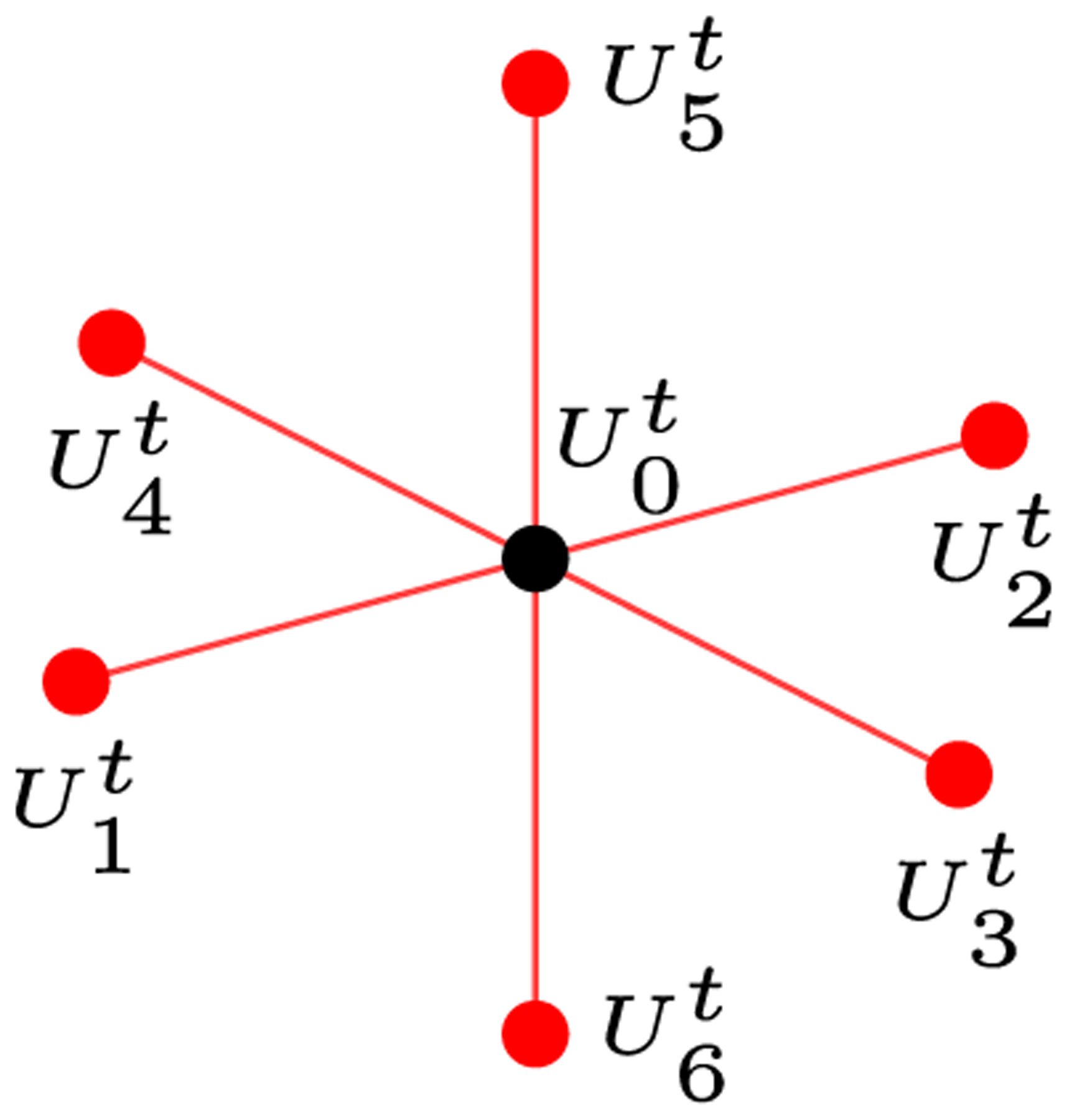
3D stencil representing data required for calculating the value at the next numerical time step t + 1 at each domain point U₀ using a standard second-order FDM

3.1 |. Sliding window strategy

The CUDA programming model requires mapping the problem to an array of thread blocks, called a grid. Figure 2 shows a simple mapping that can be used to assign threads to compute the numerical solution for mesh points. This thread structure also can help to hide memory access latency. The NVIDIA GPU hardware is designed to coalesce data into a single memory access to minimize the read latency from threads within a warp. In particular, single memory access to global memory returns 128 bytes in accordance with the GPU hardware architecture specification. This means that if all threads within a warp demand single precision floating-point values from 32 consecutive positions in global memory, when all required data can be retrieved with a single memory access. In this sense, by storing the 3D fields U and v with a linear data structure based on row-major order, it is possible to map threads into consecutive memory positions. This approach makes coalesced memory transactions to access data in the y and z directions possible, but x-direction accesses remain as not fully coalesced patterns. Figure 3 illustrates memory accesses that can be coalesced for y and z neighbors by using row-major order to store data. We can see, from left to right, memory positions accessed by consecutive warp threads when loading points (x, y, z − 1), (x, y − 1, z), (x, y, z), (x, y + 1, z), and (x, y, z + 1) in order to compute Equation (5). On the other hand, Figure 4 illustrates the x-direction memory access pattern. In the example of Figure 4, the eight threads represent a warp and every eight consecutive positions of global memory with different colors represent a different 128-byte word.

FIGURE 2.

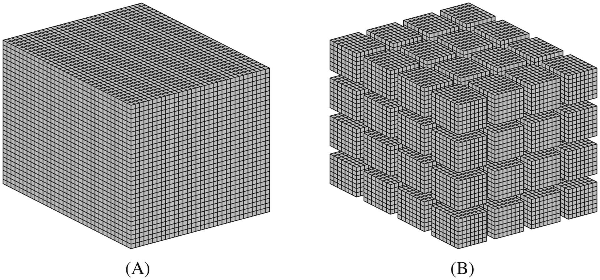
3D mesh used in FDM. A, non-partition domain; B, CUDA blocks partition

FIGURE 3.

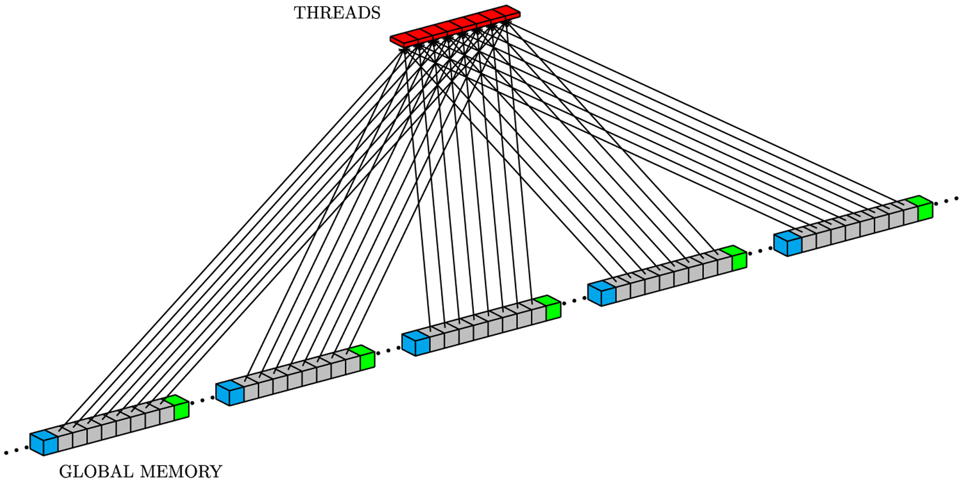
Representation of memory access pattern for sequential threads when computing Equation (5). From left to right, we show data required by each thread from points (x, y, z − 1), (x, y − 1, z), (x, y, z), (x, y + 1, z), and (x, y, z + 1)

FIGURE 4.

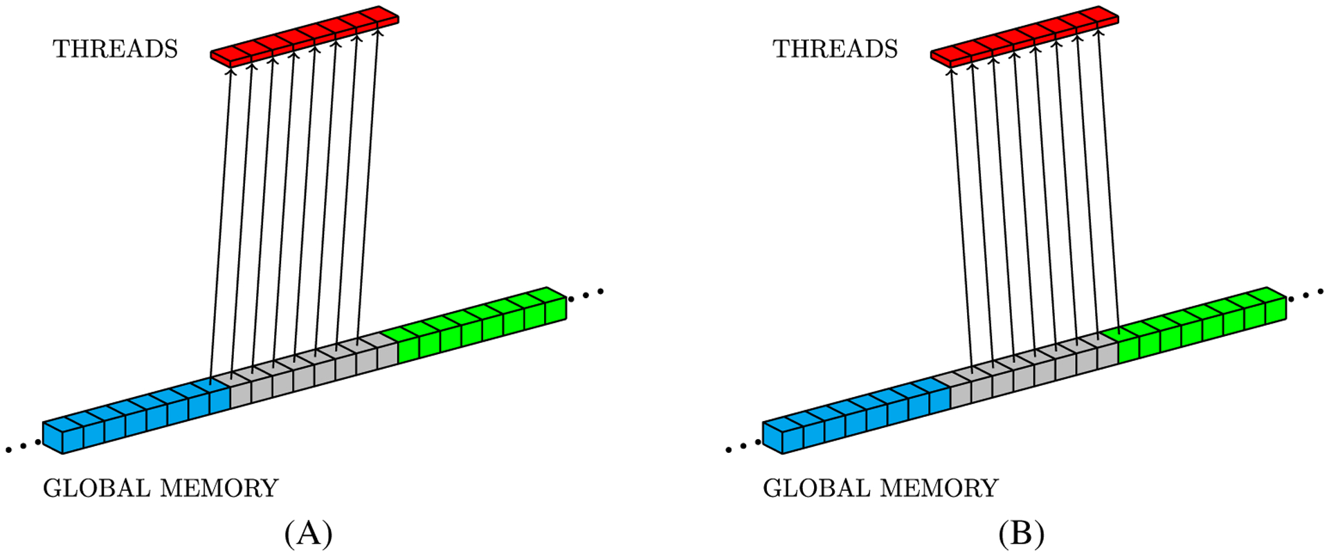
Representation of memory access pattern for sequential threads when accessing data from (x − 1, y, z) (a) and (x + 1, y, z) (b) to solve Equation (5). A, (x − 1, y, z) points; B, (x + 1, y, z) points

Global memory access pattern is an important performance consideration.⁶ Aligned access patterns like the ones in Figure 3 can be coalesced in single 128-byte memory transactions, while the ones in Figure 4 will need two 128-byte memory transactions. Carefully aligned data can improve a CUDA program by coalescing the maximum amount of data in a minimum number of global memory transactions.

Data organization using row-major order helps to reduce the memory access problem caused by requirements for data from neighbors and issues of spatial locality when solving the FDM discretization on a GPU. However, as each thread within a block will need its own data plus its six neighbors, this may lead to data access redundancy.^{7–9,11,19,21} This happens because, although using row-major order enables some coalesced memory accesses for block warps, all blocks in the grid will compete for space in the cache. This means that the chance of a cache miss increases as the grid size grows. For example, consider a thread k in the middle of a warp. According to Equation (5), at the time thread k asks for data in position (x + 1, y, z), thread k + 1 had requested this same data already, so it should be in cache memory. However, as several warps in different blocks are requesting data from global memory, there is a high probability that this data value will not remain in the cache anymore. Micikevicius proposed the sliding window approach to compute the 3D FDM stencil in Equation (5).¹⁹ The author’s approach uses a grid of 2D blocks that process the mesh through Z, using shared memory to store, for each z in the mesh, the cells to be processed and the XY neighborhood of the block. The block neighborhoods across Z are stored in the registers. According to the work of Micikevicius, the grid of 2D blocks saves GPU resources by block, enabling the concurrent execution of more blocks. He also demonstrates the reduction of memory access redundancies when storing data in shared memory before computing the stencil. This approach has been used by several authors through the years.^7–9,11,21

In CUDA, threads of the same block can communicate with each other through shared memory, which is a low-latency memory, but limited in total storage. For the numerical Laplacian solution on GPU, where each mesh point requires its current value and values at neighboring grid points (Figure 1), the sliding window strategy uses neighboring threads to load neighbor grid point values from global memory to shared memory. However, threads at the border of a block also copy data corresponding to the data of its neighbors which belong to a neighboring block, because GPUs cannot synchronize threads of different blocks. Figure 5 illustrates a block neighbor data. In this case, red, gray, and yellow cubes represent data that will be processed by a CUDA block, while other colored cubes (blue, orange, green, and light blue) represent data that will be processed by other CUDA blocks. The sliding window approach stores data from yellow and red neighborhoods in registers and data from all other cubes are stored in shared memory. Gray cubes represent data that will be operated on during the present iteration; at each new iteration, (1) data from the yellow neighborhood in registers will be replaced by the core data (gray cubes) from shared memory; (2) core data in shared memory will be replaced by the data from the red neighborhood in registers; and (3) data from the red neighborhood in registers will be replaced by new data from global memory. Figures 6 to 8 depict the access pattern to bring from global memory the data that will be stored in shared memory. In this example, our warp is represented by 8 consecutive threads (red squares) and the coalesced 128-byte data for eight consecutive global memory positions (gray cubes). Figures 6 and 7 exhibit coalesced access patterns, while the pattern of Figure 8 exhibits not only inefficient memory accesses but also divergence between threads in the same warp. The term inefficient is used here to address the fact that two threads per warp will access 4 bytes each, and for blocks with more than 30 threads in y-direction, this data will not be completely coalesced.

FIGURE 5.

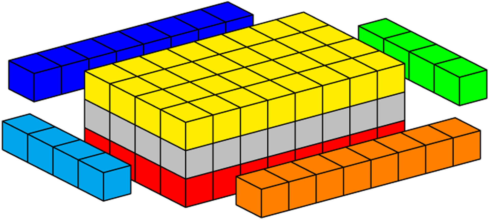
Geometric representation of data required by a 2D CUDA block. Colored cells highlight neighboring data required for computation

FIGURE 6.

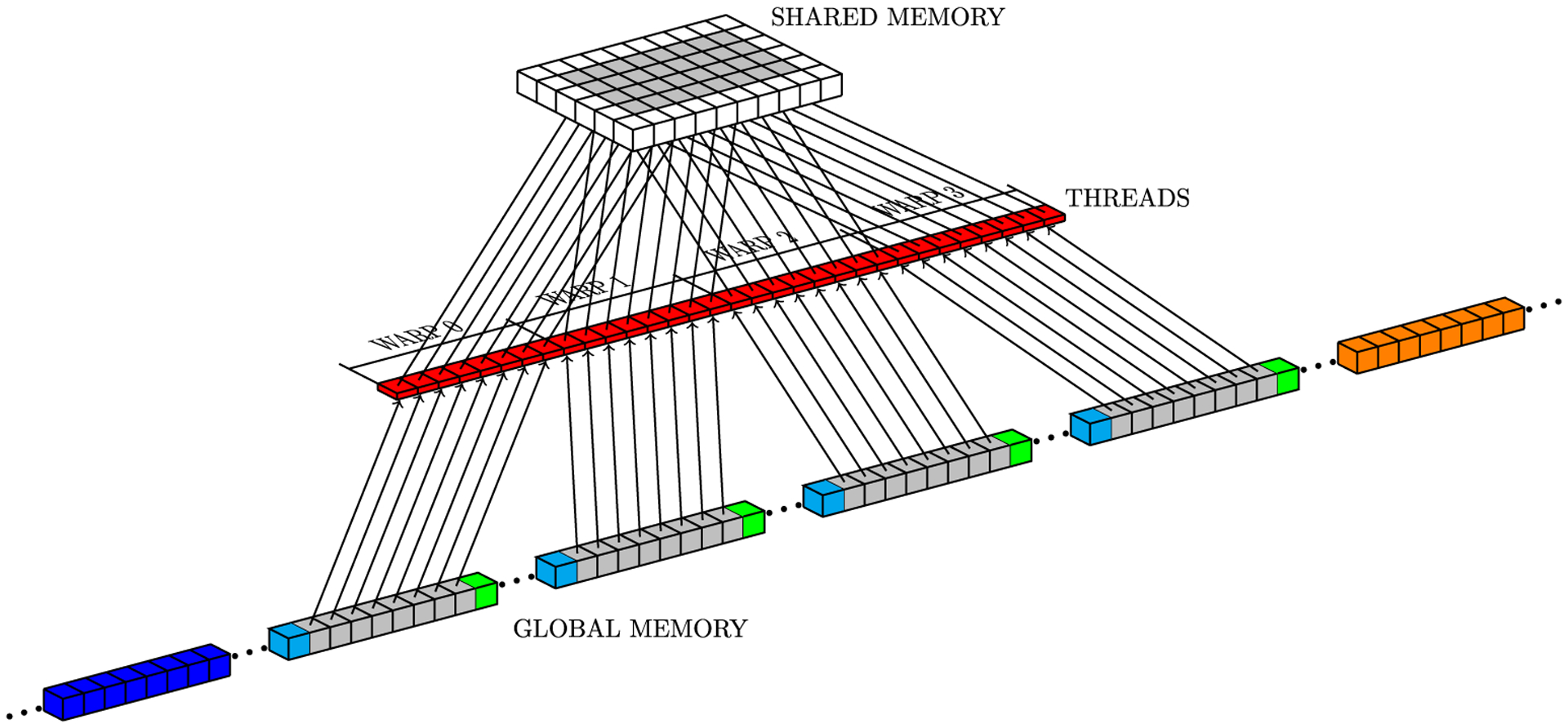
Access pattern for core data on global memory

FIGURE 8.

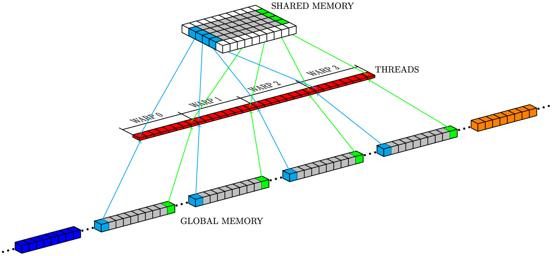
Access pattern for x neighborhoods

FIGURE 7.

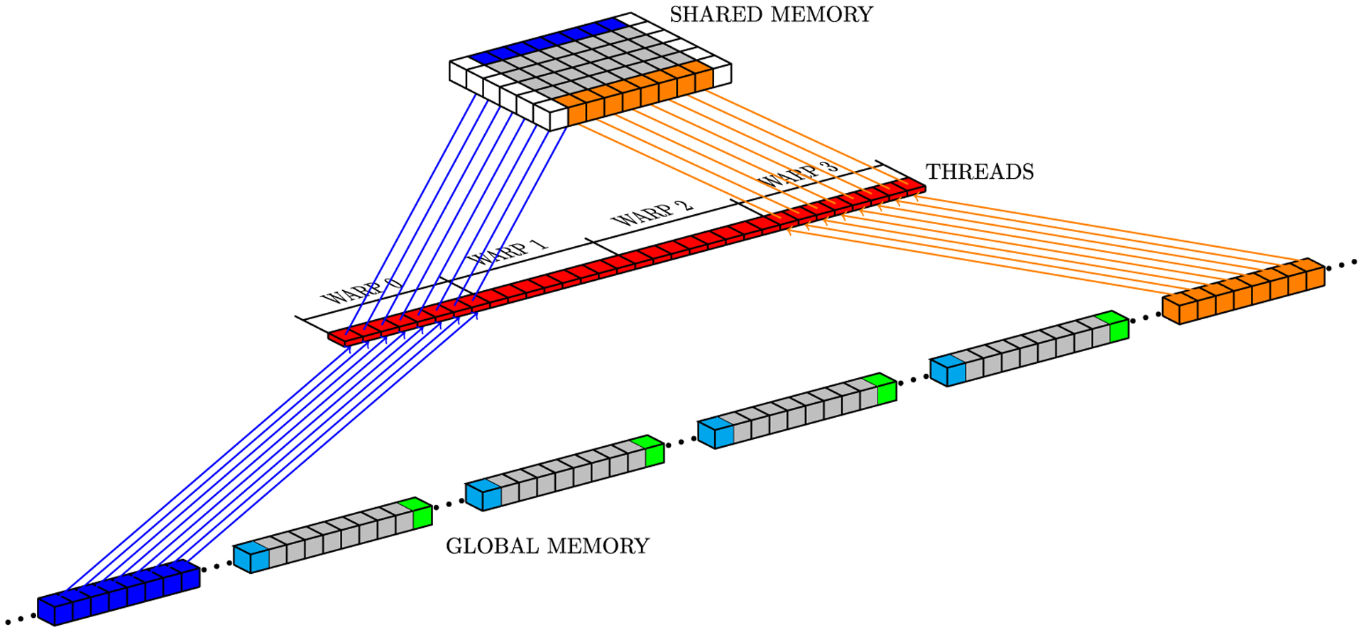
Access pattern for y neighborhoods

3.2 |. Coalescence optimization with a redesigned data structure

Two aspects of the straightforward approach compromise GPU performance, ie, (1) threads in the same warp that execute divergent code, which implies serialization within this stage and loss of massively parallel features; and (2) inefficient memory accesses (high number of memory transactions is required). Both problems usually occur in threads at the border of a thread block.

In order to minimize code divergence and maximize coalescence memory accesses in the classic sliding window solution, we propose a novel data structure to store the membrane potential U in the GPU global memory. Figure 9 depicts a representation of the general idea behind our proposal. In a row-major ordering, we store data for all domain points as a single memory buffer (Figure 2A). Our approach splits mesh points into smaller towers, so that it is possible to store data independently for each tower. Then, we also include one or more lines per tower (extra memory buffer); this new line stores replicated data from the light blue and green neighborhoods (Figure 9C) to maximize coalescence memory accesses and reduce code divergence when a block loads this data to its shared memory.

FIGURE 9.

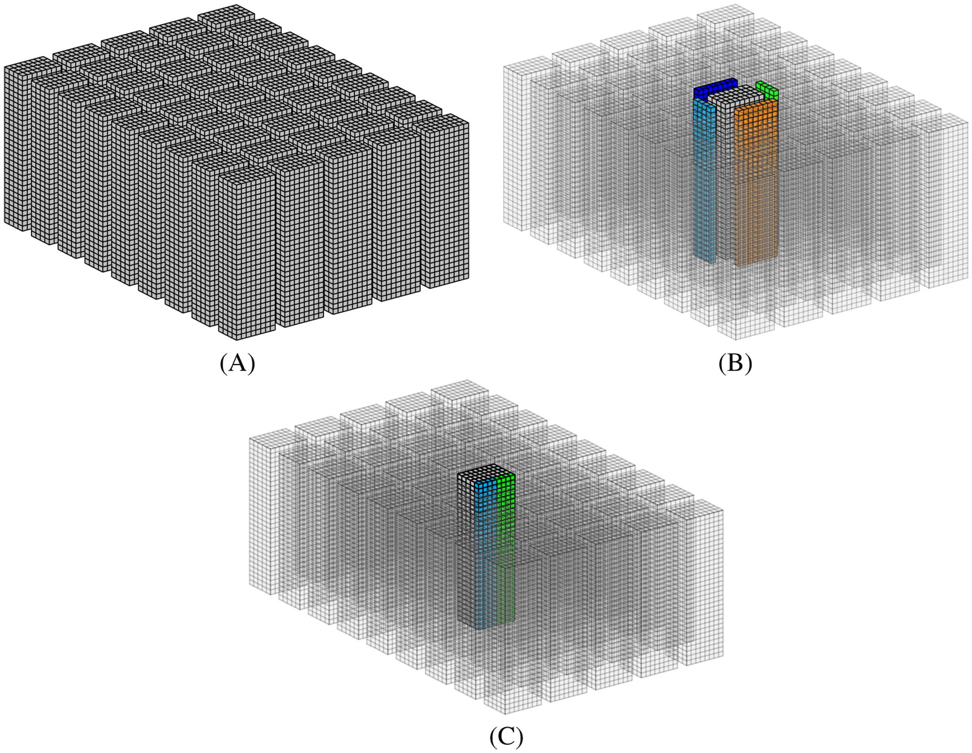
3D data structure representation for a 32 × 32 × 32 mesh. A, Mesh division in towers; B, Tower neighborhood; C, Proposed data structure

Figure 10 illustrates a 3D mesh data stored in memory linearly. Figure 10A shows a tile and its neighborhood, representing a z slice of a mesh tower (Figure 9A). Figure 10B shows how data are rearranged in the tower data structure. Finally, in Figure 10C, we can see how tile data (gray cubes) and the neighbors (colored cubes) actually are organized in the 1D array used to store it in global memory.

FIGURE 10.

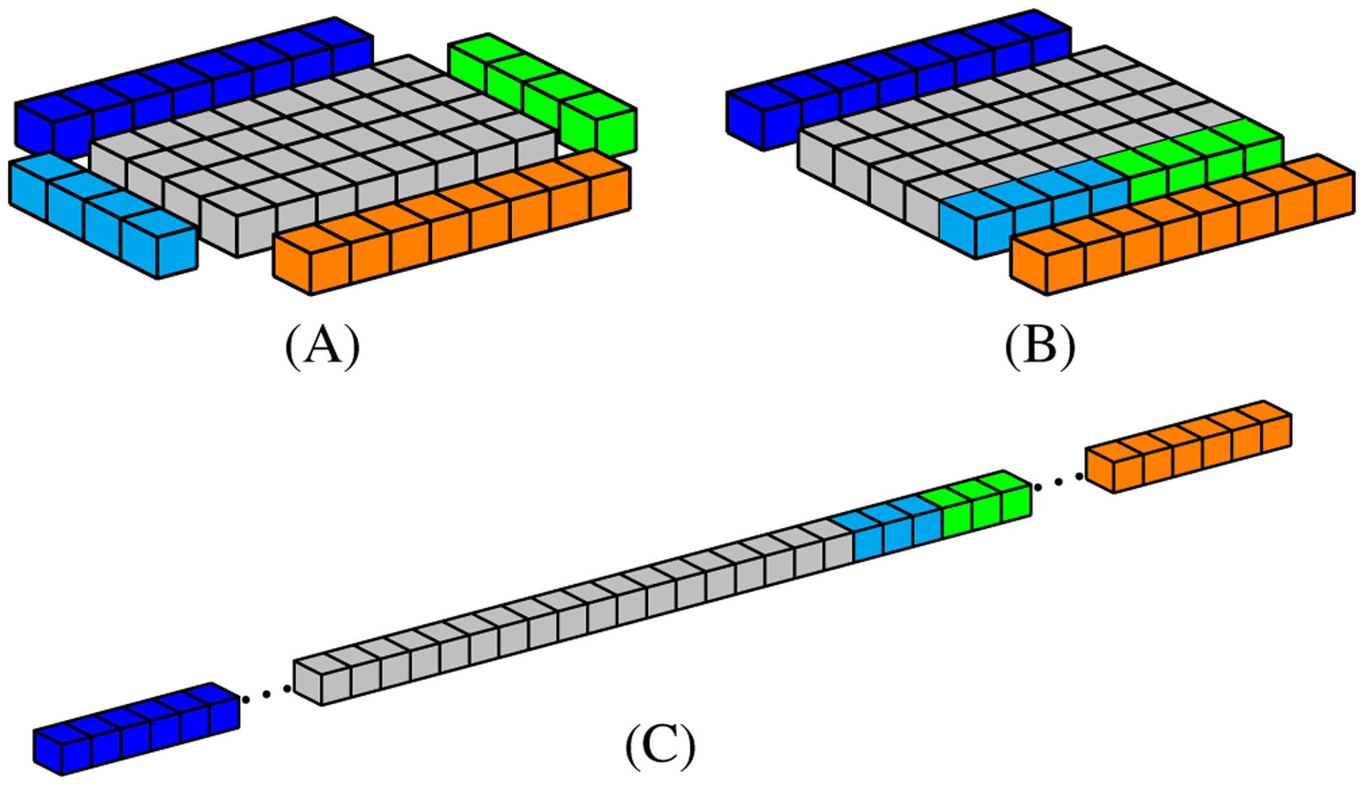
A simple representation of data positions to be accessed by a 8 × 4 thread block. A, Geometric data distribution in the mesh; B, Geometric data distribution in the proposed structure; C, Data distribution in global memory

Our proposed optimized strategy requires three steps, ie, (1) map threads into positions of the 1D data structure, (2) read data from global memory, and (3) write data to global memory.

Algorithm 1 illustrates the proposed data structure. The input variables are the following:

• thread index threadIdx;

• thread block index blockIdx;

• thread block size blockDim;

• grid size gridDim;

• mesh position z.

wlsize_x and wlsize_y represent the number of cells per tower, respectively, in the x and y directions (gray cubes in Figure 9C). wall_length is the number of cells in a single z slice of a tower (1D continuous structure formed by gray, light blue and green cubes in Figure 10C). Function WLCDSIDX returns an index that relies on the thread block index (blockIdx.x and blockIdx.y) and the size of the mesh in the z direction, establishing a correspondence between a thread block and a domain tower, and, consequently, between a thread and a position in the 1D data structure.

To avoid threads that will perform only memory accesses, our strategy proposes to launch a grid of threads that will fit the real mesh (Figure 9A), and not the data structure (Figure 9C). In this case, our proposed kernel was designed to reuse threads to access neighbor data.

Algorithm 2 shows how we calculate a numerical time step reading and writing data to and from global memory using the proposed data structure. Lines 1 to 3 set a relation between a thread and a position in the mesh. This relation is important because the dependent variable v is stored in global memory using row-major order, without any change in the mesh structure. Lines 5 and 6 set the thread position within a thread block. They will be used to map threads into positions in shared memory and in our proposed data structure. The relation between thread blocks, their threads, and the data structure are defined in Algorithm 1.

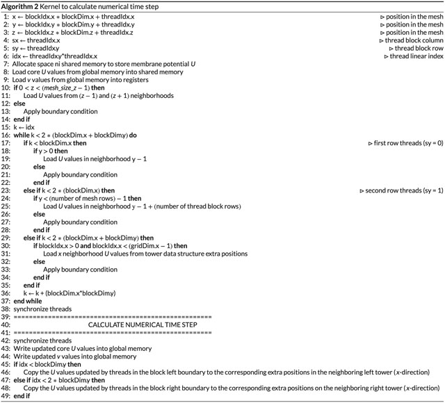
The tasks performed by Algorithm 2 consist of reading data from core memory positions (lines 8 and 9), reading data from the z neighborhoods (lines 10 to 14), reading data from the y neighborhoods (lines 17 to 28), reading data from the x neighborhoods (lines 29 to 35), synchronizing threads, computing new values for the dependent variables using the finite-difference approximation, synchronizing threads, and writing the new values to global memory (lines 43 to 49). As U values are stored in our proposed data structure, the block will use Algorithm 1 to locate data positions in global memory. As discussed in Section 3.1, threads will load U data from global to shared memory. The synchronization after loading the data to shared memory guarantees that, when the computation starts, all necessary data will be there for all threads. After the numerical time step computation, another synchronization is required to guarantee that all U values will be updated before writing them back to global memory.

Figure 11 shows a simple example of how Algorithm 2 accesses data in global memory. In this example, the tower has size 8 × 4 × 1. Red squares represent threads within the same block and arrows indicate the elements accessed by the threads. Figure 11A represents the execution of line 8 in Algorithm 2, while Figure 11B shows how memory positions hosting neighbor data are accessed in lines 17 through 35. The load tasks at lines 19, 15, and 31 are represented by blue, orange, and light blue and green arrows, respectively.

FIGURE 11.

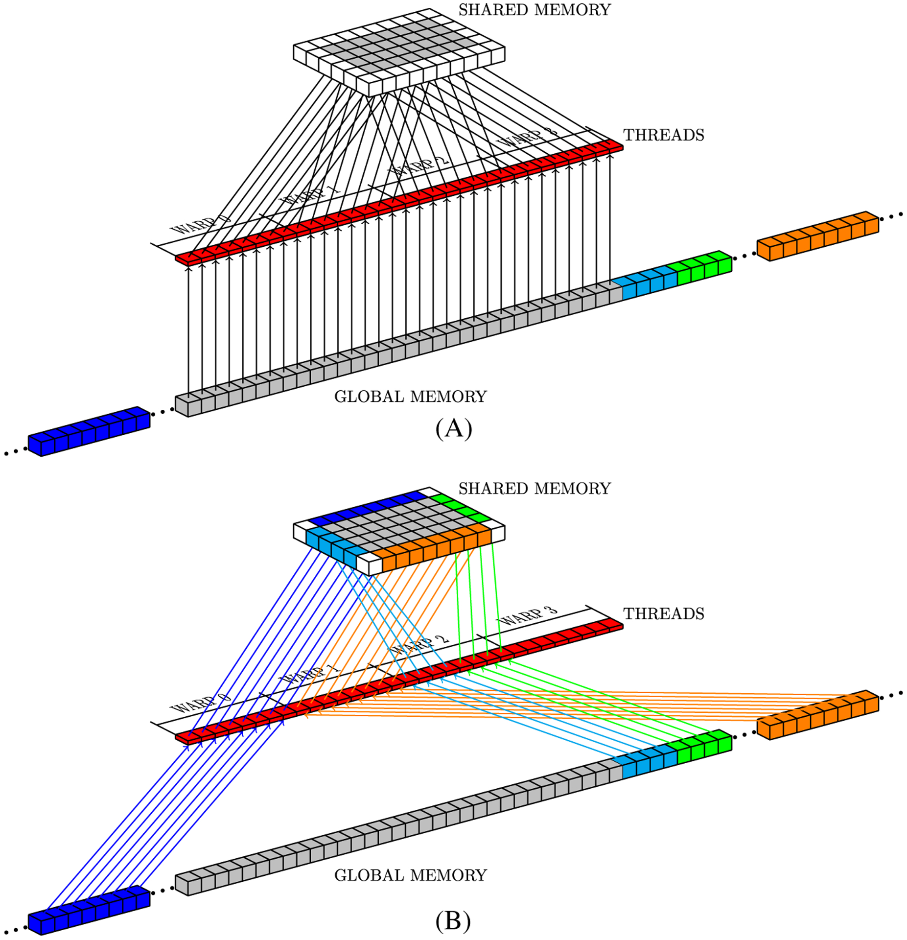
Global memory access pattern

The global memory writing task (lines 43 to 49 of Algorithm 2) is illustrated by Figure 12. In this figure, we use the geometric representation of the proposed data structure to facilitate showing the write pattern on neighboring towers. The tasks at lines 46 and 48 are represented by green and light blue arrows, respectively.

FIGURE 12.

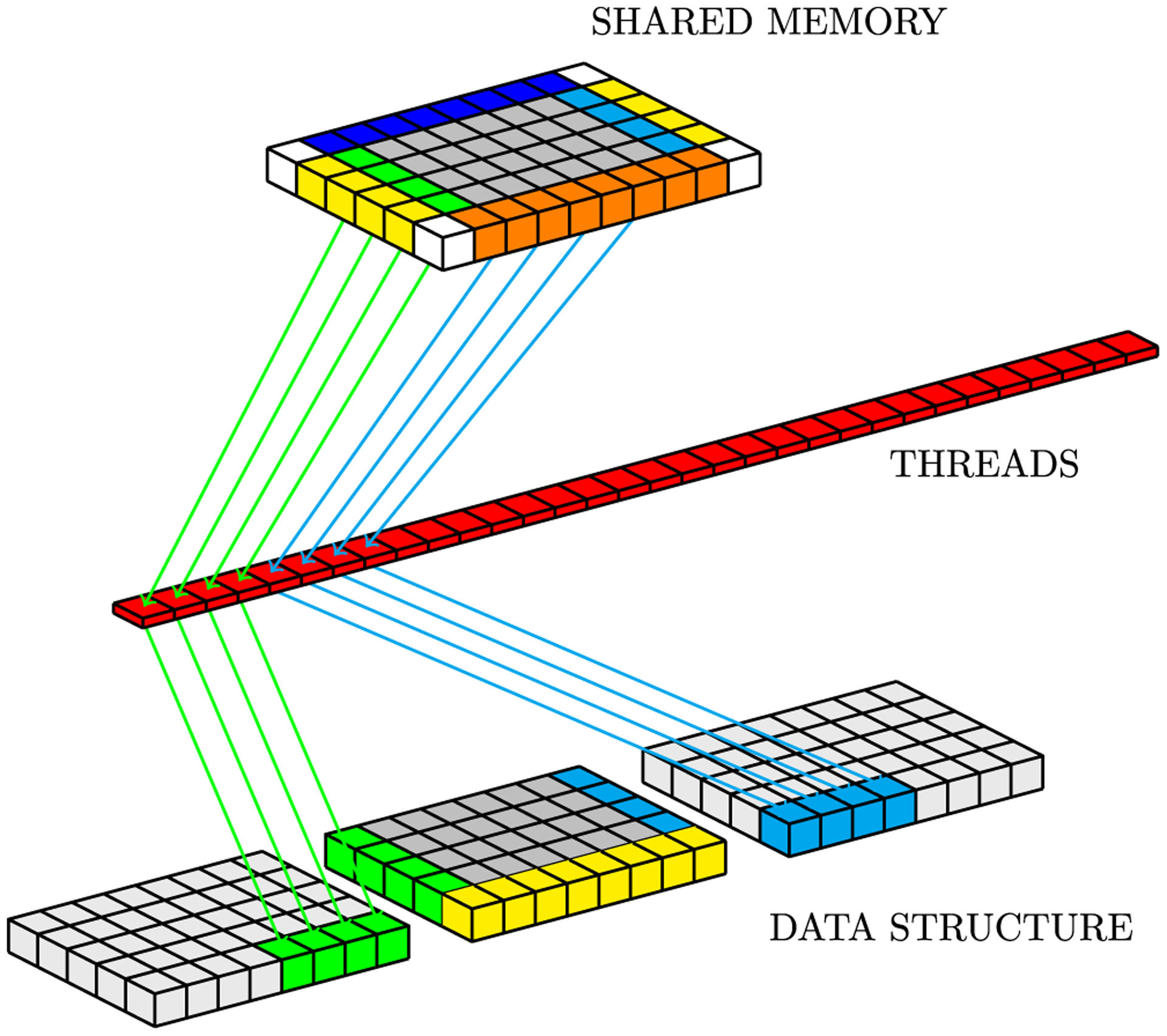
Global memory write pattern

4 |. RESULTS

In order to evaluate the proposed solution of the PDE (Equation (3)), we compare the classic sliding-window approach (Section 3.1) with our sliding window with the tower data structure. For convenience, hereafter we call the classic sliding window CSW and our proposed strategy as towerDS. We conducted experiments for three GPUs, namely, a GTX Titan X (Maxwell architecture), a GTX 1080 Ti (Pascal architecture), and a Tesla P100 (Pascal architecture), as a single-GPU test. We used an NVIDIA GPU cluster named DGX-1 (8 Tesla P100 GPUs) to execute the proposed approach in a multi-GPU environment. Table 1 summarizes characteristics of the CPUs and GPUs used in single-GPU experiments.

TABLE 1.

CPUs and GPUs characteristics

CPU	CPU cores	host RAM memory	GPU	GPU cores	GPU RAM memory
Intel Core i7-4790 (3.60 GHz)	4	32 GB	GeForce GTX Titan X	3072	12 GB
Intel Xeon E5-2620 (2.10 GHz)	8	32 GB	GeForce GTX 1080 Ti	3584	12 GB
2x Intel Xeon E5-2698 (2.2 GHz)	2x 20	512 GB	8x Tesla P100	8x 3584	8x 16 GB

Our implementations used CUDA version 9.0.176, the nvcc compiler, and nvprof as a profiler tool. Both machines were running Ubuntu 16.04. There were no memory copies between the CPU and GPU, and we adopted the same initial conditions for both implementations. All fields were directly initialized by a GPU kernel and stored in GPU global memory. Table 2 shows the amount of global memory demanded by each strategy. We calculate the theoretical memory space (in bytes) for single precision implementation as follows:

$$\mathit{\text{mem}}=4*(2*\mathit{\text{ds\_size}}+\mathit{\text{mesh\_size}}),$$ (6)

where ds_size is the number of cells in our tower data structure and mesh_size is the number of points in the mesh. ds_size is dependent on tower size and the number of towers required to represent the discrete domain mesh. In order to compute the amount of memory for CSW, we set ds_size = mesh_size. For example, to fit a discrete domain with 64³ cells, it will be required 2×8×1 towers with 32×8×64 cells each, resulting in ds_size = 278528 cells.

TABLE 2.

GPU global memory space required to store all necessary fields for a simulation. Memory space is presented in Mb

mesh_size	ds_size	CSW	towerDS
2563	17 825 792	192.00	200.00
5123	142 606 336	1536.00	1600.00

4.1 |. Numerical experiments

In both approaches (CSW and towerDS), the computation of one time step consists of one invocation of the kernel that solves Equation (5). We designed a set of experiments to executed simulation with varying mesh and block sizes. In addition, to guarantee the data consistency of the simulations, we compared a pulse propagation simulated with CSW and towerDS based on the same initial condition.

We conducted the experiments using a time step of 0.05 ms. The spatial resolution was equal in all axes (Δx = Δy = Δz) and depended on the domain mesh size. The initial condition was given by

$$U_{ijk}^0=3.0\hspace{1em}\text{ for }{z}_k\le 0.05*(\mathit{\text{mesh size }}z)$$ (7)

$$v_{ijk}^0=0.5\hspace{1em}\text{ for all }{z}_k.$$ (8)

In our experiments, we simulated a total of one second (1s); therefore, the time domain discretization generates 20 000 time steps.

4.2 |. Single GPU performance evaluation

To evaluate how the block size affects computation time, we fixed the mesh size and varied the block size. The elapsed time was measured with cudaEvents. Figures 13 to 15 show our experimental results for three different GPUs, the GTX 1080Ti, GTX Titan X, and Tesla P100, respectively. In all these three figures, the upper plots exhibit how GPU elapsed time behaves as the block size was changed, while the bottom plots shows times relative to the fastest configuration for that experiment. Our results show that increasing the block size over X causes a significant reduction in the overall GPU processing time. As accessing data in halos between blocks over X is our major source of memory accesses issues and code divergence (see Section 3.1), this behavior is expected.²²

FIGURE 13.

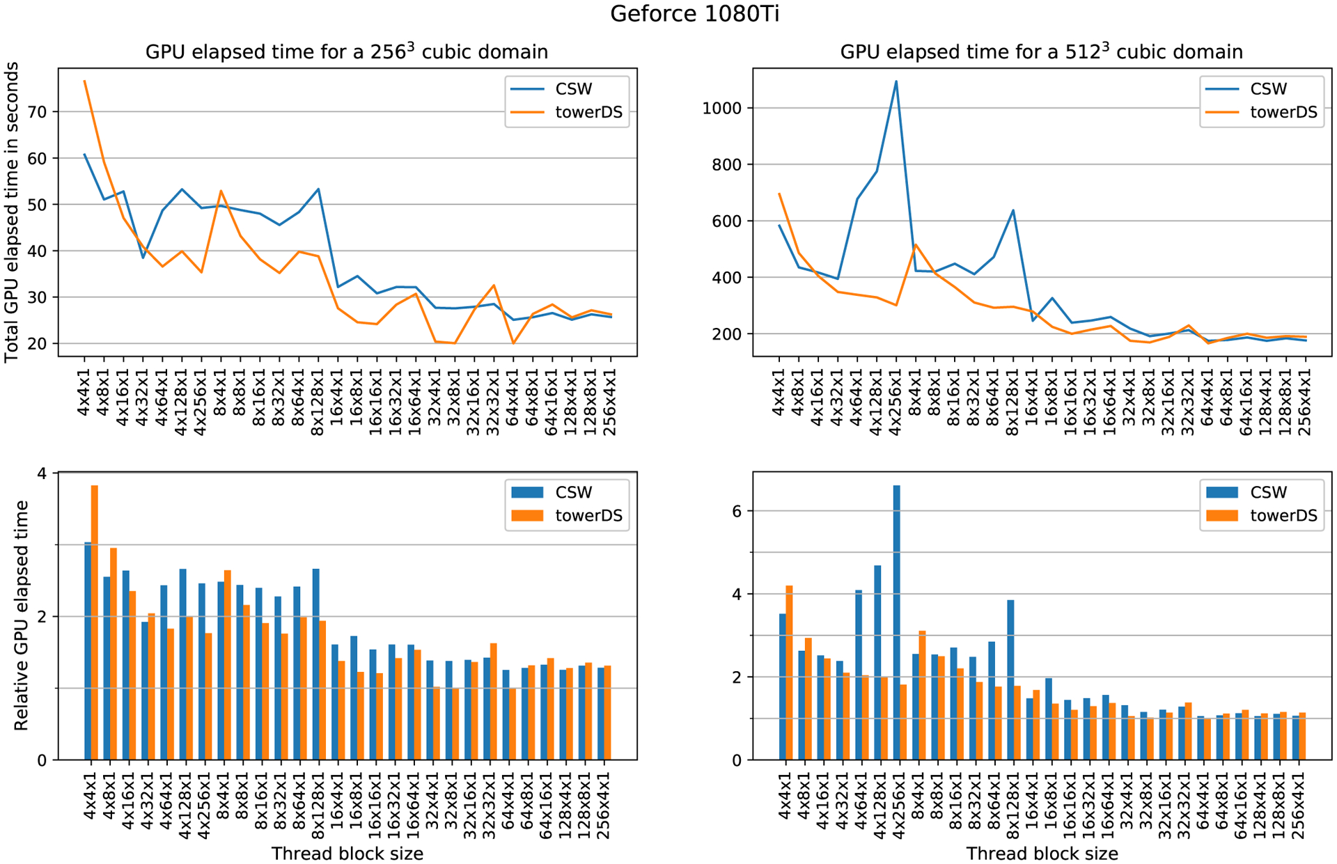
Computation time as function of block size for GTX 1080 Ti. This experiment computed 20 000 time steps

FIGURE 15.

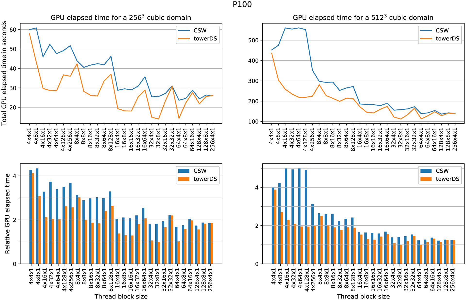
Computation time as function of block size for Tesla P100. This experiment computed 20 000 time steps

Table 3 presents the block and thread arrangements that achieved the best performance with both approaches, ie, towerDS and CSW. In general, the smallest execution times were achieved with 64 × 4 × 1 blocks. The exceptions happened for the Tesla P100, in which the best arrangement depends on the mesh size and the approach adopted.

TABLE 3.

Fastest block configurations to compute 20 000 time steps

Mesh size	GPU	CSW		towerDS
		time	block size	time	block size
256	1080Ti	25.0849	64 × 4 × 1	20.0084	64 × 4 × 1
	Titan X	33.7281	64 × 4 × 1	34.8525	64 × 4 × 1
	P100	23.6460	64 × 4 × 1	14.0196	32 × 8 × 1
512	1080Ti	174.3350	64 × 4 × 1	165.5145	64 × 4 × 1
	Titan X	255.8197	64 × 4 × 1	238.4309	64 × 4 × 1
	P100	136.3548	128 × 4 × 1	112.2918	32 × 8 × 1

The time reduction we achieve with our proposed towerDS approached 40.71% for a 256³ mesh using the Tesla P100. For the 512³, we could reduce the execution time by 17.65% also using the Tesla P100. For the GTX GPUs, the Titan X performs better for the 512³ mesh (time reduction of 6.8%), while the 1080Ti performs better for the 256³ mesh (time reduction of 20.24%).

4.3 |. Multi-GPU experiments

During our experiments, we observed that GPU global memory space could be an issue. Equation (6) depicts the amount of memory space required by a simulation. For a mesh with 1024 × 1024 × 1024 cells, eg, around 12.5 GB of memory space is required. In order to remove this constraint, we extended our solution to a multi-GPU environment.

Multi-GPU clusters use a distributed memory, ie, each GPU has its own memory. Thus, to execute our simulation (the cardiac electrical dynamics simulations) on a multi-GPU cluster, it is necessary to split the domain into sub-domains, so that each GPU can compute part of the problem. As each GPU is responsible for computing a sub-domain and a Laplace discretization (Equation (5)) requires information from neighbor cells, each GPU must communicate with other GPUs in order to send and receive information of neighboring cells that are computed in different GPUs. We choose to split our domain in the z-direction, due the symmetry of the proposed data structure at this axis. Each sub-domain has two extra memory areas to store U data for the sub-domain z top and bottom boundaries. Figure 16 illustrates which data are stored in each extra memory area (communication buffers).

FIGURE 16.

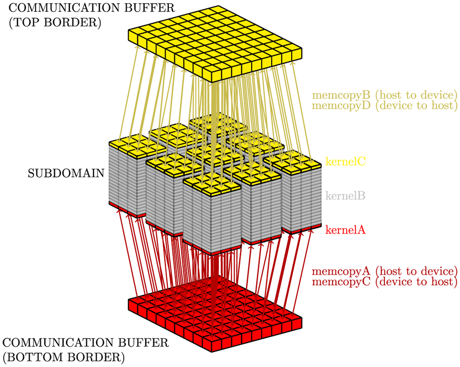
Sub-domain buffers used to communicate z borders between different GPUs. The right side of the figure shows the scheme used with the multi-GPU/multi-stream strategy

For each time step, each GPU copies its z boundaries to the CPU RAM memory. Then, each CPU copies the data for the respective neighbor sub-domains on other GPUs. As an example, consider the kth sub-domain, assigned to GPU number k. On time step n, GPU k copies to CPU RAM memory the top and bottom z-boundaries of sub-domain k. Before the computation of time step n + 1 begins, the CPU copies the top z-boundary of sub-domain k to the bottom extra z slice of GPU k + 1, and the bottom z-boundary of sub-domain k to the top extra z slice of GPU k − 1. Figure 17 illustrates the communication pattern we designed. Gray rectangles represent sub-domains, colored bars inside sub-domains represent their z-boundaries, colored bars outside sub-domains represents their z-neighborhoods, and colored arrows represent memory copies.

FIGURE 17.

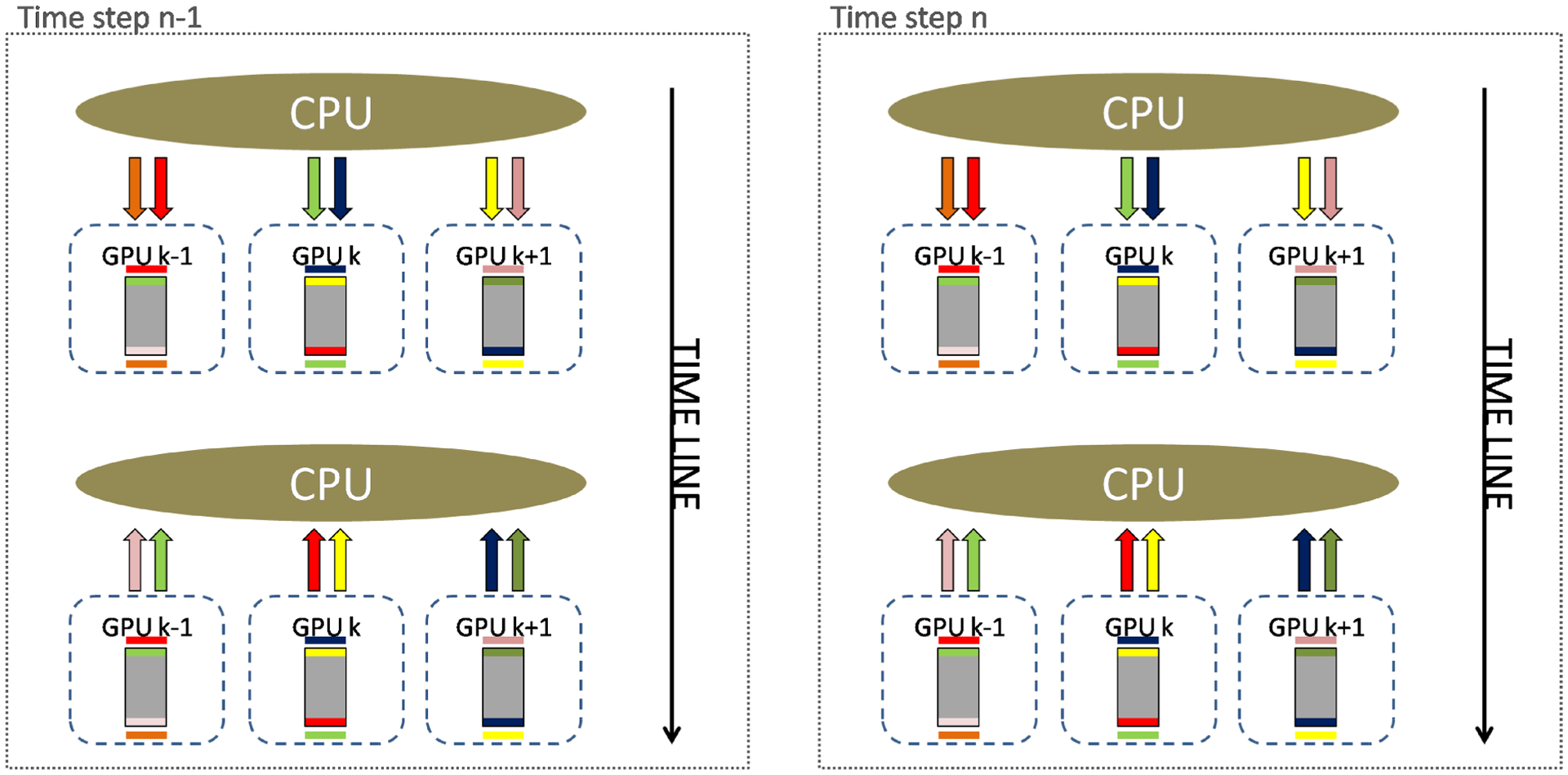
Communication strategy for three sequential GPUs during the computation of two consecutive time steps

Our multi-GPU experiments were performed on an NVIDIA DGX-1. This GPU cluster is composed of eight NVIDIA Tesla P100 GPUs, each with 3584 CUDA cores. The achieved results with a direct implementation of our multi-GPU approach show that, when we increase the number of GPUs, the overall time also increases (blue and red lines in Figure 18). This problem occurs due to the growth of memory transactions.

FIGURE 18.

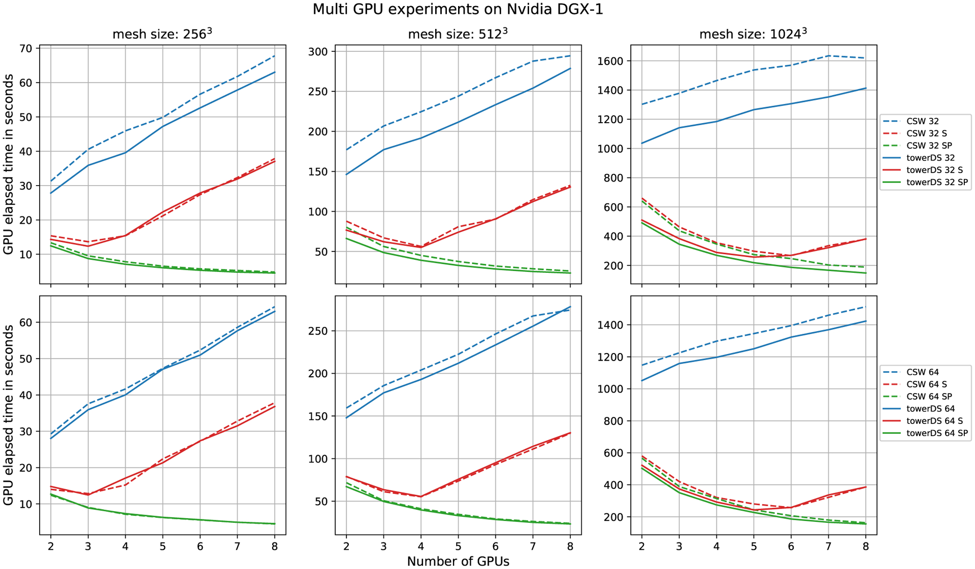
Performance evaluation of different multi-GPU strategies. The letter S in the legends means streams strategy and SP means stream + page-lock memory

Concurrency between processing and memory copies can be applied to reduce the memory copy latency.²³ In our single approach, on each time step computation, we copy memory from the CPU to the GPU (communication buffers), run a single kernel to solve Equation (5), and then copy memory from the GPU to the CPU (communication buffers), ie, computation and communication are executed in batch, limiting the performance by copy memory between CPU and GPU, which represents the slowest step.

With this in mind, we proposed the use of two streams. The first computes Equation (5), as long as the second is responsible for communication. This approach tries to overlap the steps and minimize the simulation time. Thus, this approach consists of three kernels, ie, the first processes the sub-domain bottom boundary (kernelA), the second processes the sub-domain top boundary (kernelC), and the third process all other z-layers (kernelB), as illustrated in Figure 16. Furthermore, the memory copy step is composed of four memory copy tasks, ie, tasks memcopyA and memcopyC copy the bottom communication buffer from CPU to GPU (memcopyA) and from GPU to CPU (memcopyC); tasks memcopyB and memcopyD copy the top communication buffer from CPU to GPU (memcopyB) and from GPU to CPU (memcopyD).

Figure 18 presents the results achieved with the stream approach and the scalability of multi-GPUs, considering 20 000 numerical time steps and three domains, ie, 256³, 512³, and 1024³. We evaluate the behavior of three approaches using our memory copy strategy, ie, one standard with only a single stream, one using our three-stream strategy to overlap computation and memory copy (identified by letter S in Figure 18), and one using our three-stream strategy plus page-lock or pinned host memory (identified by letters SP in Figure 18). Our approach used page-lock or pinned host memory in order to guarantee the overlapping memory copy. This flag on the host allocation was set with the API cudaHostAlloc().

Page-lock or pinned host memory enables faster memory copies between the CPU and GPU²³ by guaranteeing that the memory is not swapped in secondary memory, ie, data in page-locked memory is available to copy any time, avoiding time wasted with loading data from secondary memory.

The multi-GPU scalability is sub-linear in the page-locked memory approach (Figure 18). Indeed, eight GPUs obtain a performance gain slightly higher than seven, for instance. On the order hand, four GPUs presented a performance almost four times faster than one. Thus, four GPUs obtained the best performance considering scalability. However, more GPUs may be necessary for the domain size using distributed memory. The multi-GPU scalability is related to the amount of data processed by each core versus the amount of data communication. With this in mind, Figure 18 shows that more than four GPUs increases the amount of data copied. However, the amount of data computed by each core is constant (Equation (5)). Thus, the communication time turns to be dominant in the total simulation time. On the other hand, when using two to four GPUs, the computation time is dominant and presents scalability that is close to linear. Table 4 shows the faster results achieved with eight GPUs, using CUDA streams and page-lock memory.

TABLE 4.

GPU elapsed time to run 20 000 time steps

Mesh size	CSW		towerDS
	time	block size	time	block size
2563	4.4975	64 × 4 × 1	4.5418	32 × 8 × 1
5123	24.0151	64 × 4 × 1	23.0818	32 × 8 × 1
10243	162.9126	64 × 4 × 1	147.9537	32 × 8 × 1

Figure 19 shows the number of cells processed per second for all different GPUs we have tested. We chose the fastest block configuration for each case. We achieved the same number of grid points processed per second for both mesh sizes, ie, 256³ and 512³. As this result was achieved with the same block sizes, we reached full occupancy of the GPU in both cases. On the other hand, our multi-GPU approach performs better for bigger meshes and is most efficient for the 1024³ mesh. Table 5 shows the number of time steps computed per second for our fastest single- and multi-GPU experiments.

FIGURE 19.

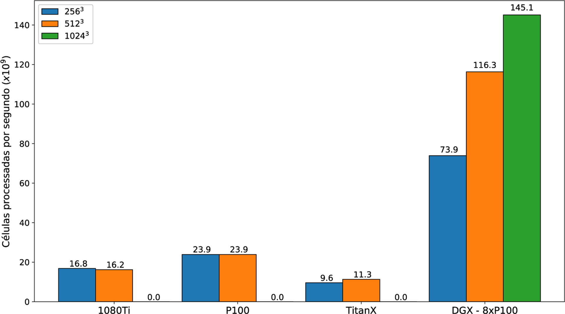
Average number of cells processed per second for the fastest block setup for each experiment

TABLE 5.

Time steps computed per second for our faster single- and multi-GPU experiments

GPU	2563	5123	10243
P100	1426	178	–
DGX - 8xP100	4405	866	135

4.4 |. Coherence between simulation outputs

Figure 20 illustrates qualitative results of the proposed novel memory-access model for optimizing simulations of cardiac electrical dynamics. We compared output potential fields for simulations with both discussed strategies. We saved fields in 2000 different time stamps and simulated 1 second of physical time. We verified that the data are consistent and there is no difference between them.

FIGURE 20.

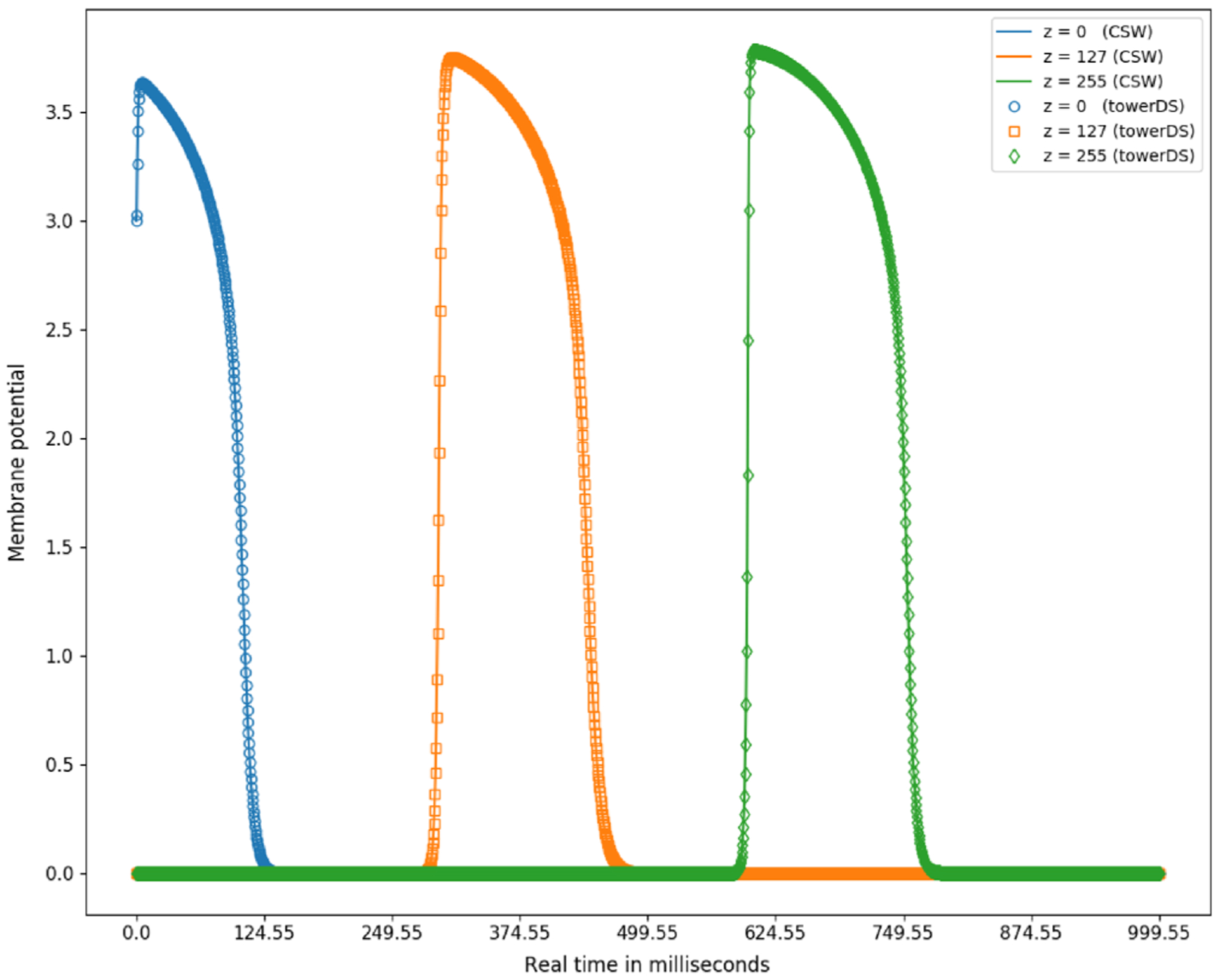
Electrical stimulus propagation along the z direction

Figure 21 depicts the pulse propagation in a 3D cubic mesh with side 256 and computed using the towerDS strategy. The space between frames is 25 milliseconds and we initiate a spiral wave by introducing a stimulus of the form

$${\cup }_{x,y,z}^{8,500}=\{\begin{array}{ll}3.0f\hfill & \text{ if }60<z<100\text{ and }117\le x\le 137\hfill \\ {\cup }_{x,y,z}^{8,500}\hfill & \text{otherwise}.\hfill \end{array}$$ (9)

FIGURE 21.

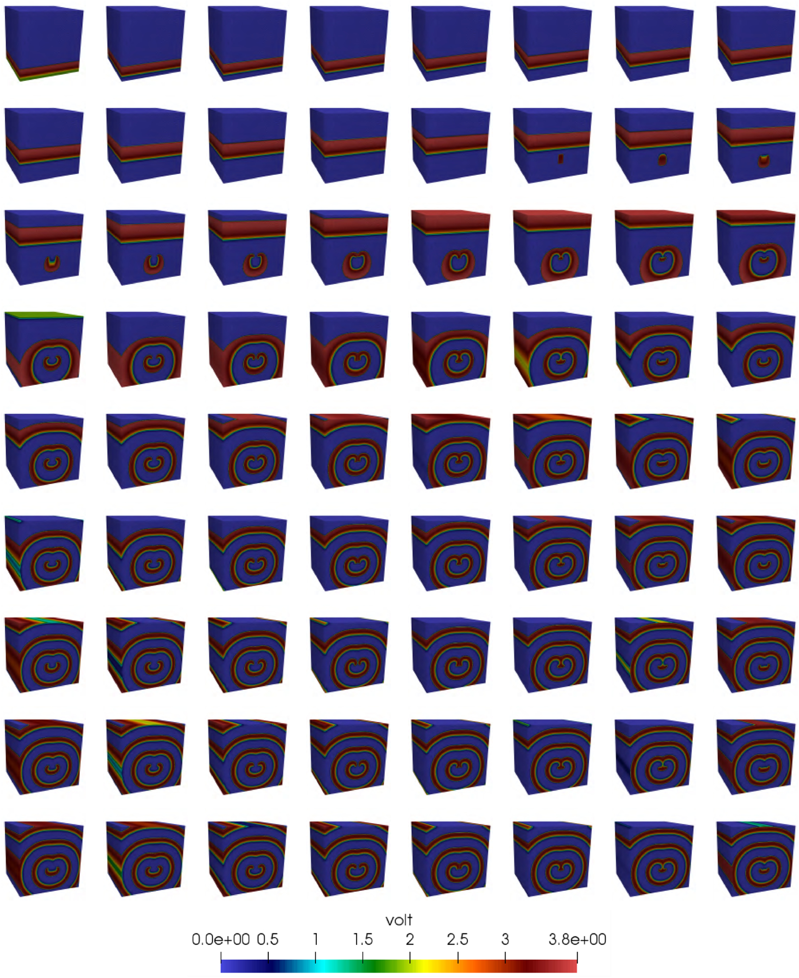
Spiral wave simulated with our towerDS implementation for 2 seconds of physical time (40 000 time steps)

The initial and boundary conditions are the same used in all our experiments. Initial conditions are described by Equations (7) and (8). For boundaries, we enforce no-flux boundary conditions by mirroring data from the internal neighbors. Figure 22 depicts the boundary conditions for a simple 8 × 8 2D mesh.

FIGURE 22.

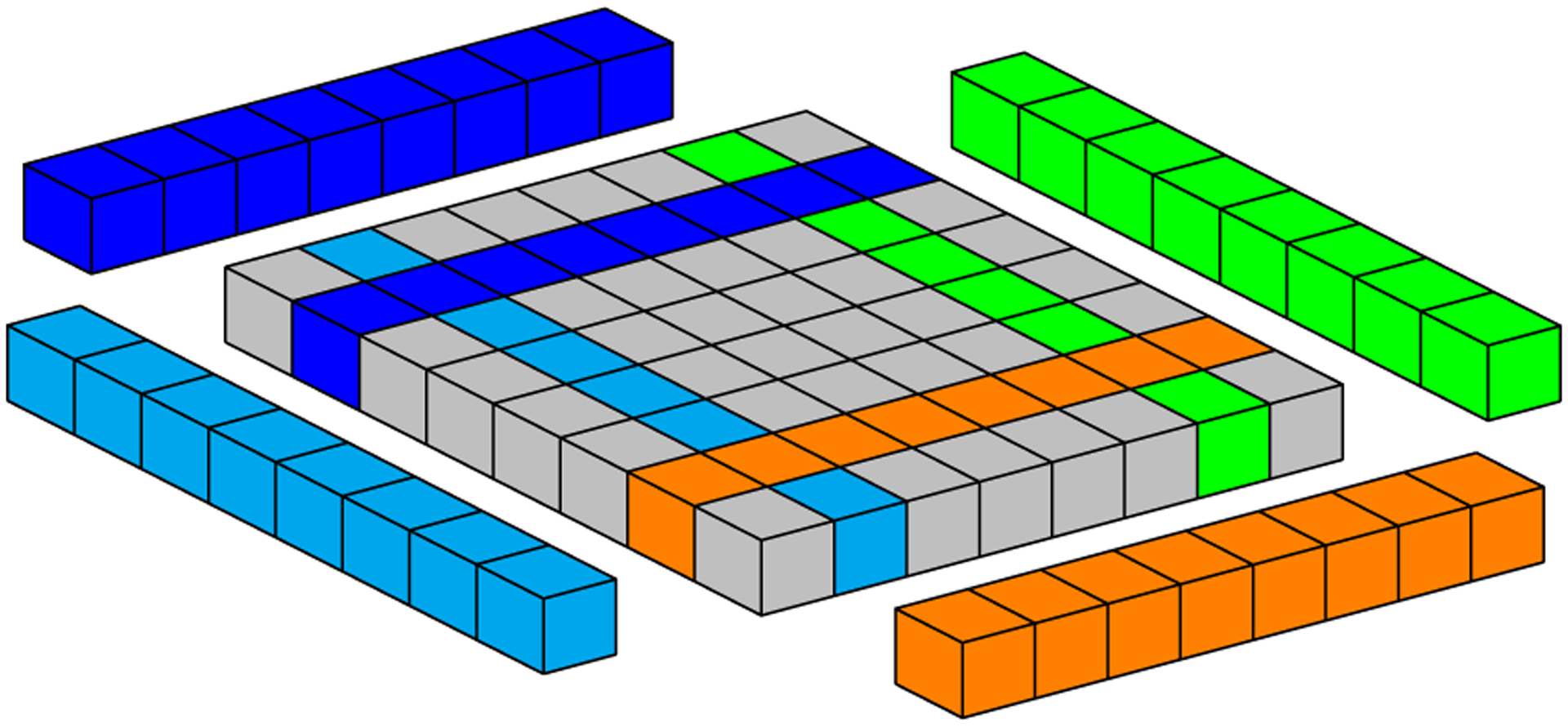
Mirror scheme applied as boundary conditions at mesh borders

5 |. RELATED WORK

Much effort has been devoted to accelerating computer simulations of cardiac electrophysiology towards real time, many of them requiring high-performance supercomputers.^24–27 However, supercomputers are expensive and have high maintenance requirements, and they may not be readily available to a broad group of users. For this reason, many researchers are turning to GPUs.

Over the last decade, GPU computational power increased in such a way that they may be used in place of supercomputers for specific scientific computational problems.^28,29 Cardiac electrical dynamics simulations is no exception to this trend.^30–32

Several authors have tested GPU performance previously for different cardiac tissue models. They evaluated not only the performance of adapted CPU implementations for GPUs,^33–35 but also different parallel strategies^{11,20,36–39} and numerical methods.^40,41

Some authors have addressed the problem of implementing a solution for a PDE like Equation (3) using FDM.^7,11,21 Bartocci et al¹¹ evaluated GPU implementations for cardiac tissue models with different complexities. They tried two different strategies to accelerate the PDE solution through memory optimization, ie, one using shared memory and the other using texture memory. Unlike our approach, they launched blocks with extra threads exclusively to read neighboring block data from global memory. Running on a Tesla C2070, their simulation with a 2D mesh composed of 2²² cells took almost 10 seconds using texture memory and just over 15 seconds using shared memory. With a similar but 3D mesh using 2²⁴ cells (4× more cells), we spent 20.68s. Although we use a better GPU than the work of Bartocci et al,¹¹ our 3D mesh requires more data accesses then their 2D mesh. Michéa and Komatitsch⁷ and Giles et al²¹ discussed GPU implementations for the wave equation and did not offer solutions for memory displacement in global memory accesses by threads on CUDA block borders.

Nimmagadda et al²⁰ explored a linear data structure in GPU simulations using a 2D bidomain model of cardiac electrophysiology. The authors ordered their data to enable WARP coalesced memory access, but they did not discuss the CUDA block border problem. They reported an acceleration of around 1.15 by changing the data ordering. Using a Tesla C1060, they reported a computation time around 1686 seconds to calculate 10 000 time steps in a 256 × 256 × 256 3D mesh. They remarked that 62% of this time (around 1045.6 seconds) was spent with the PDE solution. The authors also tried a multi-GPU approach and reported an acceleration for the PDE solution of around 14× compared with their single-GPU approach.

Xia et al³⁷ used linear structures to accelerate memory access when solving the diffusion term of Equation (1). The authors’ simulations performed 120 000 time steps in a 317 × 204 × 109 mesh, but only approximately 1 million are valid cell nodes (they omitted empty cells to avoid GPU performance degradation). Their optimization achieved better results using blocks with 64 threads. In this case, they reported a computation time a little over 500 seconds to calculate the solution using FDM and double-precision variables (this 500 seconds time took into account only the PDE solution). Our simulations have six times fewer time steps, but we processed 134 times more cells (512³) in just 112.30 seconds.

Some authors have tried different approaches or numerical methods for GPU implementations. Amorim and dos Santos⁴² proposed a GPU solver for a 2D bidomain model using the preconditioned conjugate gradient method⁴³ to solve the PDE. The authors reported a total simulation time of 18.3 seconds for a 513 × 1025 mesh. Mena et al³⁸ proposed a CUDA program combining the processing power of the GPU and CPU to accelerate explicit and semi-implicit methods to solve the reaction-diffusion equation. They reported speedups between 50 and 70 times for 3D meshes. Campos et al⁴¹ evaluated the application of Lattice Boltzmann method⁴⁴ to cardiac electrophysiology simulations. Using 256 threads per CUDA block, they reported overall computation times of 97 seconds for a 128³ mesh and 519 seconds for a 224³ mesh. These results were achieved for the eight-variable Luo-Rudy I model.⁴⁵

More recently, Kaboudian et al⁴⁶ proposed a WebGL-based approach to perform cardiac electrophysiology simulations on GPUs, using FDM and single precision. The authors compared spiral waves simulated with their WebGL approach with spiral waves from experimental data. For a simulation with a 3-variable model in a 2D domain with 512² points, they reported that is possible to run up to 38 000 time steps per second in a Titan X with Pascal architecture. This means they can process up to 9.96 × 10¹⁰ domain points (cells) per second. While their work present a good real time visualization result, they are constrained to small domains.

6 |. CONCLUSIONS AND FUTURE WORK

In this work, we have proposed a novel strategy to store and read data from GPU global memory. This strategy improved the computation of numerical solutions of the Laplace operator using a finite-difference discretization. We evaluated the strategy using a reaction-diffusion equation that models cardiac electrophysiology. The performance of our strategy changed with thread block size, but our proposed strategy accelerated almost all tested domain sizes and block sizes. The best single-GPU performance was attained for a 256³ mesh using 32 × 8 × 1 blocks, with a speedup of 1.4.

We also implemented a multi-GPU version of our proposed strategy. This multi-GPU version enabled us to run simulations with domains that a single GPU’s memory cannot support. We found that the performance of the multi-GPU simulations suffers from CPU-GPU memory copies, so we developed strategies based on memory copy/computation concurrency with CUDA streams to improve the performance of our multi-GPU implementation. We can also solve a domain with 256³ cells only 4 times slower than real time.

The proposed data structure is consistent with different GPU architectures, since we achieved similar results with three different GPUs, namely, the Titan X (older architecture), the 1080Ti, and the P100 (fastest GPU). In fact, the proposed data structure reduces memory data transfer, avoids clock cycle waste, and improves the GPU memory.

Our data structure was designed to store single-precision variables to enable coalesced memory transactions when accessing neighbor data for threads at block borders. We believe we could adapt it to double-precision variables, but this is a new aspect we will investigate in the future.

The proposed strategy offers a novel data structure, a data access algorithm, and a carefully planned thread block structure to provide a reliable and fast solution for the Laplace operator using a finite-difference discretization. We believe that the proposed strategy can help in the pursuit of real-time simulations of whole-heart models.

FIGURE 14.

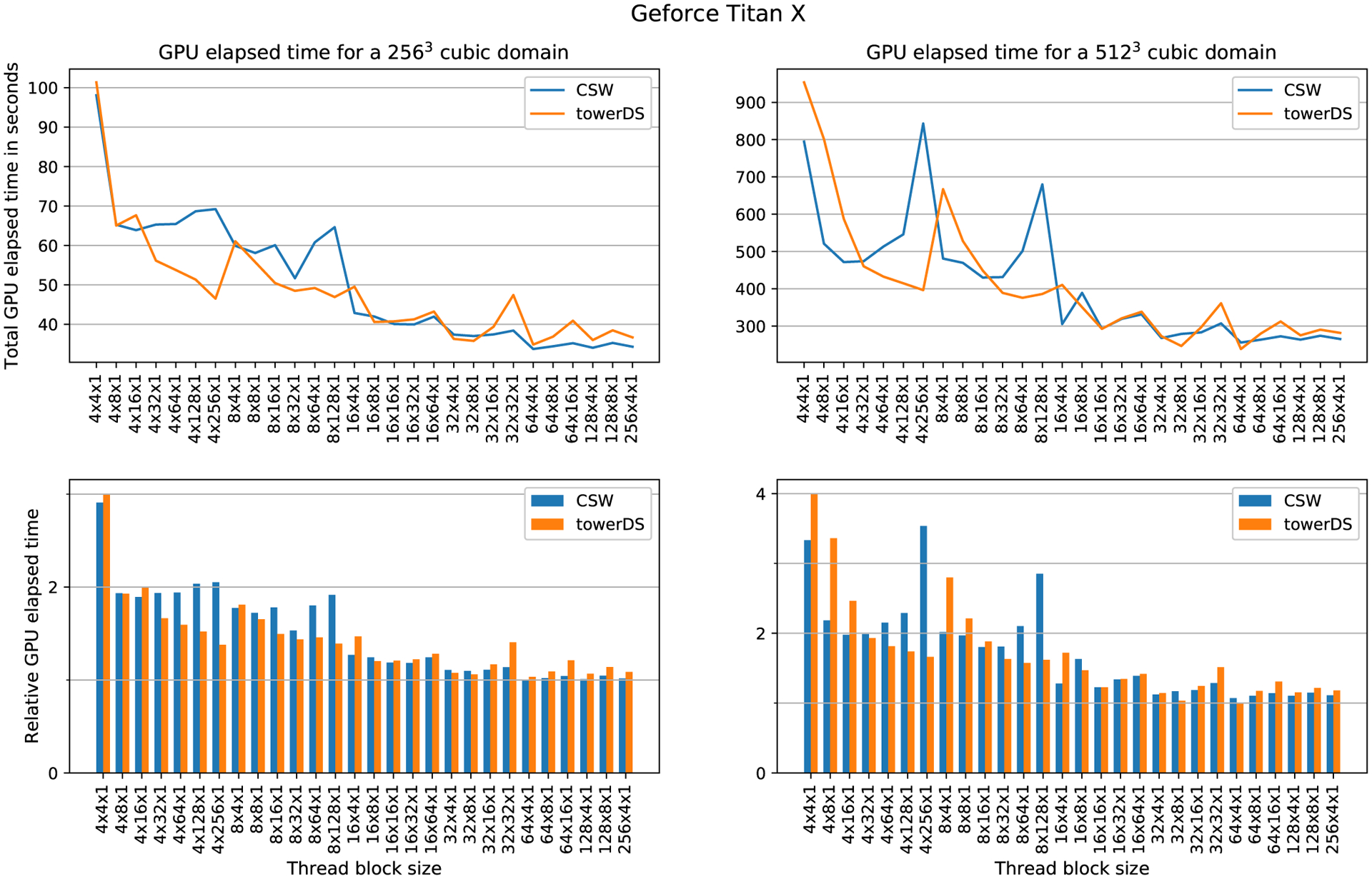
Computation time as function of block size for GTX Titan X. This experiment computed 20 000 time steps

REFERENCES

- 1.Patterson D, Anderson T, Cardwell N, et al. A case for intelligent RAM. IEEE Micro. 1997;17(2):34–44. [Google Scholar]
- 2.Patterson DA, Hennessy JL. Computer Organization and Design. Cambridge, MA: Morgan Kaufmann; 2007:474–476. [Google Scholar]
- 3.Whaley RC, Dongarra JJ. Automatically tuned linear algebra software. In: Proceedings of the 1998 ACM/IEEE Conference on Supercomputing; 1998; Orlando, FL. [Google Scholar]
- 4.Dongarra J Sparse matrix storage formats. Templates for the Solution of Algebraic Eigenvalue Problems: A Practical Guide. Philadelphia, PA: SIAM; 2000:445–448. [Google Scholar]
- 5.Silva J, Boeres C, Drummond L, Pessoa AA. Memory aware load balance strategy on a parallel branch-and-bound application. Concurr Comput Pract Exp. 2015;27(5):1122–1144. [Google Scholar]
- 6.NVIDIA. CUDA C Best Practices. https://docs.nvidia.com/cuda/cuda-c-best-practices-guide/index.html. 2019. Accessed September 25, 2016.
- 7.Michéa D, Komatitsch D. Accelerating a three-dimensional finite-difference wave propagation code using GPU graphics cards. Geophys J Int. 2010;182(1):389–402. [Google Scholar]
- 8.Abdelkhalek R, Calandra H, Coulaud O, Latu G, Roman J. Fast seismic modeling and reverse time migration on a graphics processing unit cluster. Concurr Comput Pract Exp. 2012;24(7):739–750. [Google Scholar]
- 9.Porter-Sobieraj J, Cygert S, Kikoła D, Sikorski J, Słodkowski M. Optimizing the computation of a parallel 3D finite difference algorithm for graphics processing units. Concurr Comput Pract Exp. 2015;27(6):1591–1602. [Google Scholar]
- 10.Clayton RH, Panfilov AV. A guide to modelling cardiac electrical activity in anatomically detailed ventricles. Prog Biophys Mol Biol. 2008;96(1–3):19–43. Cardiovascular Physiome. [DOI] [PubMed] [Google Scholar]
- 11.Bartocci E, Cherry EM, Glimm J, Grosu R, Smolka SA, Fenton FH. Toward real-time simulation of cardiac dynamics. In: Proceedings of the 9th International Conference on Computational Methods in Systems Biology; 2011; Paris, France. [Google Scholar]
- 12.Beeler GW, Reuter H. Reconstruction of the action potential of ventricular myocardial fibres. J Physiol. 1977;268(1):177–210. [DOI] [PMC free article] [PubMed] [Google Scholar]
- 13.Karma A Spiral breakup in model equations of action potential propagation in cardiac tissue. Phys Rev Lett. 1993;71:1103–1106. [DOI] [PubMed] [Google Scholar]
- 14.Iyer V, Mazhari R, Winslow RL. A computational model of the human left-ventricular epicardial myocyte. Biophysical Journal. 2004;87(3):1507–1525. [DOI] [PMC free article] [PubMed] [Google Scholar]
- 15.Tusscher KHWJ Panfilov AV. Alternans and spiral breakup in a human ventricular tissue model. Am J Physiol Heart Circ Physiol. 2006;291(3):H1088–H1100. [DOI] [PubMed] [Google Scholar]
- 16.Bueno-Orovio A, Cherry EM, Fenton FH. Minimal model for human ventricular action potentials in tissue. J Theor Biol. 2008;253(3):544–560. [DOI] [PubMed] [Google Scholar]
- 17.O’Hara T, Virág L, Varró A, Rudy Y. Simulation of the undiseased human cardiac ventricular action potential: model formulation and experimental validation. PLOS Comput Biol. 2011;7(5):1–29. [DOI] [PMC free article] [PubMed] [Google Scholar]
- 18.Hoffman JD, Frankel S. Numerical Methods for Engineers and Scientists. Boca Raton, FL: CRC Press; 2001. [Google Scholar]
- 19.Micikevicius P 3D finite difference computation on GPUs using CUDA. In: Proceedings of 2nd Workshop on General Purpose Processing on Graphics Processing Units; 2009; Washington, DC. [Google Scholar]
- 20.Nimmagadda VK, Akoglu A, Hariri S, Moukabary T. Cardiac simulation on multi-GPU platform. J Supercomput. 2012;59(3):1360–1378. [Google Scholar]
- 21.Giles M, László E, Reguly I, Appleyard J, Demouth J. GPU implementation of finite difference solvers. In: Proceedings of the 7th Workshop on High Performance Computational Finance; 2014; New Orleans, LA. [Google Scholar]
- 22.Harris M Nvidia developer blog: parallel for all. http://docs.nvidia.com/cuda/cuda-c-programming-guide/. Accessed 2013.
- 23.Sanders J, Kandrot E. Cuda by Example: An Introduction to General-Purpose GPU Programming. Boston, MA: Addison-Wesley Professional; 2010. [Google Scholar]
- 24.Niederer S, Mitchell L, Smith N, Plank G. Simulating human cardiac electrophysiology on clinical time-scales. Front Physiol. 2011;2(14). [DOI] [PMC free article] [PubMed] [Google Scholar]
- 25.Mirin AA, Richards DF, Glosli JN, et al. Toward real-time modeling of human heart ventricles at cellular resolution: Simulation of drug-induced arrhythmias. In: Proceedings of the International Conference on High Performance Computing, Networking, Storage and Analysis; 2012; Salt Lake City, UT. [Google Scholar]
- 26.Richards DF, Glosli JN, Draeger EW, et al. Towards real-time simulation of cardiac electrophysiology in a human heart at high resolution. Comput Methods Biomech Biomed Eng. 2013;16(7):802–805. [DOI] [PubMed] [Google Scholar]
- 27.Chai J, Hake J, Wu N, et al. Towards simulation of subcellular calcium dynamics at nanometre resolution. Int J High Perform Comput Appl. 2015;29(1):51–63. [Google Scholar]
- 28.Dematté L, Prandi D. GPU computing for systems biology. Brief Bioinform. 2010;11(3):323–333. [DOI] [PubMed] [Google Scholar]
- 29.Nobile MS, Cazzaniga P, Tangherloni A, Besozzi D. Graphics processing units in bioinformatics, computational biology and systems biology. Brief Bioinform. 2017;18(5):870–885. [DOI] [PMC free article] [PubMed] [Google Scholar]
- 30.Szafaryn LG, Skadron K, Saucerman JJ. Experiences accelerating MATLAB systems biology applications. Paper presented at: The 36th International Symposium on Computer Architecture; 2009; Austin, Texas. https://pdfs.semanticscholar.org/692a/3f0a2c0bb129ff71c3f32dabf2c5f71d7166.pdf [Google Scholar]
- 31.Clayton RH, Bernus O, Cherry EM, et al. Models of cardiac tissue electrophysiology: progress, challenges and open questions. Prog Biophys Mol Biol. 2011;104(1–3):22–48. [DOI] [PubMed] [Google Scholar]
- 32.Lopez-Perez A, Sebastian R, Ferrero JM. Three-dimensional cardiac computational modelling: methods, features and applications. BioMedical Engineering OnLine. 2015;14(1):1–31. [DOI] [PMC free article] [PubMed] [Google Scholar]
- 33.Higham J, Aslanidi O, Zhang H. Large speed increase using novel GPU based algorithms to simulate cardiac excitation waves in 3D rabbit ventricles. Paper presented at: 2011 Computing in Cardiology; 2011; Hangzhou, China. [Google Scholar]
- 34.Mena A, Rodriguez JF. Using graphic processor units for the study of electric propagation in realistic heart models. Paper presented at: 2012 Computing in Cardiology; 2012; Krakow, Poland. [Google Scholar]
- 35.Vigueras G, Roy I, Cookson A, Lee J, Smith N, Nordsletten D. Toward GPGPU accelerated human electromechanical cardiac simulations. Int J Numer Methods Biomed Eng. 2014;30(1):117–134. [DOI] [PMC free article] [PubMed] [Google Scholar]
- 36.Rocha BM, Campos FO, Amorim RM, Plank G, dos Santos RW, Liebmann M, Haase G. Accelerating cardiac excitation spread simulations using graphics processing units. Concurr Comput Pract Exp. 2011;23(7):708–720. [Google Scholar]
- 37.Xia Y, Wang K, Zhang H. Parallel optimization of 3D cardiac electrophysiological model using GPU. Comput Math Methods Med. 2015;2015:1–10. [DOI] [PMC free article] [PubMed] [Google Scholar]
- 38.Mena A, Ferrero JM, Matas JFR. GPU accelerated solver for nonlinear reaction–diffusion systems. Application to the electrophysiology problem. Comput Phys Commun. 2015;196:280–289. [Google Scholar]
- 39.Esmaili E, Akoglu A, Ditzler G, Hariri S, Moukabary T, Szep J. Autonomic management of 3D cardiac simulations. Paper presented at: 2017 International Conference on Cloud and Autonomic Computing (ICCAC); 2017; Tucson, AZ. [Google Scholar]
- 40.Vincent KP, Gonzales MJ, Gillette AK, et al. High-order finite element methods for cardiac monodomain simulations. Front Physiol. 2015;6:217. [DOI] [PMC free article] [PubMed] [Google Scholar]
- 41.Campos JO, Oliveira RS, dos Santos RW, Rocha BM. Lattice Boltzmann method for parallel simulations of cardiac electrophysiology using GPUs. J Comput Appl Math. 2016;295:70–82. VIII Pan-American Workshop in Applied and Computational Mathematics. [Google Scholar]
- 42.Amorim RM, dos Santos RW. Solving the cardiac bidomain equations using graphics processing units. J Comput Sci. 2013;4(5):370–376. [Google Scholar]
- 43.Shewchuk JR. An introduction to the conjugate gradient method. https://www.cs.cmu.edu/quake-papers/painless-conjugate-gradient.pdf. 1994. Accessed January 10, 2018.
- 44.Succi S The Lattice Boltzmann Equation: For Fluid Dynamics and Beyond. Oxford, UK: Oxford University Press; 2001. [Google Scholar]
- 45.Luo CH, Rudy Y. A model of the ventricular cardiac action potential. depolarization, repolarization, and their interaction. Circulation Research. 1991;68(6):1501–1526. [DOI] [PubMed] [Google Scholar]
- 46.Kaboudian A, Cherry EM, Fenton FH. Real-time interactive simulations of large-scale systems on personal computers and cell phones: toward patient-specific heart modeling and other applications. Science Advances. 2019;5(3). [DOI] [PMC free article] [PubMed] [Google Scholar]