A scanner-specific framework for simulating CT images with tube current modulation

Abstract

Although tube current modulation (TCM) is routinely implemented in modern computed tomography (CT) scans, no existing CT simulator is capable of generating realistic images with TCM. The goal of this study was to develop such a framework to (1) facilitate patient-specific optimization of TCM parameters and (2) enable future virtual imaging trials (VITs) with more clinically realistic image quality and x-ray flux distributions. The framework was created by developing a TCM module and integrating it with an existing CT simulator (DukeSim). The developed module utilizes scanner-calibrated TCM parameters and two localizer radiographs to compute the mAs for each simulated CT projection. This simulation pipeline was validated in two parts. First, DukeSim was validated in the context of a commercial scanner with TCM (SOMATOM Force, Siemens Healthineers) by imaging a physical CT phantom (Mercury, Sun Nuclear) and its computational analogue. Second, the TCM module was validated by imaging a computational anthropomorphic phantom (ATOM, CIRS) using DukeSim with real and module-generated TCM profiles. The validation demonstrated DukeSim’s realism in terms of noise magnitude, noise texture, spatial resolution, and image contrast (with average differences of 0.38%, 6.31%, 0.43%, and −9 HU, respectively). It also demonstrated the TCM module’s realism in terms of projection-level mAs and resulting noise magnitude (2.86% and −2.60%, respectively). Finally, the framework was applied to a pilot VIT simulating images of three computational anthropomorphic phantoms (XCAT, with body mass indices (BMIs) of 24.3, 28.2, and 33.0) under five different TCM settings. The optimal TCM for each phantom was characterized based on various criteria, such as minimizing mAs or maximizing image quality. ‘Very Weak’ TCM minimized noise for the 24.3 BMI phantom, while ‘Very Strong’ TCM minimized noise for the 33.0 BMI phantom. This illustrates the utility of the developed framework for future optimization studies of TCM parameters and, more broadly, large-scale VITs with scanner-specific TCM.

1. Introduction

Modern computed tomography (CT) scanners routinely utilize tube current modulation (TCM) to improve image quality while minimizing radiation dose to patients. With TCM, x-ray flux is more proficiently distributed across the patient as the tube current is adjusted according to the varying attenuations and radiosensitivities of each anatomical region. This produces a more uniform noise level across projection images, thus reducing artifacts in reconstructed images without necessitating increased radiation exposure. For this reason, TCM is a common element in clinical CT imaging protocols.

This general concept of TCM is straightforward, but specific approaches and implementations vary across manufacturers, such as GE’s AutomA, Philips’s Dose-Right Dose Modulation, Toshiba’s Real E.C., and Siemens’s CARE Dose 4D (Kalra et al 2004). Within each of these methods, there are additional manufacturer-specific protocol options and settings to choose, such as noise index, image quality reference, and modulation strength (McCollough et al 2006, Li et al 2014), with inherent adaptation to the patient’s body habitus, the anatomy of interest, and the diagnostic task. Given this multiplicity of variables, TCM should ideally be tailored for each patient in order to achieve its optimal use. This requires robust evaluation of TCM in clinical settings, ideally by imaging of a population of diverse patients repeatedly at multiple TCM settings. Such a study is not practical using real patients. Not only would this be expensive and time-consuming, it would place human patients at unacceptable risk due to repeated radiation exposure.

Virtual imaging trials (VITs), which involve the use of computational phantoms and imaging simulators, offer a promising alternative to traditional imaging trials (Abadi et al 2020). By using computational models of humans (virtual patients) and imaging systems (virtual scanners) to model the image acquisition process, VITs bypass the ethical and financial costs of real clinical trials. Moreover, VITs possess unique advantages over traditional trials. With a computational patient, the exact anatomical and material properties are known prior to imaging, enabling more accurate assessment of diagnostic predictions. Using a simulated scanner, images may be generated repeatedly under various settings, with or without noise, facilitating computation of noise profiles and estimation of ensemble noise. The utility of a VIT platform, however, hinges on its clinical realism, including accurate modeling of TCM.

The objective of this study was to develop a validated, scanner-specific framework to simulate CT images with TCM. We aimed to do so by creating a TCM module and integrating it with DukeSim, an established hybrid simulator developed for rapid x-ray imaging of the 4D extended cardiac-torso (XCAT) phantoms (Abadi et al 2019a, 2019b, Sharma et al 2019, Sharma et al 2021). DukeSim accounts for several scanner-specific elements, including scanner geometry, poly-energetic source spectrum, bowtie filtration, anti-scatter grid, flying focal spot, and energy-dependent detector response. The TCM model was integrated with DukeSim in a modular fashion, facilitating flexible integration of the TCM module with different simulation platforms and easy updates to the employed TCM methodology in step with advances in CT imaging.

2. Method

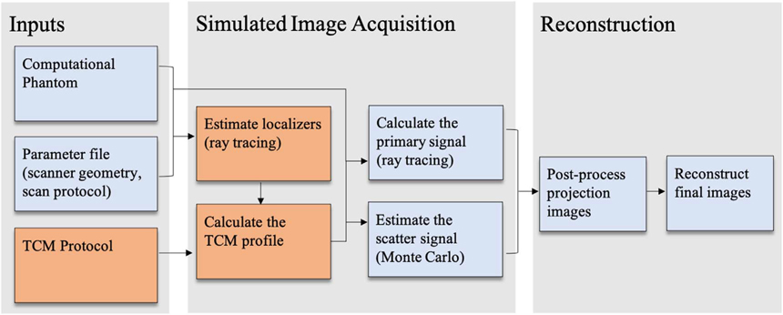
DukeSim generates realistic, scanner-specific CT images from two main inputs: (1) a high-resolution computational phantom and (2) a parameter file defining the scanner-specific geometry and the exam protocol. This work expanded upon this existing framework by incorporating a TCM module, summarized in figure 1. The following subsections describe the TCM model’s development, manufacturer-specific calibration, validation, and application in a pilot VIT.

Figure 1.

Flowchart summarizing DukeSim’s simulation framework. TCM-specific elements are shown in orange.

2.1. Model development

TCM operates based on the general principle of adjusting tube current to accommodate varied x-ray attenuation across projections, but the precise details of manufacturer-specific implementations are often proprietary. Realistic models may be estimated by calibrating a general model to data acquired from real acquisitions. For this implementation, we primarily focused on Siemens’s method, CARE Dose 4D (CD4D) (Flohr 2011). With CD4D, the user first selects a TCM strength and protocol based on the anatomy of interest, and the software computes a TCM profile based on the patient’s estimated attenuation. During the exam, additional attenuation measurements are made, and the TCM profile is refined ‘on-line.’ Based on this understanding of CD4D, we aimed to precisely model its known methodological elements and to estimate its unknown proprietary elements, with the goal of producing realistic TCM profiles in DukeSim.

2.1.1. Generic attenuation-based TCM

The human body is inhomogeneous and asymmetric, so if a CT scan uses a constant tube current, the number of photons detected for each projection image will vary considerably. Since quantum noise is known to be inversely proportional to the square root of the number of photons hitting the detector, the noise level across projections is expected to be nonuniform. This nonuniformity can cause reconstructed images to suffer from photon starvation and larger noise amplitudes in certain directions (Kalender et al 1999). One goal of TCM is to minimize these directional noisy artifacts without increasing the total patient dose.

For an air scan, the number of photons hitting the detector is a function of the effective mAs,

$$mAs=\frac{m{A}^{*}{T}_{rot}}{pitch},$$ (1)

where mA is the tube current in milliamperes, T_rot is the gantry rotation time in seconds, and pitch is the ratio of table feed per rotation to beam collimation. With the addition of a patient, the number of photons reaching the detector is further reduced by the attenuation for each projection. Thus, an attenuation-based mAs modulation may be introduced as

$$mAs(p)=mA{s}_{\text{ref}}{\left(\frac{A(p)}{A_{\text{ref }}}\right)}^{\alpha },$$ (2)

where mAs (p) is the TCM profile as a function of projection p, mAs_ref is the reference mAs, A (p) is the characteristic attenuation as a function of projection p, A_ref is the reference attenuation, and α is the modulation strength parameter between 0 and 1.

Past studies have verified this model for multiple manufacturers by demonstrating that the logarithm of the tube current is linearly proportional to phantom diameter (Flohr 2011, Li et al 2014). Furthermore, different α values may be tailored to different purposes. For example, α = 1 is meant to achieve a constant noise level, while α = 0.5 minimizes noise in the central pixel of each projection when imaging an elliptical, uniform-material phantom (Gies et al 1999). However, both of these are highly idealized scenarios. Aiming for constant noise in all clinical situations will result in unnecessary radiation dose for large patients, and human patients are neither elliptical nor homogeneous (Flohr 2011, Favazza et al 2015). For this reason, a manufacturer may choose to provide multiple α options for different protocols. This is the case with CD4D, which offers five TCM strength options.

2.1.2. Manufacturer-specific TCM

With CD4D, the constants A_ref and α depend on the protocol selected by the user. Prior to each scan, the user chooses an anatomy of interest, adult or pediatric, and one of five strengths (very weak, weak, average, strong, and very strong). A_ref depends on the anatomy chosen, while α is unique to each TCM strength and differs between adult and pediatric patients. The quantity α is further split into two values for slim and obese patients, α_slim and α_obese (Favazza et al 2015, McMillan et al 2017), which are implemented for attenuations A (p) < A_ref and A (p) > A_ref, respectively. There are some protocol exceptions which utilize a unique (α_slim, α_obese) pair for each TCM strength, for example the neck protocol. For this study, we focused on the thorax and abdomen protocols.

Additionally, TCM is commonly comprised of two components: longitudinal TCM (along the craniocaudal, z-axis of the patient) and angular TCM (within a single rotation of the x-ray tube, in the x–y plane) (Kalra et al 2004). Certain CD4D protocols, such as the head protocol, exclusively employ longitudinal modulation (Jian and Ma Hao 2007). Other protocols utilize both longitudinal and angular modulations, especially in areas with high degrees of rotational asymmetry (such as thorax and abdomen protocols).

2.2. Simulation implementation

We calibrated DukeSim’s α_slim and α_obese to the five TCM strengths available with CD4D. In doing so, it was necessary to develop a method for estimating the patient attenuation profile, A (p). For all protocols, CD4D typically estimates A (p) from a single localizer radiograph, either anterior–posterior (AP) or lateral (Lee et al 2008). With longitudinal TCM, this is straightforward to emulate. Each patient cross-section is approximated as a circle, and the water-equivalent diameter is computed for each row (Zhang et al 2020). However, for protocols which incorporate angular TCM, CD4D utilizes an algorithm to compute the attenuation in the perpendicular view (Rego et al). The details of this method are proprietary, so we instead developed our module to utilize two simulated localizer radiographs and directly measure the attenuation profile of both.

2.2.1. TCM module

The developed TCM module utilizes a user-defined parameter file with scanner geometry and two localizer radiographs to generate a projection-level mAs profile. The two localizers may be simulated with DukeSim prior to running the module.

To simulate any CT acquisition, DukeSim’s geometry and physics are first set according to the scanner parameter file. When simulating a localizer radiograph, the tube current-time product is changed to 35 mAs and the beam collimation and distance of gantry travel per rotation are reduced to the size of a single pixel row (Hoye et al 2019). With these settings, a single localizer sinogram μL is acquired. This method is repeated at the AP view and the lateral view to generate the two localizers needed for the TCM module. Then, the water-equivalent length vectors L_w,AP (z) and L_w,LAT (z) are calculated as

$$L_w(z)=\frac{\max (\mu L(z:z+dz))}{{\mu }_w},$$ (3)

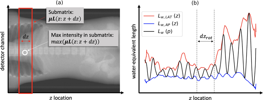
where μ_w is the linear attenuation coefficient of water, z is the location of the central row of each projection, dz is a function of the beam collimation implemented to account for the multiple detector rows, and μL (z: z + dz) is the submatrix including rows in the range z to z + dz and all detector channels (as illustrated in figure 2(a)).

Figure 2.

Schematic diagram illustrating the process of converting two localizer radiographs into one projection-level water-equivalent length profile. (a) An example localizer μL_AP is shown with one submatrix μL(z: z + dz) boxed in red and its maximum intensity max (μL(z: z + dz)) circled in white. (b) The vectors L_w,LAT (z) and L_w,AP (z) are used to compute L_w (p) for a predefined dz_rot and an initial tube angle ϕ = 0.

The angular attenuation profile is approximated using the method described by Kalendar et al oscillating sinusoidally between the maximum and minimum expected attenuations for each rotation (Gies et al 1999). These typically occur at the lateral and AP views respectively, so L_w,AP (z) and L_w,LAT (z) are used to generate this projection-level water-equivalent length profile L_w (p) as

$$L_w(p)=L_{w,AP}(z)+\frac{L_{w,LAT}(z)-L_{w,AP}(z)}{2}\left(1+\cos \left(\frac{4\pi z}{d{z}_{\text{rot}}}+2\varphi \right)\right),$$ (4)

where dz_rot is the distance of gantry travel per rotation and ϕ is the initial tube angle, such that ϕ = 0 corresponds to the lateral view (as illustrated in figure 2(b)).

Finally, a reference attenuation and (α_slim, α_obese) pair are selected to correspond to the desired strength setting. Equation (2) is utilized to calculate the mAs as a function of L_w for each projection p,

$$mAs(p)=mA{s}_{\text{ref}}\left(e^{\alpha {\mu }_w\left(L_w(p)-L_{\text{ref}}\right)}\right),$$ (5)

where L_ref is the reference length equivalent to ln(A_ref)/μ_w. The L_w (p) is input to equation (5), producing a projection-level TCM profile mAs (p) which includes both longitudinal and angular TCM components. Maximum and minimum mAs limits are imposed in accordance with the manufacturer’s known tube power limits. This final TCM profile is used as input to the CT simulator.

2.2.2. CT simulator

To simulate the image acquisition process, DukeSim uses a GPU-accelerated hybrid of ray-tracing and Monte Carlo (MC) techniques as described by Abadi et al (2019a). In summary, for each projection, the primary signal is calculated by solving for attenuation at each detector pixel from the Beer–Lambert law. To model the finite sizes of the source and detector pixels, each is sub-sampled 5 times and the result at each pixel averaged across the 25 combinations. The scatter signal is estimated from the MC simulation, normalized to be per 1 mAs, and added to the raw primary signal. The mAs value for the projection is assigned based on the TCM profile generated prior to each scan (as described in section 2.2.1) and used to determine the final magnitude and noise of the total signal. Finally, a 4th-degree polynomial water correction is applied to the raw sinogram to calibrate HU values and alleviate effects due to beam hardening, and a scanner-specific signal-dependent filter, provided by the manufacturer, is applied to reduce noise magnitude in regions of low signal.

2.3. Simulated TCM calibration

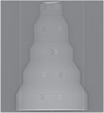
To determine the five (α_slim, α_obese) pairs for DukeSim when simulating CD4D, calibration data were acquired by imaging a variable-sized physical phantom (Mercury, Sun Nuclear) on a representative scanner (SOMATOM Force, Siemens Healthineers) at multiple strength settings. The phantom consisted of five cylindrical polyethylene sections of increasing diameter (12.0, 18.5, 23.0, 30.0, and 37.0 cm). Each section included a sub-region with five material inserts (water, bone, polystyrene, iodine, and air) to facilitate evaluation of contrast.

The phantom was scanned at 120 kV using a standard ‘body’ bowtie filter, diagonal flying focal spot, helical pitch factor of 0.6, rotation time of 0.5 s, and the ‘abdomen’ protocol. Fifteen scans were completed in total, using all five available TCM strength options and three different reference mAs values of 50, 100, and 200. The dataset included a localizer radiograph with a private DICOM header containing water-equivalent length estimates at both the AP and lateral views as a function of longitudinal location z, or L_w,AP (z) and L_w,LAT (z), respectively (McMillan et al 2014, McMillan et al 2017). This was used as input to equation (4) to generate the angular water-equivalent length profile L_w (p).

For each of the fifteen scans, a full TCM profile mAs (p) was obtained by extracting the mAs value from the header of each raw projection image. Each profile was divided by its reference mAs, producing five normalized datasets corresponding to the available TCM strengths. The five (α_slim, α_obese) pairs were found by fitting these data points L_w (p), mAs (p) to equation (5) and minimizing the root mean square error (RMSE) in units of normalized mAs. The slim data L_w (z) < L_ref were used for α_slim, and the remaining data with L_w (z) > L_ref were used for α_obese. Extreme data points (i.e. those limited by the minimum and maximum x-ray tube power limits) were excluded from the data fitting, since these points do not reflect the expected output of equation (5) and are instead found by imposing limits to the mAs range.

2.4. Simulation validation

A validation study was completed in two steps to demonstrate the realism of images simulated with DukeSim at multiple TCM settings. First, the simulator was evaluated by comparing real images to simulated images generated with the same projection-level mAs profile. Second, the TCM module was evaluated by comparing simulated images with real mAs profiles to simulated images with DukeSim mAs profiles. The image acquisition settings are detailed below in table 1.

Table 1.

Summary of the scan configurations used for the image acquisitions described below.

	TCM calibration/simulator evaluation	TCM module evaluation	Pilot VIT
Scanner	Force, DukeSim	DukeSim	DukeSim
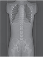
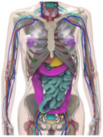
Phantom	Mercury	ATOM (adult, male)	XCAT (BMIs of 24.3, 28.2, and 33.0)
Source of TCM profiles	CD4D	CD4D, DukeSim	DukeSim
mAsref	50, 100, 200	100	100
Average CTDIvol (mGy per mAs)	2.36, 4.52, 8.92 (for each mAsref)	3.77, 3.98 (for each TCM profile)	7.27, 10.01, 14.02 (for each phantom)
TCM strength	Very weak, weak, average, strong, very strong	Average	Very weak, weak, average, strong, very strong
Lref (cm)	33.9	33.9	31.4
Helical pitch	0.6	0.6	1.0

2.4.1. Simulator evaluation—methods

A computational version of the Mercury phantom was scanned with DukeSim set to model the geometry and physics of the SOMATOM Force (Siemens Healthineers). Protocol settings matched those of the earlier data acquisition (120 kV spectrum, helical pitch of 0.6, diagonal flying focal spot, rotation time of 0.5 s). The fifteen real TCM profiles were registered to the computational Mercury phantom and used as input to DukeSim. Both real and simulated projection images were reconstructed using an offline reconstruction prototype (ReconCT 15.0.35098.0, Siemens Healthineers) with a weighted filtered backprojection algorithm (WFBP, kernel of Br40d), matrix size of 512, 400 mm field of view, and 0.6 mm slice thickness.

Noise metrics were measured in the reconstructed images by placing eight square regions of interest (ROIs) in the homogeneous polyethylene region of each cylinder. Each ROI had side length of 25 mm and was located 40 mm away from the phantom center. Noise magnitude was computed as the average standard deviation of HU values, and noise power spectrum (NPS) was computed using the method described by Solomon et al (2015). The in-plane modulation transfer function (MTF) was measured for the high-contrast material inserts (air and bone). Contrast was measured as mean CT number for all five material inserts (air, iodine, polystyrene, bone, water). All metrics were averaged across 15 consecutive slices.

2.4.2. TCM module evaluation—methods

A physical adult male ATOM phantom (Computerized Imaging Reference Systems, CIRS) was imaged on a SOMATOM Force scanner (Siemens Healthineers) (ATOM® Dosimetry Phantoms 2013). Unlike the Mercury phantom, the ATOM phantom is anthropomorphic and thus the TCM profile must account for attenuation inhomogeneities typical of a real patient. The phantom was imaged at 120 kV using a ‘body’ bowtie filter, diagonal flying focal spot, helical pitch factor of 0.6, rotation time of 0.5 s, and ‘abdomen’ protocol. One scan was conducted with 100 mAs_ref and ‘Average’ strength. The TCM profile mAs_real (p) was found by extracting the mAs from the header for each raw projection image.

A module-generated TCM profile mAs_DukeSim (p) was calculated using the water-equivalent length vectors L_w,AP (z) and L_w,LAT (z) extracted from the DICOM header of the localizer. The projection-level attenuation profile L_w (p) was computed from equation (4), and a final TCM profile mAs_DukeSim (p) was calculated from equation (5).

To quantify the effect of differences between the real TCM profile and simulated TCM profile, DukeSim was used to simulate images of a computational version of the adult male ATOM phantom using the two mAs vectors. The geometry and physics were set to model the SOMATOM Force scanner at the same acquisition settings listed above, with and without simulated noise. Images were reconstructed in ReconCT with a WFBP algorithm (kernel of Br40d), 1024 matrix size, 500 mm field of view, and 0.6 mm slice thickness. A noise profile was computed for each dataset by subtracting the noiseless reconstructed images from the noisy reconstructed images and taking the absolute value. Noise magnitude was measured in each reconstructed slice as the mean value of the corresponding noise profile slice. The mAs for each slice was defined as the average of the mAs used for the projection images in that reconstruction.

2.4.3. Pilot VIT—methods

To illustrate the utility of this framework, a pilot VIT was conducted to quantify image quality as a function of TCM strength for patients of different sizes.

DukeSim was used to simulate images of three adult male XCAT phantoms at all five modeled TCM strengths, with and without noise. The three phantoms included textured lungs and bones and had body mass indices (BMIs) of 24.3, 28.2, and 33.0 (25th, 50th, and 75th percentile of the US adult population, respectively). The geometry and physics of DukeSim were set to model the SOMATOM Force scanner at 120 kV using ‘body’ bowtie filter, helical pitch factor of 1.0, rotation time of 0.5 s, and diagonal flying focal spot. For TCM, the ‘thorax’ protocol was used (reference length of 31.4 cm) with mAs_ref of 100.

The simulated projection images were reconstructed using ReconCT with a weighted filtered backprojection algorithm (kernel of Br40d), matrix size of 1024, 500 mm field of view, and slice thickness of 0.6 mm. Noise magnitude was measured in each reconstructed slice, and average noise magnitude and average mAs delivered were calculated in lungs and bones. Noise metrics were found using the method described in section 2.4.2, and the average mAs delivered was found by registering the CT images to the original XCAT phantoms, then computing the mean mAs of the CT slices weighted by the number of organ voxels in each slice.

3. Results

3.1. TCM Calibration

Figure 3 shows the calibration data and curve fit results for the five TCM strengths. The (α_slim, α_obese) pairs and RMSEs are listed in table 2. The RMSE ranged from 4.2% to 6.6% for the slim data and 8.4% to 17.5% for the obese data, showing reasonable agreement between DukeSim’s model and CD4D data. As L_w increased, noise in mAs also increased, contributing to the greater RMSE for obese data.

Figure 3.

Normalized mAs as a function of water-equivalent length for all five TCM strengths. DukeSim calibration curves are plotted with RMSE as error bars. A vertical gray line is shown at the reference length, 33.9 cm.

Table 2.

TCM curve fitting results. Each pair of parameters was found by minimizing RMSE (units of normalized mAs) for slim and obese data.

TCM strength	α slim	α obese	RMSEslim	RMSEobese
Very weak	0.236	0.202	0.066	0.084
Weak	0.393	0.241	0.057	0.084
Average	0.606	0.360	0.042	0.090
Strong	0.759	0.497	0.044	0.124
Very strong	0.913	0.674	0.051	0.175

3.2. Validation

3.2.1. Simulator evaluation—results

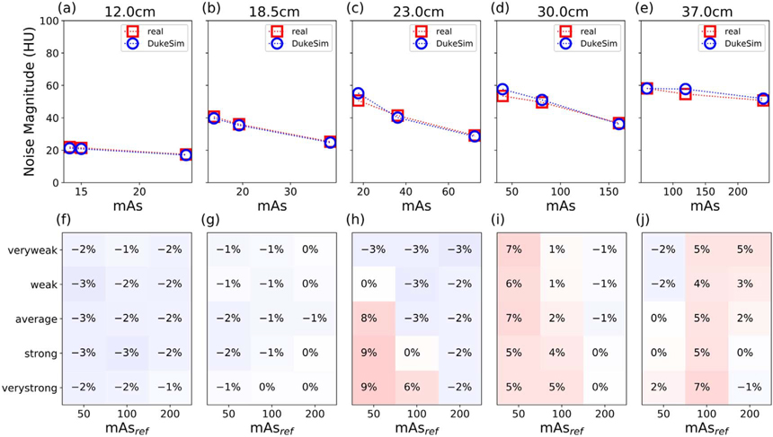
In figure 4, the first row (a)–(e) shows real and simulated noise magnitude (NM) for data with Average TCM and three mAs_ref. As expected, noise magnitude decreased with mAs (for a given size), and increased with size (for a given mAs) in both real and simulated images. In the large-diameter regions of the phantom when imaged with low mAs, noise did not follow the traditional relationship NM ∝ mAs^−0.5. This is due to the adaptive filter applied to low-signal data to improve image quality when scanning highly-attenuating objects at low doses (Kachelrieß et al 2001). The second row (f)–(i) shows relative error for all five TCM strengths and three mAs_ref. The relative error was within ±9% for each dataset and on average 0.38%, demonstrating realistic simulated noise magnitude.

Figure 4.

(a)–(e) Noise magnitude comparison for one TCM strength (Average) at three reference mAs (50, 100, and 200) in the five Mercury phantom diameters. The mAs of each slice was calculated as the average mAs of projections used in its reconstruction. (f)–(j) Heat map of the relative error in noise magnitude for all five TCM strengths and three reference mAs. Notably, error is typically small (±3%) but increases slightly in the low-dose regime (higher attenuating diameter and lower reference mAs).

Figure 5 shows the 2D NPS measured in the middle (23 cm diameter) section of the Mercury phantom for the real and DukeSim images with 100 mAs_ref. The average frequency (f_avg) and peak frequency (f_peak) of each NPS curve are listed in table 3. NPS did not noticeably vary with TCM strength, likely in part due to the high rotational symmetry of the Mercury phantom. The mean f_avg across TCM strengths was 0.286 mm⁻¹ for real images and 0.311 mm⁻¹ for simulated images (relative error of 8.05%). Likewise, mean f_peak values were 0.239 mm⁻¹ and 0.258 mm⁻¹ respectively (relative error of 6.31%). This demonstrates reasonable agreement in texture between real and simulated images.

Figure 5.

Normalized noise power spectrum (NPS) in the 23 cm diameter cylinder of the Mercury phantom, measured in real (red) and simulated (blue) images for each TCM strength with reference mAs of 100.

Table 3.

Average and peak frequency values of real and simulated NPS (figure 5) at multiple TCM strengths.

TCM strength	Dataset	favg (mm−1)	fpeak (mm−1)
Very weak	Real	0.287	0.189
	DukeSim	0.310	0.283
Weak	Real	0.287	0.252
	DukeSim	0.311	0.252
Average	Real	0.287	0.283
	DukeSim	0.313	0.283
Strong	Real	0.288	0.252
	DukeSim	0.310	0.220
Very strong	Real	0.280	0.220
	DukeSim	0.310	0.252

Figure 6 shows the in-plane MTF measured for the Air and Bone material inserts. For Air, the average frequency at 50% of the maximum (f₅₀) was 0.370 mm⁻¹ in real images and 0.369 mm⁻¹ in simulated images. For bone, these values were 0.362 mm⁻¹ and 0.361 mm⁻¹, respectively. The relative error in f₅₀ was 0.43% for both materials, showing very similar spatial resolution between real and simulated images.

Figure 6.

Modulation transfer function (MTF) of air (a)–(e) and bone (f)–(j) material inserts in the 30 cm diameter section of the Mercury phantom, measured in real (red) and simulated (blue) images at five TCM strengths.

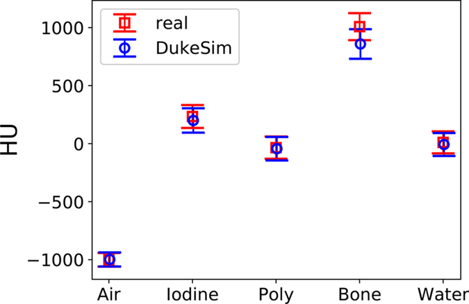
Figure 7 compares the average CT numbers of the five material inserts in real and simulated images (difference of 2.9, −34.0, −8.9, −149.3, and −18.2 HU for air, iodine, polystyrene, bone, and water respectively), showing strong agreement in contrast.

Figure 7.

Mean CT number for the five material inserts in the 23 cm diameter section of the Mercury phantom, for real and simulated data at 100 mAs_ref averaged across multiple TCM strengths (absolute error is 2.9, −34.0, −8.9, −149.3, and −18.2 HU for each material, left to right). Error bars are standard deviation.

3.2.2. TCM module evaluation—results

Figure 8 shows the two TCM profiles generated for the ATOM phantom, mAs_DukeSim (p) and mAs_real (p). The accuracy of the simulated TCM profile may be seen visually and quantitatively, with an average relative error of 2.86%. The resulting noise profiles are also very close in magnitude, with an average relative error of −2.60%. Note that the mAs_ref for these acquisitions was 100, and the average water-equivalent size of the ATOM phantom in the region imaged was 27.5 cm, sufficient to avoid the low-dose imaging regime. The sensitivity of the noise magnitude to changes in TCM profile was quantified by plotting noise difference (DukeSim—real) as a function of mAs difference. For an error of +5 mAs, the noise magnitude changes by approximately −1 HU. This illustrates the accuracy of DukeSim’s TCM in terms of both input mAs and resulting noise magnitude.

Figure 8.

(a) Comparison of real TCM vector and DukeSim-generated TCM vector for ATOM phantom scan with reference mAs of 100, ‘average’ strength, and ‘abdomen’ protocol (RMSE 7.59 mAs, average relative error 2.86%). (Background) localizer radiograph of the ATOM phantom. (b) Noise magnitude in each reconstructed slice of the ATOM phantom images, simulated with real and DukeSim-generated TCM profiles. The RMSE is 0.78 HU, and the average relative error is −2.60%. (c) Difference in noise magnitude as a function of TCM difference. A linear fit is shown in red for approximation of the noise magnitude’s sensitivity (RMSE 0.18 HU).

3.2.3. Pilot VIT—results

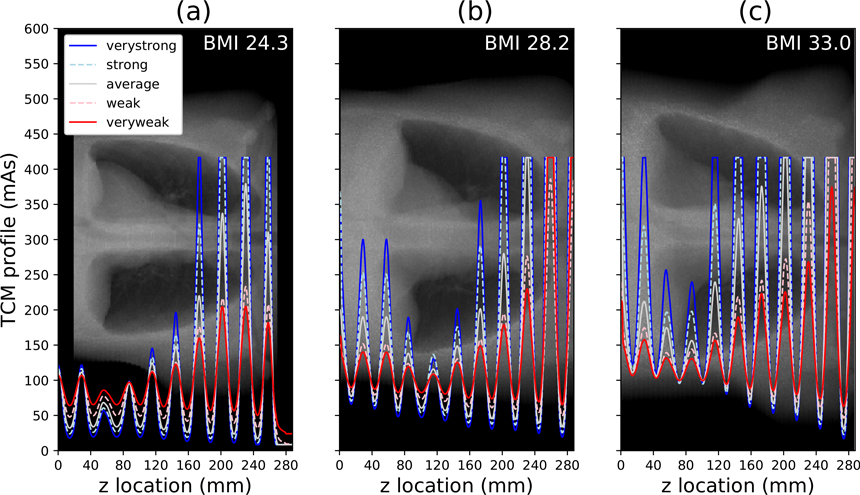
Figure 9 displays the five TCM profiles generated for each of the three XCAT phantoms. The average mAs of each profile increases with phantom size, and the amplitude of angular oscillations increases with TCM strength. Some oscillation peaks have been clipped due to the imposed maximum tube power limit. This is especially apparent for the largest phantom (BMI 33.0), resulting in a convergence of the TCM profiles in some rotations.

Figure 9.

The five TCM profiles generated for each XCAT phantom. The BMI is in 25th, 50th, and 75th percentile of adult males in the United States for (a)–(c) respectively. The profiles are plotted over the corresponding phantom’s AP localizer radiograph.

Figure 10 shows the noise magnitude in each reconstructed slice of the fifteen simulated datasets. For the smallest phantom (BMI 24.3), greater TCM strengths resulted in higher noise magnitude. For the medium-sized phantom (BMI 28.2), the noise profiles were relatively similar regardless of TCM strength. For the largest phantom (BMI 33.0), ‘Very Strong’ TCM resulted in the greatest reduction in noise magnitude.

Figure 10.

Noise magnitude measured in each reconstructed image for the three XCAT phantoms (smallest to largest BMI, left to right).

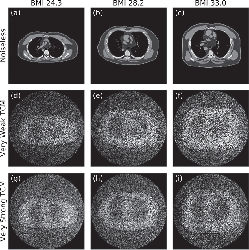
Figure 11 complements the data plotted in figure 10 by showing one noiseless image and two corresponding noise profiles for each phantom. The TCM strength which minimizes noise may be visually identified for each phantom. As expected, ‘Very Strong’ TCM results in a higher-intensity noise profile than ‘Very Weak’ TCM for the smallest phantom, whereas the two noise profiles are similar for the medium-sized phantom, and the trend is opposite for the largest phantom. Additionally, note that noise magnitude clearly increases with phantom BMI for ‘Very Weak’ TCM but is more constant across phantoms for ‘Very Strong’ TCM.

Figure 11.

(a)–(c) Noiseless reconstructed images for the three phantoms (BMIs 24.3, 28.2, and 33.0 from left to right) at window width of 400 HU and a window level of 50 HU. (d)–(f) Corresponding noise profiles for the ‘Very Weak’ TCM simulations. (g)–(i) Corresponding noise profiles for the ‘Very Strong’ TCM simulations. Noise profiles are shown with intensities ranging from 10 to 50 HU. All images are for the central reconstructed slice (z location of 143.1 mm).

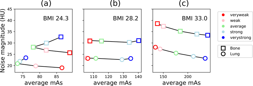
Figure 12 shows organ-specific trends in noise magnitude as a function of the average mAs delivered. In general, the mAs delivered to the bones was higher than that of the lungs, and trends in noise magnitude were similar for both organs. This is expected, due to the higher attenuation of bone. The optimal TCM strength, considering both mAs and noise magnitude, was distinct for each phantom. For the smallest phantom, noise magnitude was minimal for ‘Very Weak’ TCM, while mAs delivered was minimal for ‘Average’ TCM. Interestingly, in the bones, the ‘Strong’ and ‘Weak’ TCM both utilized similar mAs, but ‘Weak’ TCM resulted in lower noise magnitude. For the medium phantom, average mAs delivered ranged from 105 to 140 mAs, but noise magnitude was similar at all TCM strengths. For the largest phantom, noise magnitude monotonically decreased with TCM strength, indicating the best image quality was achieved with ‘Very Strong’ TCM and the lowest mAs delivered was with ‘Very Weak’ TCM.

Figure 12.

Noise magnitude measured in lungs and bones as a function of the average mAs used to acquire projection images with each respective organ, for the three XCAT phantoms.

4. Discussion

VITs show great potential for patient-specific optimization of imaging designs, techniques, and protocols, but only when they are able to realistically simulate clinical imaging scenarios. Prior to this work, no existing VIT framework was capable of simulating CT images with manufacturer-specific TCM. This study developed such a framework. This has the twofold benefit of (1) facilitating future patient-specific optimizations of TCM settings and (2) enabling future VITs with accurate TCM functionality, enhancing the clinical realism of simulated images and dose estimations.

In this study, we modeled one major CT manufacturer’s TCM approach. The exact TCM methodology of most vendors is proprietary, so we demonstrate a simple method for calibrating a generic model to manufacturer-specific TCM parameters using a phantom with regions of distinct attenuations. This may be used to calibrate DukeSim to the TCM methods of other manufacturers, when known to follow the relationship of equation (2). These methods will be incorporated in future studies.

Using the modeled TCM approach (Siemens, CARE Dose 4D), we demonstrated strong agreement between real and simulated images at multiple TCM strengths in terms of noise magnitude, noise texture, contrast, and resolution. For such evaluations, it is critical to use a computational phantom which is faithful to the geometric and physical properties of the real object imaged. It is not possible to have such detailed knowledge of patients, so we utilized a cylindrical physical phantom with various diameters, the Mercury Phantom. This allowed us to assess image quality in well-defined, homogeneous regions and to calibrate our TCM module to simple mAs profiles spanning multiple distinct attenuations. In the context of TCM, the same algorithm is used when generating TCM profiles for simplistic phantoms and for real patients, so we expect our calibration will produce accurate TCM profiles for most cases. We demonstrated this using the anthropomorphic ATOM phantom. Our TCM model produced a highly accurate projection-level mAs profile (±7.6 mAs), and any error in this simulated profile resulted in only small variations in noise magnitude (±0.8 HU) and CTDI_vol (+0.20).

This simulation framework has great potential for further optimizations of TCM settings. Some past studies of TCM have focused on reductions in patient dose with constant image quality (Li et al 2014, Tian et al 2015, McMillan et al 2017), as it is well understood that TCM has a significant impact on x-ray flux distribution and thus dose computation. However, there is limited prior art with regard to variations in image quality, and past attempts at such studies have been limited by simplified physical phantoms, generic simulations, or restricted patient data (Gies et al 1999, Kalender et al 1999, Solomon et al 2013, Gang et al 2017). Ideally, image quality assessments would be conducted through repeat acquisitions of patients at different TCM settings, but this is not possible in real clinical imaging trials. We showed the potential for improved future analyses using our VIT framework with accurate TCM, scanner-specific geometry and physics, and a large library of detailed computational patients.

The prospect of VIT platforms and optimization of TCM relies on the detail and accuracy of anthropomorphic computational phantoms and simulation tools (Abadi et al 2020). In recent years, these have been greatly advanced. On the computational phantom side, the XCAT phantoms have grown into a vast library of male and female patients spanning 1st to 99th percentile BMIs of adults and children in the United States (Segars et al 2010). The XCAT phantoms were recently enhanced to include intra-organ heterogeneities in the lungs, bones, and liver, as well as disease pathologies such as COPD and COVID-19 (Abadi et al 2018, Abadi et al 2019c, Sauer et al 2019, Abadi et al 2021a, 2021b). On the virtual scanner side, simulation platforms have been developed using a variety of methods. MC techniques are often utilized for their accuracy in modeling x-ray interaction physics and estimating delivered radiation dose (Jiang and Paganetti 2004, Li et al 2011, Ding et al 2015). Since pure MC simulations are naturally slow, more recent platforms also utilize GPU-acceleration, ray-tracing, or hybrid (combined ray-tracing and MC) techniques to facilitate assessments of image quality and to use larger patient sample sizes (De Man et al 2007, Badal and Badano 2009, Fung et al 2011, Abadi et al 2019a). In this study, we utilized DukeSim, an established hybrid simulation platform (Abadi et al 2019a, 2019b, Sharma et al 2019, Sharma et al 2021).

In our pilot VIT, we illustrated the patient-specific dependence on image quality as a function of TCM strength for phantoms of varying BMIs. To our knowledge, this is the first instance quantifying this relationship using realistic computational patients. Moreover, we showed example factors to consider in optimization of TCM protocols (noise variations across reconstructed slices, noise magnitude in different organs, average mAs delivered to different organs) and how these may be weighed differently depending on patient anatomy and scan purpose. For example, if considering noise magnitude alone, ‘Very Weak’ TCM is optimal for the 25th percentile BMI patient, while ‘Very Strong’ TCM is optimal for the 75th percentile BMI patient. If considering a particular organ, such as the lungs specifically, ‘Average’ TCM may instead be considered optimal for the 25th percentile BMI patient, since it minimized the mAs delivered with little cost to noise magnitude. This tradeoff is not apparent in all phantoms, further motivating future optimization studies of TCM parameters and showing the ability of this framework to achieve such patient-specific protocols.

This study had some limitations. First, we modeled only an attenuation-based TCM approach. Although outside the scope of this work, more advanced TCM methodologies are increasingly utilized. For example, certain methods utilize dynamic bowtie filters or account for the radiation sensitivity of different organs (Liu et al 2014, Fu et al 2017a, 2017b, Huck et al 2021). Simulation of these will require development of new generic models and calibration methods. Because this framework is modular in nature, the developed TCM module may be easily updated for future simulation studies. Second, our validation of the SOMATOM Force was completed utilizing an established image quality phantom, advantageous for its regions of distinct attenuations and simple geometry. However, real patients do not have circular cross-sections nor homogeneous composition. Unfortunately, it is not yet possible to complete validation using patient images, due to the absence of a known ground truth. Once developed, detailed physical XCAT phantoms with well-defined computational analogues should be used for further validations. Third, for this same reason, our TCM module was validated using only DukeSim-generated images and a computational ATOM phantom. Our aim was simply to approximate the sensitivity of image noise to changes in TCM profile, for which it is necessary to know a phantom’s ground truth and to simulate noiseless images. Our computational ATOM phantom has acceptable accuracy for these purposes. Future analyses should also validate simulated TCM using physical anthropomorphic phantoms with known ground truth. Finally, we validated our simulation framework for typical clinical imaging scenarios, but we found our simulated noise magnitude was less accurate in the low-dose regime. This is because the SOMATOM Force employs adaptive filtration to improve image quality for low-signal projection images. While we have implemented a signal-dependent filter in our simulation framework, our results are still most accurate at more clinically relevant dose levels. This finding motivates a future study modeling a more advanced version of this pre-processing filter in low-signal projections, in order to run accurate VITs at all dose levels.

5. Conclusions

This work demonstrates the first scanner-specific VIT framework which generates realistic CT images with TCM. We validated DukeSim set to model the SOMATOM Force scanner with CARE Dose 4D at all five available TCM strengths. In the future, more advanced TCM methodologies will be modeled and other manufacturers’ implementations will be calibrated. With DukeSim, we are now able to conduct patient-specific optimizations of TCM strengths, as well as more robust VITs which simulate clinical imaging protocols using TCM.

Data availability statement

N.A.

References

- Computerized Imaging Reference Systems, Inc. ATOM® Dosimetry Phantoms. 2013 https://www.cirsinc.com/wp-content/uploads/2021/06/701-706-ATOM-PB-062521.pdf.
- Abadi E. et al. Development of a scanner-specific simulation framework for photon-counting computed tomography. Biomed. Phys. Eng. Express. 2019a;5:055008. doi: 10.1088/2057-1976/ab37e9. [DOI] [PMC free article] [PubMed] [Google Scholar]
- Abadi E, Segars W P, Sturgeon G M, Harrawood B, Kapadia A and Samei E 2019b. Modeling ‘textured’ bones in virtual human phantoms IEEE Trans. Radiat. Plasma Med. Sci 3 47–53 [DOI] [PMC free article] [PubMed] [Google Scholar]
- Abadi E, Harrawood B, Sharma S, Kapadia A, Segars W P and Samei E 2019c. DukeSim: a realistic, rapid, and scanner-specific simulation framework in computed tomography IEEE Trans. Med. Imaging 38 1457–65 [DOI] [PMC free article] [PubMed] [Google Scholar]
- Abadi E. et al. Virtual clinical trials in medical imaging: a review. J. Med. Imaging. 2020;7:042805. doi: 10.1117/1.JMI.7.4.042805. [DOI] [PMC free article] [PubMed] [Google Scholar]
- Abadi E, Jadick G, Hoffman E, Lynch D, Segars W P and Samei E 2021a. COPD quantifications via CT imaging: ascertaining the effects of acquisition protocol using virtual imaging trial Proc SPIE. 11595 115950N [Google Scholar]
- Abadi E, Paul Segars W, Chalian H and Samei E 2021b. Virtual imaging trials for coronavirus disease (COVID-19) Am. J. Roentgenol 216 362–8 [DOI] [PMC free article] [PubMed] [Google Scholar]
- Abadi E, Segars W P, Sturgeon G M, Roos J E, Ravin C E and Samei E 2018. Modeling lung architecture in the XCAT series of phantoms: physiologically based airways, arteries and veins IEEE Trans. Med. Imaging 37 693–702 [DOI] [PMC free article] [PubMed] [Google Scholar]
- Badal A and Badano A 2009. Accelerating Monte Carlo simulations of photon transport in a voxelized geometry using a massively parallel graphics processing unit Med. Phys 36 4878–80 [DOI] [PubMed] [Google Scholar]
- De Man B et al. 2007. CatSim: a new computer assisted tomography simulation environment Proc SPIE. 6510 65102G [Google Scholar]
- Ding A. et al. VirtualDose: a software for reporting organ doses from CT for adult and pediatric patients. Phys. Med. Biol. 2015;60:5601. doi: 10.1088/0031-9155/60/14/5601. [DOI] [PubMed] [Google Scholar]
- Favazza C P, Yu L, Leng S, Kofler J M and McCollough C H 2015. Automatic exposure control systems designed to maintain constant image noise: effects on computed tomography dose and noise relative to clinically accepted technique charts,’ (in eng) J. Comput. Assist. Tomogr 39 437–42 [DOI] [PMC free article] [PubMed] [Google Scholar]
- Flohr T 2011. CARE Dose 4D white paper, Siemens Medical Solutions USA, Inc. [Google Scholar]
- Fu W et al. 2017a. CT breast dose reduction with the use of breast positioning and organ-based tube current modulation Med. Phys 44 665–78 [DOI] [PubMed] [Google Scholar]
- Fu W, Sturgeon G, Agasthya G, Segars W P, Kapadia A and Samei E 2017b. Breast dose reduction with organ-based, wide-angle tube current modulated CT J. Med. Imaging 4 031208. [DOI] [PMC free article] [PubMed] [Google Scholar]
- Fung GS, Stierstorfer K, Segars WP, Taguchi K, Flohr TG and Tsui BM 2011. XCAT/DRASIM: a realistic CT/human-model simulation package Medical Imaging 2011: Physics of Medical Imaging (SPIE) [Google Scholar]
- Gang G J, Siewerdsen J H and Stayman J W 2017. Task-driven optimization of CT tube current modulation and regularization in model-based iterative reconstruction Phys. Med. Biol 62 4777. [DOI] [PMC free article] [PubMed] [Google Scholar]
- Gies M, Kalender W A, Wolf H, Suess C and Madsen M T 1999. Dose reduction in CT by anatomically adapted tube current modulation. I. Simulation studies Med. Phys 26 2235–47 [DOI] [PubMed] [Google Scholar]
- Hoye J et al. 2019. Organ doses from CT localizer radiographs: development, validation, and application of a Monte Carlo estimation technique Med. Phys 46 5262–72 [DOI] [PMC free article] [PubMed] [Google Scholar]
- Huck S M, Fung G S K, Parodi K and Stierstorfer K 2021. A method for optimizing the x-ray tube current in ROI imaging using a simulation framework for radiation dose and image quality calculation for arbitrary fluence distributions Proc SPIE. 11595 1159505 [Google Scholar]
- Jian W and Ma Hao C 2007. Siemens SOMATOM Manual
- Jiang H and Paganetti H 2004. Adaptation of GEANT4 to Monte Carlo dose calculations based on CT data Med. Phys 31 2811–8 [DOI] [PubMed] [Google Scholar]
- Kachelrieß M, Watzke O and Kalender W A 2001. Generalized multi-dimensional adaptive filtering for conventional and spiral single-slice, multi-slice, and cone-beam CT Med. Phys 28 475–90 [DOI] [PubMed] [Google Scholar]
- Kalender W A, Wolf H and Suess C 1999. Dose reduction in CT by anatomically adapted tube current modulation. II. Phantom measurements Med. Phys 26 2248–53 [DOI] [PubMed] [Google Scholar]
- Kalra M K et al. 2004. Techniques and applications of automatic tube current modulation for CT Radiology 233 649–57 [DOI] [PubMed] [Google Scholar]
- Lee C H et al. 2008. Radiation dose modulation techniques in the multidetector CT era: from basics to practice Radiographics 28 1451–9 [DOI] [PubMed] [Google Scholar]
- Li X et al. 2011. Patient-specific radiation dose and cancer risk estimation in CT: Part I. Development and validation of a Monte Carlo program Med. Phys 38 397–407 [DOI] [PMC free article] [PubMed] [Google Scholar]
- Li X, Segars W P and Samei E 2014. The impact on CT dose of the variability in tube current modulation technology: a theoretical investigation Phys. Med. Biol 59 4525–48 [DOI] [PMC free article] [PubMed] [Google Scholar]
- Liu F, Yang Q, Cong W and Wang G 2014. Dynamic Bowtie filter for cone-beam/multi-slice CT PLoS One 9 e103054. [DOI] [PMC free article] [PubMed] [Google Scholar]
- McCollough C H, Bruesewitz M R, James J and Kofler M 2006. CT dose reduction and dose management tools: overview of available options RadioGraphics 26 503–12 [DOI] [PubMed] [Google Scholar]
- McMillan K et al. 2017. Estimating patient dose from CT exams that use automatic exposure control: development and validation of methods to accurately estimate tube current values Med. Phys 44 4262–75 [DOI] [PMC free article] [PubMed] [Google Scholar]
- McMillan K, Bostani M, McCollough C and McNitt-Gray M 2014. Calculating SSDE From CT exams using size data available in the DICOM header of CT localizer radiographs Med. Phys 41 423–4 [Google Scholar]
- Rego S, Yu L, Bruesewitz M, Vrieze T, Kofler J M and McCollough C H 2007. Mayo Clinic. CARE Dose4D CT Automatic Exposure Control System: Physics Principles and Practical Hints https://www.mayo.edu/research/documents/care-dose-4d-ct-automatic-exposure-control-system/DOC-20086815 [Google Scholar]
- Sauer T, Abadi E, Segars P and Samei E 2019. Anatomically- and Computationally-Informed Hepatic Contrast Perfusion Simulations for use in Virtual Clinical Trials Proc SPIE. 10948 1094806 [Google Scholar]
- Segars W P, Sturgeon G, Mendonca S, Grimes J and Tsui B M 2010. 4D XCAT phantom for multimodality imaging research Med. Phys 37 4902–15 [DOI] [PMC free article] [PubMed] [Google Scholar]
- Sharma S, Abadi E, Kapadia A J, Segars P W and Samei E 2021. A GPU-accelerated framework for rapid estimation of scanner-specific scatter in CT for virtual imaging trials Phys. Med. Biol 66 075004. [DOI] [PMC free article] [PubMed] [Google Scholar]
- Sharma S, Kapadia A, Fu W, Abadi E, Segars W P and Samei E 2019. A real-time Monte Carlo tool for individualized dose estimations in clinical CT Phys. Med. Biol 64 215020. [DOI] [PMC free article] [PubMed] [Google Scholar]
- Solomon J, Wilson J and Samei E 2015. Characteristic image quality of a third generation dual-source MDCT scanner: noise, resolution, and detectability Med. Phys 42 4941–53 [DOI] [PubMed] [Google Scholar]
- Solomon J B, Li X and Samei E 2013. Relating noise to image quality indicators in CT examinations with tube current modulation Am. J. Roentgenol 200 592–600 [DOI] [PubMed] [Google Scholar]
- Tian X, Li X, Segars W P, Frush D P and Samei E 2015. Prospective estimation of organ dose in CT under tube current modulation Med. Phys 42 1575–85 [DOI] [PMC free article] [PubMed] [Google Scholar]
- Zhang D, Liu X, Duan X, Bankier A A, Rong J and Palmer M R 2020. Estimating patient water equivalent diameter from CT localizer images —a longitudinal and multi-institutional study of the stability of calibration parameters Med. Phys 47 2139–49 [DOI] [PubMed] [Google Scholar]
Associated Data
This section collects any data citations, data availability statements, or supplementary materials included in this article.