A practical modification to a resting state fMRI protocol for improved characterization of cerebrovascular function

Abstract

Cerebrovascular reactivity (CVR), defined here as the Blood Oxygenation Level Dependent (BOLD) response to a CO₂ pressure change, is a useful metric of cerebrovascular function. Both the amplitude and the timing (hemodynamic lag) of the CVR response can bring insight into the nature of a cerebrovascular pathology and aid in understanding noise confounds when using functional Magnetic Resonance Imaging (fMRI) to study neural activity. This research assessed a practical modification to a typical resting-state fMRI protocol, to improve the characterization of cerebrovascular function. In 9 healthy subjects, we modelled CVR and lag in three resting-state data segments, and in data segments which added a 2–3 minute breathing task to the start of a resting-state segment. Two different breathing tasks were used to induce fluctuations in arterial CO₂ pressure: a breath-hold task to induce hypercapnia (CO₂ increase) and a cued deep breathing task to induce hypocapnia (CO₂ decrease). Our analysis produced voxel-wise estimates of the amplitude (CVR) and timing (lag) of the BOLD-fMRI response to CO₂ by systematically shifting the CO₂ regressor in time to optimize the model fit. This optimization inherently increases gray matter CVR values and fit statistics. The inclusion of a simple breathing task, compared to a resting-state scan only, increases the number of voxels in the brain that have a significant relationship between CO₂ and BOLD-fMRI signals, and improves our confidence in the plausibility of voxel-wise CVR and hemodynamic lag estimates. We demonstrate the clinical utility and feasibility of this protocol in an incidental finding of Moyamoya disease, and explore the possibilities and challenges of using this protocol in younger populations. This hybrid protocol has direct applications for CVR mapping in both research and clinical settings and wider applications for fMRI denoising and interpretation.

1. Introduction

Brain blood flow is regulated by changes in vessel diameter, directed by changes in perfusion pressure and by metabolic demands of neural activity (Meng and Gelb, 2015). Cerebrovascular Reactivity (CVR), the blood flow response to a vasoactive stimulus, is a metric that reflects this regulatory ability and is a key means of assessing cerebrovascular health. CO₂ is a potent vasodilator and the partial pressure of arterial CO₂ (PaCO₂) naturally fluctuates with changes in respiratory depth and rate. Within a certain range around resting PaCO₂, an increase in PaCO₂ will cause vasodilation and a decrease will cause vasoconstriction (Meng and Gelb, 2015, Harper and Glass, 1965, Brian, 1998); this change in vessel diameter will result in a global change in blood flow that can be captured by any functional Magnetic Resonance Imaging (fMRI) contrast that is dependent on blood flow changes. Driven by the same physiological mechanism, the influence of PaCO₂ on fMRI signals can either provide useful information about vascular function, or confound our measurement of neural function, depending on how one models and interprets these effects. An ideal fMRI experiment should therefore include characterization of CVR, both to provide complementary vascular information and to better model and interpret any neural activity of interest (e.g., task activation, intrinsic fluctuations, and functional connectivity). The main focus of this paper is to assess how a practical modification of a typical “resting-state” protocol improves CVR mapping, focusing on regional variations in semi-quantitative CVR amplitude and local hemodynamic timings. Considering broader applications, improved modeling of PaCO₂ fluctuations in any fMRI data naturally enables better differentiation between non-neuronal confounds and neuronally-driven effects and can aid in correcting fMRI analyses for variations in transit delays and vascular properties of the local hemodynamic response (Handwerker et al., 2007, Thomason et al., 2007, Chang et al., 2008, Tsvetanov et al., 2015, Murphy et al., 2011, Kannurpatti and Biswal, 2008, Golestani and Chen, 2020).

1.1. Practical CVR mapping: modeling both amplitude and timing

Here we used the Blood Oxygenation Level Dependent (BOLD) fMRI response to represent blood flow changes, and the partial pressure of end tidal CO₂ (P_ETCO₂) to represent PaCO₂ changes (Takano et al., 2003, McSwain et al., 2010). Aside from an invasive contrast-agent such as acetazolamide, CO₂ gas inhalation methods are often seen as the gold standard for CVR mapping with fMRI (Liu and De Vis, 2019). Gas inhalations allow more precise and repeatable PaCO₂ targeting, however these experiments are more timely, costly and complicated to set-up, and are therefore not practical for all research and clinical applications. Much previous fMRI research has demonstrated that CVR mapping with breathing tasks (breath holding, BH, or cued deep breathing, CDB) is a promising practical approach that can provide useful information about cerebrovascular health (Urback et al., 2017, Pinto et al., 2021); this has been demonstrated in a diverse set of clinical cohorts, e.g. (Pillai and Mikulis, 2014, Krainik et al., 2005, Pillai, 2011, Iranmahboob et al., 2016, Conijn et al., 2012, Wu et al., 2020, Raut et al., 2016, Van Oers et al., 2018, Zacà et al., 2014, Tchistiakova et al., 2014, Buterbaugh et al., 2015, Prilipko et al., 2014, Churchill et al., 2020, Geranmayeh et al., 2015, Hsu et al., 2004). Resting P_ETCO₂ fluctuations also have a significant positive relationship with BOLD fMRI signals (Wise et al., 2004). Therefore, an even simpler approach to CVR mapping is to measure natural fluctuations in P_ETCO₂ during fMRI acquisitions with no specific task, i.e., during rest (Pinto et al., 2021, P. Liu et al., 2017, Golestani et al., 2016). This may be favored in clinical studies where subject compliance with breathing tasks is hard to achieve. The utility of this resting-state CVR approach has also been demonstrated in clinical cohorts (Liu et al., 2017, Liu et al., 2020, Taneja et al., 2019, Ni et al., 2020, Secchinato et al., 2019).

Both breathing tasks and resting-state approaches produce comparable BOLD signal changes (Kannurpatti and Biswal, 2008, Jahanian et al., 2017, Birn et al., 2006), and are also comparable to those obtained with gas-inhalation techniques (Kannurpatti and Biswal, 2008, Liu et al., 2017, Golestani et al., 2016, Kastrup et al., 2001, Biswal et al., 2007). There are few studies comparing breathing tasks and resting-fluctuations for CVR mapping normalized to a common scale, i.e., P_ETCO₂. One study, using P_ETCO₂ regressors in their CVR analysis, report that resting-state data shows poorer model fits, poorer repeatability, and more variable between-subject CVR estimates compared to BH data, in 14 subjects (Lipp et al., 2015). CVR maps showed good spatial agreement between BH CVR and resting-state CVR when the latter is evaluated based on the resting P_ETCO₂ trace and the resting state fluctuation amplitude (RSFA), but in general their results suggest it is not straight-forward to replace BH designs with resting-state in the assessment of CVR. In terms of agreement in CVR timing, (Chang and Glover, 2009) reported a strong agreement between P_ETCO₂ latency values derived from a BH dataset and resting-state dataset, in one subject. Also assessing timing, (Bright et al., 2017) investigated the optimal temporal shift between a gray matter (GM) BOLD time-series and a P_ETCO₂ regressor, in 12 subjects, within a 16 second range. In the modelled resting-state data, some subjects showed negative correlation values, and no clear shift maximum within the temporal bounds considered. For the modelled BH data, all subjects showed a significant positive correlation between BOLD and P_ETCO₂ that peaks at a physiologically plausible temporal shift. Further, BH derived optimal shift values were repeatable within two halves of the scan, whereas this was not the case for optimal shift values derived with resting-state data. Though CVR mapping with resting-state data is possible, there exists intrinsic low-frequency oscillations, driven by neural activity or other physiological processes (Murphy et al., 2013, Liu, 2016, Caballero-Gaudes and Reynolds, 2017, Tong et al., 2019, Whittaker et al., 2019) that can be of similar or greater magnitude to the low-frequency fluctuations induced by P_ETCO₂, sometimes resulting in an fMRI time-course poorly coupled to P_ETCO₂. Furthermore, breathing tasks induce larger fluctuations in P_ETCO₂ and therefore larger fMRI signal changes which can be easier to detect above noise. However, breathing tasks, as opposed to rest, can introduce motion confounds that are correlated with task timings (Bright et al., 2009, Power et al., 2018, Power et al., 2017).

Correcting for the temporal offset between a P_ETCO₂ regressor and the local fMRI response is an important and necessary step in estimating accurate regional CVR values. Though the previous literature has mixed approaches and results, robustly characterizing this temporal shift in resting-state data sometimes appears unreliable and less repeatable. Within the BOLD fMRI literature, it appears relatively common to correct for the temporal offset with a cross-correlation between the physiological regressor and an average fMRI regressor. It is less common to model this temporal offset on a voxel-wise basis, though there are multiple examples in the literature showing the implementation and advantages of this in resting-state or breathing task data (Chang et al., 2008, Geranmayeh et al., 2015, Chang and Glover, 2009, Bright et al., 2009, Magon et al., 2009, Pinto et al., 2016, Raut et al., 2016, Cohen and Wang, 2019, Birn et al., 2008, Sousa et al., 2014, Tong et al., 2014, Juttukonda and Donahue, 2019, Donahue et al., 2016, Tong et al., 2011). This temporal offset is driven by both methodological and physiological factors: there is a delay between the CO₂ exhalation inside the scanner and the recording of exhaled CO₂ in the control room, vascular transit delays as gasses travel with the blood to arrive at each brain region and variability in the vasodilatory response of local arterioles and the spatio-temporal complexities of the BOLD response. Therefore, it is important to model CVR lag (also referred to as CVR timing, optimal shift, temporal offset, latency or delay) on a regional or voxel-wise basis. In healthy subjects, we recently demonstrated our approach to voxel-wise optimization of hemodynamic lag, to improve regional BOLD-CVR estimates (Moia et al., 2020, Moia et al., 2021), and we apply this pipeline to our CVR mapping analysis in this paper. As well as improving model fit and more accurately characterizing CVR amplitude, making maps of hemodynamic lag can provide distinct regional information that is clinically relevant (Donahue et al., 2016, Siegel et al., 2016, Ni et al., 2017) and potentially aid in correcting fMRI analyses (Handwerker et al., 2007, Thomason et al., 2007, Chang et al., 2008, Tsvetanov et al., 2015, Murphy et al., 2011, Kannurpatti and Biswal, 2008, Golestani and Chen, 2020).

There is always a trade-off between complexity of experimental setup and how much control one can have over the manipulation of blood gasses. We strive for simple and feasible methods that can be applied in clinical settings, without losing too much accuracy, and minimizing the disruption to the overall scan session. Therefore, in this study we propose a practical addition to a typical resting-state fMRI scan: approximately 2.5 minutes of a breathing task appended to the start of a resting state period. We suggest that this novel hybrid design (breathing task + resting state) will be useful for both mapping of CVR amplitude and timings, ideally still allowing for separate analysis of resting state data. We compare CVR maps with and without lag optimization, and CVR maps that have been created with resting-state data alone, resting-state data preceded by a short hypercapnic breathing task, and resting-state data preceded by a short hypocapnic breathing task. We chose two different breathing tasks to achieve these PaCO₂ changes: the commonly utilized breath-hold (BH) task to induce hypercapnia (reviewed by (Urback et al., 2017)), and a cued deep breathing task (CDB) to induce hypocapnia via hyperventilation (Bright et al., 2009, Sousa et al., 2014, Bright et al., 2011), both tasks reviewed by (Pinto et al., 2021).

2. Methods

2.1. Data collection

This study was reviewed by Northwestern University’s Institutional Review Board and all subjects gave written informed consent. Nine healthy subjects were recruited (6 female, mean age = 26.22±4.06 years). A tenth subject was recruited of which a potential incidental finding was observed, based on hemodynamic lag maps. The appropriate ethical guidelines were followed in reporting of this incidental finding, and it was later confirmed this subject had a diagnosis of Moyamoya disease. Therefore, this subject is not described alongside the other nine subjects in this manuscript, but as a case study in a separate section of the results.

The overall study design is shown in Fig. 1. Before scanning, subjects practiced the BH and CDB tasks outside the scanner with the researcher (R.C.S). Three fMRI scans were collected, the order of acquisition pseudo-randomized across subjects. BH and CDB timings were guided by previous work using these tasks (Lipp et al., 2015, Bright et al., 2009) including information about the BOLD time to peak and return to baseline timings in response to a single deep breath (Birn et al., 2008). From three fMRI scans, five data segments were created: BH + REST, CDB + REST, REST, REST_BH and REST_CDB, of which the first two contain breathing tasks and the others do not. Each data segment had the same number of time points, to match degrees of freedom across models. During scanning, inspired and expired CO₂ and O₂ pressures (in mmHg) were sampled through a nasal cannula worn by the participant, and pulse was monitored with a finger transducer. These physiological signals were recorded alongside fMRI volume triggers at 1000 Hz with LabChart software (v8.1.13, ADInstruments), connected to a ML206 Gas Analyzer and PL3508 PowerLab 8/35 (ADInstruments). Although pulse data were collected, they were not included in the modeling of fMRI data due to insufficient quality of the recordings across many subjects and scans.

Fig. 1.

(A) Five scans collected during the whole session (40 minutes). The ASL scan is not analyzed in this manuscript. (B) From 3 fMRI scans, 5 data segments were extracted, each with the same number of time points: 3 segments were REST only and the other 2 segments involved a breathing task (BH/CDB) followed by REST. Visual instructions for each task were displayed on a monitor during scanning. (C) BH task: IN and OUT instructions alternated for 3 s each, with a countdown from 24 s. Subjects ended on an exhale before holding, and were instructed to do another exhale after holding. ‘Recover’ is a period of free breathing. CDB task: IN and OUT instructions alternated for 2 s and subjects were told to take fast, deep breaths. REST: fixation cross shown. T1-w = T1-weighted, BH = breath holding, CDB = cued deep breathing, CB = cued breathing.

Imaging data were collected with a Siemens 3T Prisma MRI system with a 64-channel head coil. The functional T2∗-weighted acquisitions run during the breathing tasks and resting-state protocols were gradient-echo planar sequences provided by the Center for Magnetic Resonance Research (CMRR, Minnesota) with the following parameters: TR/TE = 1200/34.4 ms, FA = 62°, Multi-Band (MB) acceleration factor = 4, 60 axial slices with an ascending interleaved order, 2 mm isotropic voxels, FOV = 208 × 208 mm² , Phase Encoding = AP, phase partial Fourier = 7/8, Bandwidth = 2290 Hz/Px. One single-band reference (SBRef) volume was acquired before each functional T2∗-weighted acquisition (the same scan acquisition parameters without the MB acceleration factor) to facilitate functional realignment and masking. A whole brain T1-weighted EPI-navigated multi-echo MPRAGE scan was acquired, adapted from (Tisdall et al., 2016), with these parameters: 1 mm isotropic resolution, 176 sagittal slices, TR/TE1/TE2/TE3 = 2170/1.69/3.55/5.41 ms, TI = 1160 ms, FA = 7°, FOV = 256 × 256, Bandwidth = 650 Hz, acquisition time of 5 minutes 12 seconds, including 24 reacquisition TRs. The three echo images were combined using root-mean-square. ASL data was also collected before the last fMRI scan, but it was not analyzed in the current study.

Five example datasets from a pediatric study of hemiparetic cerebral palsy and typical development (ages 7–21 years, all female) are included to assess the feasibility of our proposed method in cohorts where task compliance may be more challenging. All gave written informed consent or assent. Only one functional T2∗-weighted acquisition was collected. The functional acquisition matched the parameters explained previously, except for these key differences: MB factor = 8, TR/TE=555/22 ms, FA = 47°, 64 slices, 6/8 phase partial Fourier, and FOV = 208 × 192. During this acquisition participants completed a CDB+REST protocol that matched the timings described previously, except auditory cues were used instead of visual cues (Fig. 10). Expired CO₂ was collected as previously described.

Fig. 10.

Task compliance for an adapted cued deep breathing (CDB) protocol used in a cohort of controls and individuals with hemiparetic cerebral palsy (CP). Panel (A) shows the protocol, which had the same task timings as the other CDB datasets in the manuscript, but with auditory cues, instead of visual. 20 s of rest were included at the start of the task, and 10 volumes (5.55 s) of data were removed to account for steady-state. Panel (B) shows unshifted P_ET CO₂ traces (mmHg change from baseline) and GM-BOLD traces (% change from mean) for 5 subjects. The missing values in the P_ET CO₂ traces in Scenario 2 indicate that the signal was unreliable at those times. Note the different axes limits for the GM-BOLD plot in Scenario 2. These subjects represent the primary age-related variations in task compliance observed during the CDB protocol. PETCO2 = Partial pressure of End Tidal CO2, BOLD = Blood Oxygenation Level Dependent, MB = Multiband, GM = Gray Matter.

2.2. Data analysis

The data from this study unfortunately cannot be made openly available due to restrictions of the ethical approval that they were collected under. However, analysis derivatives that are not included in this manuscript may be provided, on request, within ethical guidelines. All breathing task stimulus code and the main analysis code have been made available via this GitHub repository: github.com/BrightLab-ANVIL/Stickland_2021.

2.2.1. MRI pre-processing

A custom shell script grouped AFNI (Cox, 1996) and FSL (Woolrich et al., 2009, Smith et al., 2004, Li et al., 2016, Jenkinson et al., 2012) commands, for minimal preprocessing of the MRI data. DICOMS were converted to NIFTI format with dcm2niiX (Li et al., 2016). The T1-weighted file was processed with FSL’s fsl_anat, involving brain extraction (Smith, 2002), bias field correction and tissue segmentation (GM/white matter/cerebral spinal fluid) with FAST (Zhang et al., 2001). Tissue masks were subsequently created by thresholding the partial volume estimate images at 0.75. The SBRef volume from the middle (second) fMRI scan was brain extracted, and eroded. The SBRef image was registered to the preprocessed T1-weighted image using FLIRT (Jenkinson and Smith, 2001, Jenkinson et al., 2002). The transformation matrix was inverted in order to co-register the tissue masks from T1 image space to SBRef image space. For each fMRI acquisition, the first 10 volumes were discarded to allow the signal to achieve a steady state of magnetization. AFNI’s 3dvolreg was run with the same middle SBRef scan as the reference volume. Six motion parameters (three translations, three rotations) were saved and demeaned for each acquisition. Next, the three fMRI files were masked to brain voxels using the SBRef mask created previously.

2.2.2. CO₂ trace pre-processing

Fig. 2 gives a schematic overview of the lagged-GLM protocol for CVR mapping. For further justification of this analysis approach see Appendix A. Custom MATLAB (MathWorks, R2018b) code processed the physiological recording to create P_ETCO₂ regressors. A text file from the whole session was exported from the LabChart software and split into an output for each fMRI acquisition. Each output was (purposefully) slightly longer than the length of the fMRI acquisition: an additional 20.4 seconds of CO₂ data (equivalent to 17 extra TRs) both before and after each acquisition was included in the exported data (Fig 2-A). This made it possible to create shifted P_ETCO₂ regressors in a later step. A peak detection algorithm was used to detect the end-tidal peaks (maximum CO₂ value at the end of each exhale). The peaks were manually checked to ensure the end of each expiration breath was always chosen, and to remove incorrectly identified end-tidal values (e.g., in the case of partial breathing through the mouth, and not fully through the nose, not giving a true end-tidal peak). A linear interpolation between these peaks produced the P_ETCO₂ trace (Fig 2-B) which was convolved with the SPM canonical hemodynamic response function (HRF) and exported for functional imaging analyses. For the breath-hold periods there is no end-tidal recording, so a linear interpolation is based on the last exhale before the hold and the first exhale after.

Fig. 2.

The main steps of the lagged-GLM analysis. (A) expired CO₂ from the participant is recorded alongside fMRI volume triggers. A high sampling rate of 1000 Hz is more than strictly necessary; a sampling rate that adequately resolves the shift unit (C) is the required minimum. (B) a peak detection algorithm and linear interpolation creates the P_ET CO₂ trace, which is convolved with a hrf. (C) multiple shifted versions of the P_ET CO₂hrf regressor are made, with a shift range of ±15 seconds and a shift unit of 0.3 seconds, creating 101 regressors (30/0.3 plus the unshifted regressor). (NB: see Appendix A for more details on the choice of shift range and shift unit.) The regressors are down-sampled (D) and included in a linear model (E) to assess how they explain the BOLD signal. (F and G): the optimal shift is found for each voxel, allowing lag maps to be made (H). Lag maps relative to the GM median are also made, which allow for a more consistent color scale for visualizing results across data segments and subjects. This normalized map may also help when comparing across studies. Lag-optimized CVR maps are made (I) as well as thresholded maps (J). PETCO2 = Partial pressure of End Tidal CO2, hrf = hemodynamic response function, GM = Gray Matter, BOLD = Blood Oxygenation Level Dependent, CVR = Cerebrovascular Reactivity.

2.2.3. CVR and lag estimation

Linear modeling for CVR and lag estimation was carried out separately for each of the five data segments (data segments illustrated in Fig. 1 and 3). A total of 101 shifted P_ETCO₂hrf regressors with different temporal offsets were created, with a unique reference start time (Fig 2-C). The reference start time corresponded to the first fMRI volume to be analyzed for that segment. The same model was run for all shifted versions of the P_ETCO₂hrf regressor (Fig 2-E): the fMRI variance explained by the demeaned P_ETCO₂hrf regressor was modeled alongside the six demeaned motion parameters (as nuisance regressors) and Legendre polynomials up to the 4th degree (to model the mean and drifts of the fMRI signal). Including these polynomials in the model is approximately equivalent to a high-pass filter cutoff of 0.0076 Hz (AFNI 3dDeconvolve help; (Kay et al., 2008)). Least squares regression accounting for serial autocorrelation of residuals was applied with AFNI’s 3dREML-fit command. The beta coefficient for the P_ETCO₂hrf was scaled by the fitted mean (beta coefficient for 0th order polynomial) of that voxel (P_ETCO₂hrf coefficient/mean coefficient) and multiplied by 100 to create CVR maps in %BOLD/mmHg.

Fig. 3.

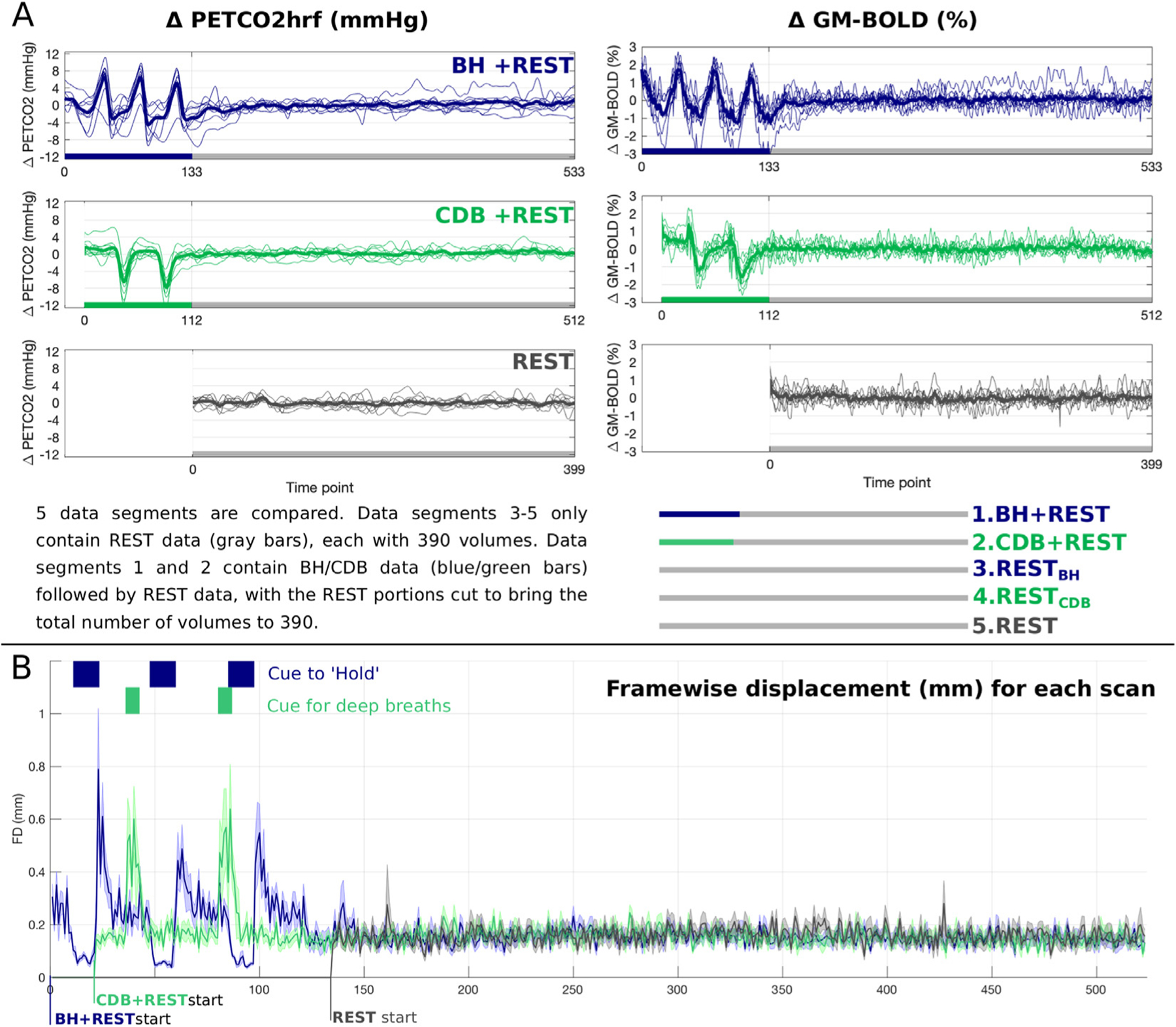
(A) Unshifted P_ET CO₂hrf traces (mmHg change from baseline) and GM-BOLD traces (% change from mean) for each of three fMRI acquisitions. Thick lines represent group means and thin lines represent each subject. The key at the bottom describes the five data segments that are compared in this manuscript. The first 10 volumes at the start of each data segment are not used (discarded to allow steady-state to be reached) resulting in 390 volumes for each data segment. (B) Framewise displacement, created with FSL’s ‘fsl_motion_outliers’ command is plotted for each scan, including blue and green boxes to indicate the time the participant was cued to hold their breath (blue) or take deep breaths (green). The line for each scan represents the mean across subjects and the shading around this line represents the standard deviation. PETCO2 = Partial pressure of End Tidal CO2, hrf = hemodynamic response function, GM = Gray Matter, BOLD = Blood Oxygenation Level Dependent, BH = breath holding, CDB = cued deep breathing.

The hemodynamic lag at each voxel was identified as the shift that gave the maximum full model coefficient of determination (R2 ) (Fig 2-F). If a voxel with an optimal shift (lag) was found at or adjacent to a boundary (−15, −14.6, +14.6, +15) this was not deemed a true optimization and is also less likely to be physiologically plausible (Fig 2-G). Final hemodynamic lag maps (Fig 2-H) display values ranging from negative to positive which indicate earlier to later hemodynamic responses to P_ETCO₂hrf, respectively. Two CVR maps were created: map with no lag optimization (No-Opt), using the unshifted P_ETCO₂hrf as the regressor, and CVR maps with lag optimization (Lag-Opt). Lag-Opt CVR maps used the beta coefficient for the P_ETCO₂hrf regressor from the model with the optimum shift (Fig 2-I). Lag and CVR maps were thresholded (Fig 2-J): CVR values were deemed significant for absolute T-statistics greater than 1.96 (corresponding to p<0.05) and for Lag-Opt CVR this was further adjusted with the Šidák correction (Bright et al., 2017, Sidak, 1967) due to running 101 different models. Voxels with lag values at the boundary were also removed from thresholded parameter maps.

2.2.4. Data summaries and statistical tests

The median GM CVR and the percentage of significant voxels in GM was calculated for each modelled data segment. These values were computed for No-Opt, Lag-Opt, No-Opt with statistical thresholding (p<0.05), Lag-Opt with matched statistical thresholding (p<0.05) and Lag-Opt with stricter statistical thresholding (p<0.05, Šidák corrected). The kernel density estimation of the distribution of lag values in GM (MATLAB’s ksdensity function) was also computed for each subject and each data segment, and the median GM lag values were outputted.

In order to provide lag values with some regional specificity across GM regions, FSL atlases in MNI space (MNI-maxprob-thr25–2mm and HarvardOxford-sub-maxprob-thr25–2mm) were used to make three GM masks: cortical GM, subcortical GM and cerebellar GM. From the HarvardOxford atlas, left and right cerebral cortex parcels were combined into one mask, and left and right subcortical regions (thalamus, caudate, putamen, palladium, hippocampus, amygdala, accumbens) combined into another. The cerebellum parcel was extracted from the MNI atlas to make a third mask. These three atlas masks (cortical, subcortical and cerebellar) were linearly transformed (FSL, FLIRT) to subject space, and thresholded to only include voxels within the subject’s GM tissue mask. Median lag values were extracted from each mask for BH+REST and CDB+REST data segments.

R version 3.4.1 (R Core Team, 2019) was used for data exploration and statistical testing. To compare parameter values across data segments and optimization schemes (No-Opt vs Lag-Opt), repeated measures ANOVAs were run with the R package permuco (Frossard and Renaud, 2019) with the ‘aovperm’ function. Null distributions were created via 100,000 permutations of the original data, which therefore do not depend on gaussian and sphericity assumptions. When investigating simple main effects (‘emmeans’ package) and performing multiple comparisons, p-values were adjusted with the Benjamini & Hochberg approach (Benjamini and Hochberg, 1995) for control of false discovery rate (FDR), and then compared against an alpha of 0.05 to determine significance. Outliers were identified with boxplots. Correlation plots and statistical outputs were created with the R packages ggplot2 (Wickham, 2016) and ggpubr (Kassambara, 2020) with the ‘ggscatter’ function. Outliers for the correlation analysis were identified when Cook’s distance was over 4/n, with n being the number of subjects, which indicates an influential single data point. The Shapiro-Wilk test was used to ensure normality of variables.

It can be seen from the parameter maps (Fig. 5, Fig. 6, Supplementary Figure S1) that after statistical thresholding, a substantial proportion of voxels within white matter do not show a significant relationship between P_ETCO₂hrf and BOLD signals. Therefore, we decided to focus our comparison of CVR and lag parameter averages, across the different data segments, within GM voxels only.

Fig. 5.

Maps of CVR for one example subject (S4). The five main data segments are displayed, as well breathing task only segments (BH only and CBD only) for completeness. No-Opt CVR maps (top row for each data segment) are shown thresholded with the P_ET CO₂hrf regressor at p<0.05. Lag-Opt CVR maps are shown thresholded with the P_ET CO₂hrf regressor at p<0.05 with (middle row) and without (bottom row) Sidak correction, with voxels at lag boundaries removed. BH = breath holding, CDB = cued deep breathing, BOLD = Blood Oxygenation Level Dependent, CVR = Cerebrovascular Reactivity, Opt = Optimization.

Fig. 6.

Maps of hemodynamic lag for one example subject (S4). The five main data segments are displayed, as well breathing task only segments (BH only and CBD only) for completeness. For each data segment, lag maps are shown with no statistical thresholding but voxels at the boundaries removed (top row for each data segment) and shown thresholded with the P_ET CO₂hrf regressor at p<0.05 with (middle row) and without (bottom row) Sidak correction. Values are relative to the GM median. Negative to positive lag values indicate earlier to later BOLD responses to P_ET CO₂hrf. BH = breath holding, CDB = cued deep breathing, GM = Gray Matter.

2.2.5. Resting-state analyses

We performed exploratory analyses to investigate any residual effects on the resting-state data segments that followed the breathing tasks. BOLD-fMRI data from each of the three pre-processed REST segments (7 minutes 48 seconds, first 10 volumes of each segment removed, brain extraction, volume registration) were detrended to remove the same motion parameters and Legendre polynomials as detailed in Sections 2.2.1 and Sections 2.2.3. We then created maps of resting-state fluctuation amplitude normalized to the mean (mRSFA), amplitude of low-frequency fluctuation (ALFF) and fractional ALFF (fALFF) with AFNI’s 3dRSFC function (4 mm FWHM blurring, filtering between 0.01 and 0.1 Hz). We also created maps of local functional connectivity density (LFCD) with AFNI’s 3dLFCD function (Pearson correlation, threshold of 0.6, within a dilated GM mask). Spatial correlations were performed between pairs of single-subject resting-state parameter maps, within the GM mask, with AFNI’s 3ddot function. The resting-state parameter maps were linearly transformed to MNI space and a voxel-wise ANOVA analysis (3dANOVA, AFNI) was run to test the effect of REST segment on mRSFA, ALFF, fALFF and LFCD, setting a voxel-wise threshold of p<0.05 (FDR corrected) for significance.

3. Results

Fig. 3A shows the average BOLD-fMRI signal across GM, and the corresponding P_ETCO₂hrf changes, for each of the three scans. Note the three cycles of increased P_ETCO₂ values in blue, due to breath holds, and the two cycles of decreased P_ETCO₂ values in green, due to cued deep breaths. The fMRI time-series changes as expected due to the CO₂ manipulations. The BH task produced a maximum pressure increase of 7.4±3.1 mmHg (mean±stdev across subjects) and CDB produced a maximum decrease of 8.1±3.2 mmHg, relative to the mean value at rest. For the three rest segments the temporal standard deviation of P_ETCO₂ was 0.9±0.4, 1.2±0.7 and 0.8±0.4 mmHg (mean±stdev across subjects) for REST, REST_BH and REST_CDB respectively. Fig. 3B displays framewise displacement (Power et al., 2012) to summarize head motion, showing increased motion during breathing tasks.

3.1. Hemodynamic lag values

Fig. 4 shows the distribution of hemodynamic lag values in GM tissue estimated from the lagged-GLM analysis, displaying both positive and negative lags. Though a positive lag value might be expected (CO₂ pressure change in the blood leads the fMRI signal change) there are multiple factors contributing to this value, and in different directions. For example, the recording delay between CO₂ exhalation inside the scanner and CO₂ recording outside the scanner contributes to a more negative shift, whereas vascular transit delays and vasodilatory dynamics that eventually lead to the BOLD-fMRI signal will contribute to a more positive shift. Therefore, the observed lag between a CO₂ recording and a BOLD fMRI recording will naturally vary with the experimental set-up, the participant, and their physiological state.

Fig. 4.

Distributions of lag values, across GM voxels. Distributions for all subjects (S1-S9) are shown, and for all data segments. Negative to positive lag values indicate earlier to later BOLD responses to P_ET CO₂hrf. The percentage (per) of GM voxels with optimal shift values at the boundary condition is compared across data segments in the bottom right-hand corner. The group mean is shown as a thick horizontal line and each subject is represented as a black dot. Lag values are not relative to GM median. BH = breath holding, CDB = cued deep breathing, GM = Gray Matter, pde = probability density estimate.

As demonstrated in Fig. 4, the BH+REST and CDB+REST data segments, plotted in solid blue and green lines respectively, have a more gaussian-like distribution of lag values (excluding the boundaries), the properties of which generally match for most subjects. REST data segments (dashed lines) have less physiologically plausible distributions which agree less with other segments and vary more across subjects. Fig. 4 also shows the percentage of GM voxels with lag values at the boundary condition. From the repeated measures ANOVA analysis, there was a significant effect of data segment on percentage of voxels at the boundary condition (F(4,32) = 9.86, p < 0.0001). Simple main effects analysis showed that group means for BH+REST (12.24%) and CDB+REST (11.79%) did not differ (p=0.795, FDR-corrected). However, BH+REST and CDB+REST each had a significantly lower percentage compared to REST (17.56%), REST_BH (17.35%) and REST_CDB (18.34%), with all p-values < 0.022, FDR corrected. All REST segment pairs were not significantly different to each other (p>0.605, FDR corrected). This analysis was run multiple times after the separate removal of three data points from the REST_CDB group which were classed as extreme outliers based on boxplots, however the results did not change. The three REST data segments resulted in a greater percentage of voxels being identified at the boundaries of our fitting procedure; lag values at the boundary are less physiologically plausible, and indicate less certain lag optimization i.e., we cannot determine this is a true local maximum.

Supplementary Table S1 shows that BOLD response timing to a P_ETCO₂hrf change is generally earliest in subcortical GM regions, approximately 0.4 seconds later in cortical GM regions, and 1.4–2.0 seconds later in GM cerebellar regions. Though specific regional comparisons were not a focus of this paper, lag (CVR delay) is less commonly characterized in the literature, compared to CVR amplitude. Therefore, these results are included in order to assess the agreement of our lag values with previous literature.

3.2. CVR and lag maps

Figs. 5 and 6 show maps of CVR and lag, respectively, for one subject and all thresholding options. CVR values increase after lag optimization, as expected. There is more spatial agreement in CVR and lag maps when the BH and CDB segments are included in the modelled data, showing a similar contrast between tissues types. Maps that only include REST data barely exhibit a physiologically reasonable contrast between tissues types, and after the final statistical thresholding (p<0.05, Šidák corrected) very few voxels remain. This is also seen in Supplementary Figure S1, which displays maps for all subjects. All subjects follow the trend described, except S7 and S8 which have CDB+REST maps that appear more similar to REST maps (in number and distribution of significant voxels); these are the same two subjects in Fig. 4 that had CDB+REST GM lag distributions that did not look similar to the BH+REST distributions.

3.3. Comparing GM CVR values and significant fits across data segments

Fig. 7 depicts the distribution of CVR values in GM, for No-Opt CVR and Lag-Opt CVR across different levels of statistical thresholding, for one subject. The same plots can be found for all subjects in Supplementary Figures S2-S6. In general, the No-Opt CVR values (row 1) follow a Gaussian- or Laplacian-like distribution when no statistical thresholding is applied. The REST data segments generally have the greatest number of negative CVR values. The Lag-Opt CVR distributions (unthresholded, row 2) change shape to resemble a more bimodal distribution, due to CVR estimates diverging further from zero in either direction (which is expected due to our method for optimizing lag). This effect is enhanced in the thresholded distributions for both No-Opt and Lag-Opt (rows 3–5); CVR values closer to zero are removed after applying statistical criteria, resulting in distinct bimodal distributions. Interestingly, we see the proportion of negative CVR values to positive CVR values is much less in the BH+REST and CDB+REST data segments. For the REST segments, after lag optimization and statistically thresholding there are some cases where there is an equivalent amount of positive and negative CVR values. We expect predominantly positive CVR values in GM, and true negative CVR responses represent very different physiological mechanisms (Thomas et al., 2013, Bright et al., 2014). Considering the shape of these distributions, and the considerable proportion of negative CVR values in the REST segments, we summarized positive and negative CVR separately when computing summary CVR metrics across GM, shown in Fig. 8 and Supplementary Figure S7. For ease of reference, group averages and standard deviations from these figures are also provided in Supplementary Table S2.

Fig. 7.

Distributions of CVR values in GM for one example subject (S4). The y-axes show the frequency count. The same scaling is used for rows 1 and 2 because no thresholding is applied and therefore all GM voxels are included. When statistical thresholding is applied (rows 3, 4 and 5), different numbers of GM voxels remain for each data segment. BH = breath holding, CDB = cued deep breathing, GM = Gray Matter, BOLD = Blood Oxygenation Level Dependent, CVR = Cerebrovascular Reactivity, Opt = Optimization.

Fig. 8.

Comparing GM summary metrics across the five data segments. Top: Median positive CVR across all GM voxels for No-Opt and Lag-Opt analyses. Bottom: Percentage of significant positive fits in GM for each data segment and level of thresholding: the [∗ ] indicates thresholding at p<0.05 and [∗ (s)] indicates thresholding at p<0.05 with Sidak correction. BH = breath holding, CDB = cued deep breathing, GM = Gray Matter, BOLD = Blood Oxygenation Level Dependent, CVR = Cerebrovascular Reactivity, Opt = Optimization.

Fig. 8 (top panel) compares median positive GM CVR values across data segments. There was a significant interaction between data segment and optimization scheme (F(4,32 = 14.2, p<0.00001) so simple effects were investigated. Positive GM CVR values increased after lag optimization for all data segments: BH+REST (p=0.02), CDB+REST (p=0.01), REST (p=0.002), REST_BH (p=0.002) and REST_CDB (p=0.002). There were no significant differences in median positive GM CVR values between any pair of data segments for No-Opt values (all p-values >0.14) but there were significant differences for Lag-Opt values, which drove the significant interaction. For Lag-Opt, positive GM CVR values were not different between: BH+REST and CDB+REST; CDB+REST and REST; CDB+REST and REST_BH; REST and REST_BH (all p-values >0.14), However, REST had significantly higher values than BH+REST (p=0.02); REST_BH had significantly higher values than BH+REST (p=0.006); REST_CDB had significantly higher values than BH+REST (p=0.001), CDB+REST (p=0.001), REST (p=0.002), and REST_BH (p=0.008). One extreme outlier was removed from the CDB+REST segment (Fig. 8, subject with highest values) for this statistical testing. All p-values are FDR corrected. Similar patterns are seen for negative CVR values (Supplementary Figure S7).

The previous CVR comparisons are taken using all GM voxels, and not only from voxels that are statistically thresholded; Fig. 8 (bottom panel) shows that the percentage of significant voxels in GM is noticeably lower in the REST data segments, suggesting that there is less confidence in these summary CVR estimates. With or without lag optimization, there are more GM voxels showing significant positive fits for P_ETCO₂hrf in the data segments with breathing tasks, for all subjects except S7 and S8. The inverted V-shaped pattern shows the number of significant voxels changes with statistical thresholding in a similar way across the 5 data segments: more voxels are significant after lag optimization if the same thresholding (p<0.05) is applied, however after Šidák correction this returns to a similar or smaller number of statistically significant voxels as found without lag optimization. This shows the statistical consequence of the lagged-GLM computation (considered further in the discussion).

3.4. Clinical utility

An incidental finding was suspected in one of our participants due to an abnormality first noticed in the lag maps. Specifically, a large section of the cortex displayed a blood flow response to P_ETCO₂ much later than other areas of the cortex. The area of cortex impacted appeared to be the vascular territory mostly supplied by the middle cerebral artery. The appropriate ethical procedures were followed and it was confirmed that this subject had unilateral Moyamoya disease. Moyamoya is a rare vascular disorder which typically involves blockage or narrowing of the carotid artery, reducing blood flow to the brain. Fig. 9 shows CVR and lag maps in this subject. The lag maps show that many GM voxels in the right hemisphere are responding approximately 10 seconds later compared to the homologous regions of the left hemisphere. When lag is not considered, the CVR maps (No-Opt) show dominant negative CVR in this vascular territory, similar to what has been reported in previous CVR mapping studies with Moyamoya (Conklin et al., 2010, Poublanc et al., 2013, Dlamini et al., 2018). However, when correcting the CVR maps for lag (Lag-Opt) there is a striking change - the CVR within GM mostly normalizes, without a clear pathology. These lag-optimized maps suggest that the local CVR response is preserved in GM, albeit with delayed blood transits. Looking at the lag optimized CVR map alone, one could incorrectly conclude that this subject does not have a clear vascular pathology. Both maps, lag and CVR (Lag-Opt), are needed for the most accurate interpretation, and to determine whether there are CVR reductions, delayed blood transits, or both. Fig. 9 also shows CVR and lag results in REST data. Here, the pathology is much less evident, and these results follow the same pattern seen in the other 9 subjects presented.

Fig. 9.

Maps of lag and CVR for a subject with Moyamoya disease. The white box shows results for the BH+REST data, demonstrating clear clinical sensitivity of this protocol. In order to visually compare maps across the same voxels, all maps (CVR No-Opt, CVR Lag-Opt and Lag) are thresholded at p<0.05, Sidak corrected, based on the T statistics of the lag optimized analysis. The REST only results are shown for comparison at p < 0.05 uncorrected as well as the p<0.05 Sidak corrected which displays very few significant voxels. Slices from the T1-weighted image transformed to fMRI space are shown for reference. CVR Lag-Opt maps, and all lag maps, do not include voxels with lags found at the boundary. Lag maps are not relative to GM median but the analysis for this subject is run the same was as previously presented for the 9 other subjects. Negative to positive lag values indicate earlier to later BOLD responses to P_ET CO₂hrf. BH = breath holding, BOLD = Blood Oxygenation Level Dependent, CVR = Cerebrovascular Reactivity, Opt = Optimization.

In a concurrent pediatric pilot study, five individuals with typical development and hemiparetic cerebral palsy completed a modified version of the CDB+REST protocol. Fig. 10 shows P_ETCO₂ traces and average BOLD-fMRI signal across GM. Three primary scenarios of task compliance were observed. In Scenario 1, participants achieved hypocapnia as expected, evidenced by two consecutive decreases in P_ETCO₂ and BOLD-fMRI signals. In Scenario 2, P_ETCO₂ values were unreliable for several breathing cycles (indicated by missing values in Fig. 10), yet there is possible evidence of two mild hypocapnia cycles in the BOLD-fMRI signal. In Scenario 3, P_ETCO₂ values were more reliable but participants did not appear to complete the task, evidenced by a lack of hypocapnia-induced P_ETCO₂ and BOLD signal decreases. These trends appear to be age-related, with scenario 1 primarily occurring in older participants (ages 15–21 years) and scenarios 2 and 3 in the youngest participants (7–12 years).

3.5. Resting-state analyses

For all resting-state metrics, no significant differences were found between resting data segments, and therefore no clear evidence of residual effects caused by breathing tasks were identified. For mRSFA, group means ± stdev for spatial correlations between pairs of single-subject maps were: 0.92±0.04 (REST, REST_BH), 0.92±0.06 (REST, REST_CDB) and 0.92±0.04 (REST_BH, REST_CDB). For ALFF: 0.92±0.04 (REST, REST_BH), 0.93±0.04 (REST, REST_CDB) and 0.93±0.03 (REST_BH, REST_CDB). For fALFF: 0.87±0.08 (REST, REST_BH), 0.91±0.03 (REST, REST_CDB), 0.90±0.05 (REST_BH, REST_CDB). For LFCD: 0.62±0.21 (REST, REST_BH), 0.58±0.25 (REST, REST_CDB), 0.66±0.19 (REST_BH, REST_CDB). For the voxel-wise ANOVA, we observed no voxels with a significant (p<0.05, FDR corrected) main effect or significant pairwise comparison for mRSFA, ALFF, fALFF or LFCD parameter maps. The lowest FDR corrected p-value across all pairwise comparisons and parameter maps was 0.51.

4. Discussion

Adding a simple, 2–3-minute breathing task to the beginning of a resting-state scan vastly improves our ability to model CO₂ effects (both amplitude and timing) in BOLD-fMRI data. This modified scan protocol produces maps of physiological parameters that may contribute to our understanding of healthy and pathological cerebrovascular function, whilst maintaining an extended “resting state” period as required for studying intrinsic brain fluctuations and connectivity. This hybrid protocol has clear and direct applications for CVR mapping in both research and clinical settings, as well as wider applications for fMRI denoising and interpretation. Our analysis produces maps of both the amplitude (CVR) and timing (hemodynamic lag) of the BOLD fMRI response to CO₂ by systematically shifting the P_ETCO₂ regressor to optimize the model fit. In any fMRI dataset, this optimization inherently increases GM CVR values and fit statistics. We have shown that the inclusion of breathing task data further increases the number of voxels in the brain that have a significant relationship between P_ETCO₂ and BOLD-fMRI signals, and improves our confidence in the plausibility of voxel-wise hemodynamic lag estimates.

Compared to a typical resting-state fMRI scan, this protocol requires extra equipment to record expired CO₂ alongside scanner triggers. For the benefits gained, this cost is reasonable relative to typical scanning costs, and the equipment is easy to set-up and maintain. In our experience, healthy pediatric and adult cohorts find wearing the nasal cannula comfortable throughout the scanning session. It is important to acknowledge that previous studies have successfully mapped CVR with-out normalizing the BOLD change by the P_ETCO₂ change, for example, by using an average BOLD time course in replace of a P_ETCO₂ regressor (Liu et al., 2017) or using metrics such as RSFA or ALFF (Golestani et al., 2016) as representations of CVR function. For some applications, qualitative CVR metrics may be sufficient; however, we chose to normalize BOLD change by the P_ETCO₂ change to allow more direct comparisons with other literature and to take in account task compliance differences (discussed further in (Pinto et al., 2021)).

A recent study (Liu et al., 2020) followed a very similar rationale to ours: to develop a practical non-gas inhalation method that is largely based in a resting-state scan but introduces breathing modulations to enhance fluctuations in P_ETCO₂. They compared CVR maps from resting-state scans, scans with intermittent breathing modulations throughout the scan period (for a duration of 12 seconds after 30–60 s of free breathing), a breath-holding scan, and a CO₂ gas inhalation scan. They showed that intermittent breathing modulations (6 seconds per breath) had a comfort level similar to resting-state, and the resultant CVR maps had a sensitivity and accuracy similar to maps derived from gas inhalation methods. Hemodynamic lag was not a part of their assessment or comparisons. Their results are consistent with our conclusions that adding short periods of guided breathing is favorable over a resting-state scan for CVR mapping, and they have validated their design by comparing to a more gold standard CO₂-inhalation approach. However, their breathing task and resting-state portion cannot be separated into two sections, precluding these data from being used for typical resting-state or functional connectivity analyses.

One reason that including breathing tasks benefits CVR mapping is simply that the induced variation in P_ETCO₂ amplitude is large compared to the smaller fluctuations during undirected free breathing (see Fig. 3A). Importantly, the amplitude of these natural fluctuations during resting-state will vary across subjects, and potentially across study populations (Lynch et al., 2020). If the BOLD fluctuations related to P_ETCO₂ changes are small in amplitude, it can be hard to distinguish them from other physiological, artefactual or neuronally-driven fluctuations that occur at (or aliased into) the same low-frequencies (Murphy et al., 2013, Liu, 2016, Caballero-Gaudes and Reynolds, 2017, Tong et al., 2019, Whittaker et al., 2019). If these other fluctuations are of similar or greater magnitude to the low-frequency fluctuations induced by P_ETCO₂, this may result in an fMRI time-course poorly coupled to P_ETCO₂. A study using gas inhalation as a hypercapnic stimulus concluded that a change of at least 2 mmHg above a subject’s baseline P_ETCO₂ is necessary to evaluate hemodynamic impairment (De Vis et al., 2018). In our acquisitions, both BH and CDB tasks clearly produced changes above 2 mmHg, whereas this was not the case for all subjects during the REST segments (see Fig. 3A). Even if a subject performs the BH or CDB task only partially (i.e., shorter hold for the BH, shallower breaths for the CDB), they are likely to still surpass this 2 mmHg change. Furthermore, there is evidence that despite variability in BH performance, robust and repeatable CVR maps can still be obtained when modeling with P_ETCO₂ regressor (Moia et al., 2021, Bright and Murphy, 2013), which represents what the subject actually achieved and not simply the intended stimulus.

To accurately model CVR we must account for hemodynamic lags since measurement delays in gas sampling, arterial transit times to the brain’s vascular territories, and local vasodilatory dynamics all impact the temporal relationship between our model of the vasodilatory stimulus (P_ETCO₂) and the BOLD fMRI timeseries. Characterizing hemodynamic lag at the voxel level is both challenging and necessary for correct physiologic interpretation of the data. A previous study mapping CVR with resting-state data discussed how they were unable to obtain voxel-wise delays due to the resultant CVR maps being noisy, and they acknowledge that the regional CVR deficits they report in Moyamoya patients may reflect both reduced CVR and longer blood transits (Liu et al., 2017). We report similar challenges in our data (Fig. 4, Fig. 6, Supp. Figure 1), showing more variable and less physiologically plausible lag distributions across GM in the data modelled with only resting-state segments. Furthermore, when simply performing a cross-correlation between the P_ETCO₂hrf regressor and GM BOLD-fMRI time-series, we observe several extreme lag values in resting-state data (see Appendix A). The incorporation of the short breathing tasks results in more sensible lag distributions and cross-correlation results. Comparing our lag values to previous literature is challenging due to the multitude of experimental set-ups, analysis approaches, and ways of summarizing these types of data. Nevertheless, it is valid to compare normalized lag values (lag values relative to a tissue average) and compare variability in lag, where possible. Here, we focus on BH+REST and CDB+REST lag distributions, considering REST distributions are challenging to summarize (Fig. 4). The range and variability of the lag values we report in GM show the majority of lag values (~68% based on one standard deviation, Supp. Table 1) are within 6 seconds of the GM median (Fig. 6, Supplementary Figure S1); therefore, to capture the majority of GM lags a range of 12 seconds from the GM median may be appropriate. This broadly agrees with previous work using respiration derived or P_ETCO₂ regressors (Chang and Glover, 2009, Bright et al., 2009, Birn et al., 2008, Sousa et al., 2014, Donahue et al., 2016, Moia et al., 2020, Moia et al., 2021). Many of these previous reports also see similar regional trends in relative lag values (Supplementary Table S1): earliest responses in subcortical GM and later responses in cerebellar GM and posterior brain regions.

Despite much previous literature reporting a summary CVR value, our results clearly show that analysis choices in summarizing voxel-wise CVR values are not trivial. The distributions of GM CVR values with and without lag optimization, and with different levels of statistical thresholding (Fig. 7, Sup. Figures S2-S6), illustrate that it is not strictly valid to extract a central tendency value from a distribution of positive and negative CVR values together, after lag optimization or any statistical thresholding. We therefore chose to summarize positive and negative CVR values separately, not least because true negative CVR responses represent very different physiological mechanisms (Thomas et al., 2013, Bright et al., 2014). We expect positive CVR values in GM, and it is noteworthy that the three resting-state segments show a greater number of negative CVR values compared to the segments that include BH or CDB tasks, possibly suggesting a greater relative contribution of noise sources and a less successful CVR and lag estimation. The final summative CVR value across a tissue type will also depend on whether one has applied lag optimization and/or applied statistical thresholding. Therefore, we chose to display CVR values resulting from multiple analysis options in Fig. 8 and Supplementary Figure S7. With no statistical thresholding, the positive GM CVR amplitudes for No-Opt and Lag-Opt (Fig. 8 and Supplementary Table S2) agree with the range seen in previous literature modeling CVR with breathing tasks or resting-state, when expressed in units of %BOLD/mmHg (Liu et al., 2020, Lipp et al., 2015, Pinto et al., 2016, Sousa et al., 2014, Moia et al., 2020, Bright and Murphy, 2013, Bright et al., 2011). Unexpectedly, the REST segments showed higher GM CVR values than the task segments after lag optimization and following the strictest thresholding, particularly for REST_CDB (Fig. 8, Supplementary Figure S7). However, a higher CVR value will not always suggest a more accurate or more representative tissue estimate. Low frequency fluctuations other than P_ETCO_2, motion artifacts and large vessel signals may influence the lagged fitting procedure, as discussed. There were generally more negative CVR values in REST segments, so positive GM CVR estimates are also summarized over a smaller number of voxels that do not fully describe GM tissue. It is also important to note that the Sidák correction is likely too strict of a correction for multiple comparisons as it assumes independence, which is not the case when running the GLM multiples times with slightly shifted P_ETCO₂ regressors.

4.1. Choice of breathing task

This study was not designed for an effective comparison between BH or CDB, yet some trends can be noted upon. Adding either a short BH or CDB task to a resting segment brings clear advantages for CVR mapping, with similar CVR and lag results. Direct comparison of these two tasks is potentially biased due to the BH task being slightly longer, including 3 cycles of hypercapnia versus 2 cycles of hypocapnia for the CDB task. It is difficult to match both the length of the breathing task, and the number of cycles: the ways in which we achieve hypocapnia (increasing the rate and depth of breathing) and hypercapnia (apnea) are very different, and the timing dynamics of the resulting blood gas changes can be different, particularly in sustained challenges (Kasprowicz et al., 2012, Poulin et al., 1996, Poulin et al., 1998). A small amount of previous evidence shows that more transient CO₂ modulations induced by CDB and BH tasks generally lead to comparable CVR amplitudes and timings (Bright et al., 2009), however possibly not in all brain regions (Bright et al., 2011) and they can be modulated differently by baseline vasodilation (Bright et al., 2011). Furthermore, these tasks induce different motion confounds (Bright et al., 2009) (Fig. 3B) and potentially different subject compliance demands. In general, our results suggest that these tasks may be used interchangeably in healthy controls. However, we recommend BH because it leads to plausible lag distributions and significant CVR effects more consistently, and there is more extensive literature using this task for CVR mapping (Urback et al., 2017, Pinto et al., 2021). Importantly, vasoconstrictive and vasodilatory responses can be differentially affected in pathology (Zhao et al., 2009) and therefore different tasks may be appropriate for different clinical populations and research questions. Furthermore, while all subjects in this study were able to adequately perform both breathing tasks, pediatric, elderly or clinical cohorts may comply better with the CDB task considering the simplicity of instructions. A more thorough comparison of the pros and cons of these breathing tasks, in larger healthy and clinical cohorts, is a worthwhile focus for future research.

It is important to discuss the general limitations of using breathing tasks to model CVR, compared to resting-state. They do require more compliance from subjects, introduce neural activity due to the need for visual or auditory stimuli, and often exhibit motion effects correlated with task timings (Fig. 3B) (Bright et al., 2009, Power et al., 2018, Power et al., 2017, Moia et al., 2021). We performed volume realignment and included the resultant motion parameters within the GLM, but there is evidence this is not sufficient to remove motion effects (Power et al., 2017, Moia et al., 2021, Power et al., 2014). Further research should look into optimizing breathing task designs to minimize task induced motion artifacts whilst still maintaining P_ETCO₂ changes of sufficient amplitude. Collecting multi-echo BOLD fMRI data, and applying spatial ICA-denoising analyses, is one widely adopted strategy that can be applied to remove motion artifacts and has been applied to the modeling of CVR effects in BH paradigms (Cohen and Wang, 2019, Moia et al., 2021). A final consideration is the choice of HRF in breathing task data; here we used a canonical HRF to convolve with all the P_ETCO₂ time-series, before creating the multiple shifted P_ETCO₂ regressors. There is evidence that the BOLD signal may have a different shape and timing response depending on whether the P_ETCO₂ is resting fluctuations, or within a hypocapnic or hypercapnic range and that physiological response functions can vary across subjects, brain regions and sessions (Chang and Glover, 2009, Birn et al., 2008, Kassinopoulos and Mitsis, 2019, Golestani et al., 2015). By shifting the P_ETCO₂hrf in time with the lagged-GLM approach, variation in latency will be well accounted for but not variation in the shape of the response. Therefore, it is likely that a single response function will not be optimum for capturing all the P_ETCO₂ induced BOLD changes during rest, deep breaths and breath-holds, a potential limitation when modeling these segments together.

4.2. Clinical applications

We chose to analyze and present our results in single subject space, partially to demonstrate the potential utility of this method for individual subjects, such as clinical cases, or individual fMRI denoising. We report an incidental finding of unilateral Moyamoya disease, which was first identified during inspection of the hemodynamic lag maps constructed from our lagged-GLM approach. This pathology was only visually obvious when modeling lag and CVR with breathing task data. Regional deficits in CVR are used to guide surgical and treatment decisions in cases of Moyamoya (Bacigaluppi et al., 2009), with normalization of CVR often seen after surgery. Delayed blood transits are also widely reported in cases of Moyamoya (Donahue et al., 2016, Poublanc et al., 2013, Schubert et al., 2009) which is expected due to the narrowing of blood vessels. Consistent with our non-optimized results, negative CVR responses are often observed in cases of Moyamoya (Conklin et al., 2010, Poublanc et al., 2013, Dlamini et al., 2018) and commonly interpreted as the vascular steal phenomenon. In the case of vascular steal, negative CVR is the result of a redistribution of blood flow from regions without remaining cerebrovascular reserve to regions with preserved vasodilatory capacity. Previous work with cases of Moyamoya have shown a clear relationship between blood arrival times and CVR amplitudes, with the longest arrival times having the lowest and most negative CVR (e.g., (Poublanc et al., 2013, Schubert et al., 2009). In our data, it is possible to conclude there is no evidence of vascular steal, considering the normalization of CVR after lag-optimization, however other work suggests that negative CVR is likely a combination of a steal phenomenon and delayed local (positive) reactivity (Poublanc et al., 2013). We would need to apply our technique more systematically across a larger sample to better characterize these subtleties of Moyamoya pathology, yet what our case study clearly demonstrates is the importance of considering both amplitude and timing when modeling CVR function in pathology. CVR deficits in Moyamoya are most commonly investigated with gas inhalation or contrast; although there is a much smaller collection of literature using breath-hold or resting-state, the interest in these non-invasive and practical approaches is growing (Taneja et al., 2019, Donahue et al., 2016, Dlamini et al., 2018, Liu et al., 2017, Christen et al., 2015).

Example data from a separate pediatric pilot study were included to evaluate the feasibility of our hybrid protocol in clinical cohorts with task compliance challenges (e.g., children). Breathing tasks are an attractive alternative to more invasive vasoactive stimuli; BH tasks have been used successfully in typically developing children (Thomason et al., 2005) and in those with Moyamoya (Dlamini et al., 2018). We report the first instance of a CDB task in a pediatric cohort and observed variable success in the quality of P_ETCO₂ recordings and achieved hypocapnia. These results indicate that further optimization of the breathing task portion of the hybrid design may be necessary in less-compliant cohorts. Low quality P_ETCO₂ traces may be caused by periods of mouth breathing and could be addressed by using a mask rather than a nasal cannula. It may be necessary to adapt breathing task instructions for clarity and utilize practice sessions, tailored to the population, to ensure participants understand and comply with the task before entering the scanner. There are clear next steps to address the feasibility limitations observed in our hybrid design and, once these are met, this method has promise as a practical yet robust tool to study typical and atypical neurovascular development.

4.3. Why should we append breathing tasks to the start of a resting-state scan instead of keeping them separate?

Based on the mechanism of neurovascular coupling, the BOLD contrast is widely used as a surrogate measure for neural activity (Glover, 2011). However, there are many non-neural factors that can affect the BOLD signal, with multiple strategies and algorithms to mitigate and remove these sources of noise, (Wise et al., 2004, Murphy et al., 2013, Caballero-Gaudes and Reynolds, 2017, Greve et al., 2013, Bright and Murphy, 2017, Liu, 2013, Chu et al., 2018, Kim and Ogawa, 2012). We considered how resting-state fMRI scans are commonly deployed in neuroimaging research, and designed our protocol accordingly. Although the main focus of the work presented here is practical CVR mapping, CO₂ fluctuations have been shown to be a physiological confound in resting-state fMRI studies of neural activity, and it is challenging to meaningfully separate out neural connectivity and vascular connectivity with fMRI data (Power et al., 2018, Chu et al., 2018, Madjar et al., 2012, Nikolaou et al., 2015, Bright et al., 2020, Chen et al., 2020). Removing CO₂ effects from fMRI via nuisance regression is not yet routine practice, in part because it is challenging to robustly characterize these relationships in resting-state fMRI.

The main benefit of using overlapping data for multiple analyses (e.g., CVR and resting-state analyses) is that it saves both scanning time and analysis time (e.g., some of the same pre-processing steps and creation of physiological regressors can be used for both analyses). By appending a short breathing task to the start of a resting-state scan, the resting-state portion could still be analyzed separately, gaining more outputs from one dataset, with improved denoising from robust modeling of CO₂ effects. However, two key questions arise when considering the use of overlapping data: (1) are there residual effects from the breathing tasks that would systematically affect the resting-state portions that follow (similar to after effects seen after other sensory and cognitive tasks (Tung et al., 2013, Gaviria et al., 2020))? and (2) is modeling of CVR worse by including the resting portion alongside the breathing task portion?

Related to (1), our exploratory resting-state analyses showed no clear systematic differences between the three REST segments (two with breathing tasks preceding, one without) for mRSFA, ALFF, fALFF or LFCD outputs, after minimal preprocessing and denoising. However, these analyses cannot provide direct evidence for the null hypothesis, and future work with study designs tailored towards this question should investigate this further. If a researcher is concerned about residual effects, they could put the breathing task after the resting-state portion and not before; we chose to put the breathing task at the start to ensure the participant was most alert. Another option is to keep the scans separate to avoid any interaction between these two data segments, but then other benefits will be lost.

Related to (2), we ran the lagged-GLM with breathing task data only, without the rest portion (Figs. 5 and 6, Supplementary Figure S8, Supplementary Table S3). We found more significant CVR effects when modeling with more data points (greater degrees of freedom in model fit) and no indication of worse lag or CVR estimation when rest portions are included. These results suggest that CVR and lag can be adequately modelled with only 2–3 minutes of breathing task data, particularly in the case of BH.

4.4. Recommendations and practical considerations

The proposed protocol will not be the best approach for all CVR mapping experiments; if CVR is your primary research focus, longer breathing tasks or gas inhalation methods in a dedicated scan are recommended. Our protocol aims to be a practical addition to the commonly collected resting-state fMRI scan, as well as being a clinically feasible approach to mapping CVR and lag in situations where more invasive or complicated methods are less desirable. In these studies, we make the following recommendations.

• Collect continuous CO₂ recordings before and after your scan window, up to the maximum shift you want to consider in your modeling, to avoid extrapolation or trimming of data after shifting.

• If deciding between a BH or CDB task, we currently recommend BH when studying healthy cohorts.

• If using the BH+REST or CDB+REST design as shown in Fig. 1, model CVR using the entire dataset. In this paper, we cut the TASK+REST segment to 8 minutes in order to make a fair comparison with the 8–minute REST segments. Therefore, our CVR and lag maps are from modeling with ~2.5 minutes of task data and 5.5 minutes of resting data; map quality and fit statistics would likely improve with more data.

• Use the smallest range of shifted P_ETCO₂ regressors as is appropriate for the physiology of your cohort. There are computational and statistical consequences to extending the shift range more than is necessary.

• If there is a large offset between the P_ETCO₂ trace and the GM fMRI signal, perhaps due to a measurement delay (e.g., long sample line from scanner to control room), consider first performing a bulk-shift (cross-correlation between a mean GM fMRI time-series and P_ETCO₂ time-series) before voxel-wise optimization (see Appendix A).

• When obtaining a summary CVR or lag metric for a tissue class, check the distributions to see if this is valid and appropriate; consider whether you need to characterize positive and negative CVR separately.

5. Conclusions

We have demonstrated that adding a short breathing task to the start of a resting-state fMRI scan improves the ability to model both the timing and amplitude of the CVR response, both crucially important for the accurate characterization of cerebrovascular function. This hybrid protocol has direct applications for CVR mapping in both research and clinical settings and wider applications for fMRI denoising and interpretation.

Abbreviations:

No-Opt

No Optimization

Lag-Opt

Lag Optimization

HRF/hrf

Hemodynamic Response Function

PaCO₂

Partial pressure arterial CO₂

P_ET CO₂

Partial pressure of End Tidal CO₂

BH

Breath Holding

CDB

Cued Deep Breathing

GLM

Generalized Linear Model

SBRef

Single Band Reference image

GM

Gray matter

CVR

Cerebrovascular reactivity

Appendix A. Further details on creating shifted P_ETCO₂hrf regressors

The choice of the shift range (15 seconds before & after the reference start time) and the shift unit (0.3 seconds), explained in Fig. 2, was not the focus of this study. However, this topic warrants further justification and explanation.

Shift range: Searching in a range of ±9 s (around an average value) for the optimum P_ETCO₂ shift is consistent with research in healthy subjects which report lag values from modeling with breathing task regressors (Chang et al., 2008, Chang and Glover, 2009, Bright et al., 2009, Birn et al., 2008, Sousa et al., 2014, Tong et al., 2014, Donahue et al., 2016, Blockley et al., 2011). It is not always clear if it is valid to interpret lag values from previous studies as absolute or relative, and what they are relative to, due to differences in data acquisition, data analysis and the cohort studied. Therefore, in our previous work using breath-hold data only (Moia et al., 2020, Moia et al., 2021) we also performed an initial gross realignment (a “bulk shift”) before creating the multiple P_ETCO₂hrf regressors which are shifted at the finer resolution, consisting of a cross-correlation between an average GM BOLD time-series and the original unshifted P_ETCO₂ time-series. Performing a bulk shift in this way is likely to largely account for variation in measurement delays. However, global physiological delays may still contribute due to the way this bulk shift is estimated. Future work using such methods should attempt to separate out measurement contributions (e.g., delays through the cannula and tubes) from physiological contributions. The advantage of performing a bulk shift is that fewer shifted models need to be run in order to characterize the physiological range of voxel-wise lags, therefore reducing computation and making the Šidák corrected alpha value for statistical significance less stringent.

In this current work, no bulk shift was performed due to finding physiologically implausible optimum bulk shift values for the REST only segments (e.g., 19 and 20 seconds at the most extreme, see Fig. A1, y-axis), which could introduce substantial timing errors near the start of the analysis protocol that would propagate to the final parameter maps. We hypothesize that this could be due to the intrinsic low-frequency oscillations associated with neural activity that can be of similar or greater magnitude to the low-frequency fluctuations induced by P_ETCO₂, resulting in a GM fMRI time-course poorly coupled to P_ETCO₂. Motion and other physiological noise could also contribute. Therefore, instead of applying a bulk shift, we chose to apply our voxel-wise lag optimization method with a larger shift range, searching within ±15 s from the reference start time. This 15 second range was based on a 9 second range plus the largest bulk shift seen across subjects for the BH+REST and CDB+REST data segments, which was −5.45 seconds. Fig. A.1 also shows how well this bulk shift agreed with the GM median lag from the voxel-wise lagged-GLM analysis, two different methods of characterizing a representative GM lag value. Data segments with breathing tasks show the strongest significant positive correlations. The REST_BH and REST_CDB segments also show strong significant positive correlations, though with more extreme values for the cross-correlation method. The REST segment did not show a significant correlation between methods. These results indicate that there is clear consistency between different methods of summarizing a GM lag value when including either breathing task; this consistency is present in some, but not all, REST segments.

Shift unit: The true CVR response time (lag) will not be physiologically constrained to the sampling rate of the fMRI scan or of the breathing rate. Despite only sampling end-tidal CO₂ pressure at the end of each breath, a linear interpolation between these values is performed to give an estimate of how the pressure of arterial CO₂ is likely to be changing at a finer temporal scale. Therefore, we chose to shift the high resolution P_ETCO₂hrf time-series at 0.3 seconds (4 times the resolution of the imaging TR) to reflect this, although more validation for the choice of this shift unit is needed.

Fig. A1.

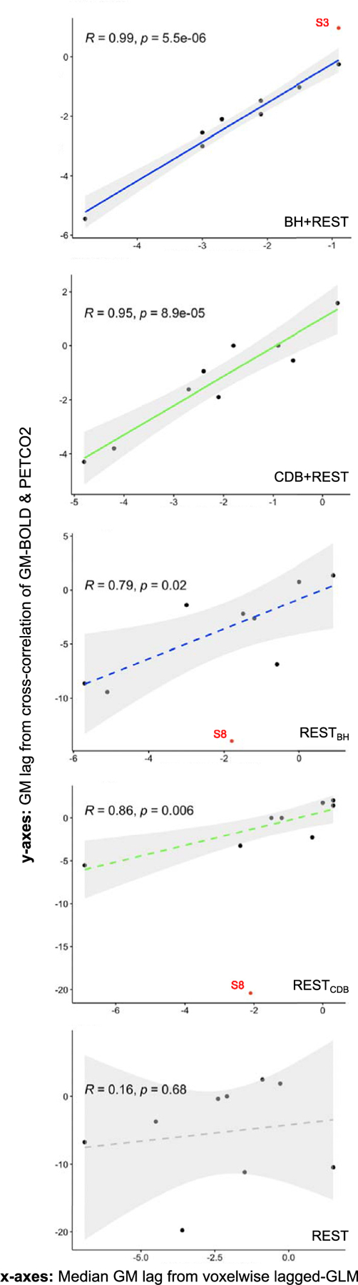
Correlation between two methods of identifying GM lag: the median lag over GM voxels from the voxelwise lagged-GLM analysis (x-axes) and a lag obtained from cross-correlation between the average GM-BOLD time-series and the P_ET CO₂hrf time-series (y-axes). Each dot represents one subject, and correlations are shown for each data segment. The gray shaded regions around the fit line indicate the 95% confidence interval of the correlation coefficient. Data points were classed as outliers (indicated by red dots) when a Cook’s distance was over 4/n, with n being the number of subjects. Outliers are not included in the correlation, but shown for reference. Note the different axes limits across plots. P-values are FDR corrected. Considering the shape of the lag distributions in Fig. 4, it is important to acknowledge that the use of the median as a summary metric may not be completely valid for all subjects and data segments. BH = breath holding, CDB = cued deep breathing, PETCO2 = Partial pressure of End Tidal CO2, GM = Gray Matter, BOLD = Blood Oxygenation Level Dependent.

References

- Bacigaluppi S, Dehdashti AR, Agid R, Krings T, Tymianski M, Mikulis DJ, 2009. The contribution of imaging in diagnosis, preoperative assessment, and follow-up of moyamoya disease. Neurosurg. Focus 26 (4), E3 March. [DOI] [PubMed] [Google Scholar]
- Benjamini Y, Hochberg Y, 1995. Controlling the False Discovery Rate: A Practical and Powerful Approach to Multiple Testing. J. R. Stat. Soc. Ser. B 57 (1), 289–300 January. [Google Scholar]
- Birn RM, Diamond JB, Smith MA, Bandettini PA, 2006. Separating respiratory-variation-related fluctuations from neuronal-activity-related fluctuations in fMRI. Neuroimage 31 (4), 1536–1548 July. [DOI] [PubMed] [Google Scholar]
- Birn RM, Smith MA, Jones TB, Bandettini PA, 2008. The respiration response function: The temporal dynamics of fMRI signal fluctuations related to changes in respiration. Neuroimage 40 (2), 644–654 April. [DOI] [PMC free article] [PubMed] [Google Scholar]
- Biswal BB, Kannurpatti SS, Rypma B, 2007. Hemodynamic scaling of fMRI-BOLD signal: validation of low-frequency spectral amplitude as a scalability factor. Magn. Reson. Imaging 25 (10), 1358–1369 December. [DOI] [PMC free article] [PubMed] [Google Scholar]
- Blockley NP, Driver ID, Francis ST, Fisher JA, Gowland PA, 2011. An improved method for acquiring cerebrovascular reactivity maps. Magn. Reson. Med 65 (5), 1278–1286 May. [DOI] [PubMed] [Google Scholar]
- Brian JE, 1998. Carbon dioxide and the cerebral circulation. Anesthesiology 88 (5), 1365–1386 American Society of Anesthesiologists01-May-. [DOI] [PubMed] [Google Scholar]
- Bright MG, Murphy K, 2017. Cleaning up the fMRI time series: Mitigating noise with advanced acquisition and correction strategies. NeuroImage 154, 1–3 Academic Press Inc.01-Jul-. [DOI] [PubMed] [Google Scholar]
- Bright MG, Murphy K, 2013. Reliable quantification of BOLD fMRI cerebrovascular reactivity despite poor breath-hold performance. Neuroimage 83, 559–568 December. [DOI] [PMC free article] [PubMed] [Google Scholar]
- Bright MG, Bulte DP, Jezzard P, Duyn JH, 2009. Characterization of regional heterogeneity in cerebrovascular reactivity dynamics using novel hypocapnia task and BOLD fMRI. Neuroimage 48 (1), 166–175 October. [DOI] [PMC free article] [PubMed] [Google Scholar]
- Bright MG, Donahue MJ, Duyn JH, Jezzard P, Bulte DP, 2011. The effect of basal vasodilation on hypercapnic and hypocapnic reactivity measured using magnetic resonance imaging. J. Cereb. Blood Flow Metab 31 (2), 426–438. [DOI] [PMC free article] [PubMed] [Google Scholar]
- Bright MG, Tench CR, Murphy K, 2017. Potential pitfalls when denoising resting state fMRI data using nuisance regression. Neuroimage 154, 159–168 July. [DOI] [PMC free article] [PubMed] [Google Scholar]
- Bright MG, Whittaker JR, Driver ID, Murphy K, 2020. Vascular physiology drives functional brain networks. Neuroimage 217 August. [DOI] [PMC free article] [PubMed] [Google Scholar]
- Bright MG, Bianciardi M, de Zwart JA, Murphy K, Duyn JH, 2014. Early anti-correlated BOLD signal changes of physiologic origin. Neuroimage 87, 287–296 February. [DOI] [PMC free article] [PubMed] [Google Scholar]
- Buterbaugh J, Wynstra C, Provencio N, Combs D, Gilbert M, Parthasarathy S, 2015. Cerebrovascular reactivity in young subjects with sleep apnea. Sleep 38 (2), 241–250 February. [DOI] [PMC free article] [PubMed] [Google Scholar]
- Caballero-Gaudes C, Reynolds RC, 2017. Methods for cleaning the BOLD fMRI signal HHS Public Access. Neuroimage 154, 128–149. [DOI] [PMC free article] [PubMed] [Google Scholar]
- Chang C, Glover GH, 2009. Relationship between respiration, end-tidal CO2, and BOLD signals in resting-state fMRI. Neuroimage 47 (4), 1381–1393 October. [DOI] [PMC free article] [PubMed] [Google Scholar]
- Chang C, Thomason ME, Glover GH, 2008. Mapping and correction of vascular hemodynamic latency in the BOLD signal. Neuroimage 43 (1), 90–102 October. [DOI] [PMC free article] [PubMed] [Google Scholar]
- Chen JE, et al. , 2020. Resting-state ‘physiological networks. Neuroimage 213, 116707 June. [DOI] [PMC free article] [PubMed] [Google Scholar]
- Christen T, Jahanian H, Ni WW, Qiu D, Moseley ME, Zaharchuk G, 2015. Noncontrast mapping of arterial delay and functional connectivity using resting-state functional MRI: A study in moyamoya patients. J. Magn. Reson. Imaging 41 (2), 424–430 February. [DOI] [PMC free article] [PubMed] [Google Scholar]
- Chu PPW, Golestani AM, Kwinta JB, Khatamian YB, Chen JJ, 2018. Characterizing the modulation of resting-state fMRI metrics by baseline physiology. Neuroimage 173, 72–87 June. [DOI] [PubMed] [Google Scholar]
- Churchill NW, Hutchison MG, Graham SJ, Schweizer TA, 2020. Cerebrovascular Reactivity After Sport Concussion: From Acute Injury to 1 Year After Medical Clearance. Front. Neurol 11, 558 July. [DOI] [PMC free article] [PubMed] [Google Scholar]
- Cohen AD, Wang Y, 2019. Improving the Assessment of Breath-Holding Induced Cerebral Vascular Reactivity Using a Multiband Multi-echo ASL/BOLD Sequence. Sci. Rep 9 (1), 5079 December. [DOI] [PMC free article] [PubMed] [Google Scholar]
- Conijn MMA, Hoogduin JM, van der Graaf Y, Hendrikse J, Luijten PR, Geerlings MI, 2012. Microbleeds, lacunar infarcts, white matter lesions and cerebrovascular reactivity - A 7T study. Neuroimage 59 (2), 950–956 January. [DOI] [PubMed] [Google Scholar]
- Conklin J, Fierstra J, Crawley AP, Han JS, Poublanc J, Mandell DM, Silver FL, Tymianski M, Fisher JA, Mikulis DJ, 2010. Impaired cerebrovascular reactivity with steal phenomenon is associated with increased diffusion in white matter of patients with Moyamoya disease. Stroke 41 (8), 1610–1616 August. [DOI] [PubMed] [Google Scholar]
- Cox RW, 1996. AFNI: Software for analysis and visualization of functional magnetic resonance neuroimages. Comput. Biomed. Res 29 (3), 162–173 June. [DOI] [PubMed] [Google Scholar]
- De Vis JB, Bhogal AA, Hendrikse J, Petersen ET, Siero JCW, 2018. Effect sizes of BOLD CVR, resting-state signal fluctuations and time delay measures for the assessment of hemodynamic impairment in carotid occlusion patients. Neuroimage 179, 530–539 October. [DOI] [PMC free article] [PubMed] [Google Scholar]
- Dlamini N, et al. , 2018. Breath-hold blood oxygen level-dependent MRI: A tool for the assessment of cerebrovascular reserve in children with moyamoya disease. Am. J. Neuroradiol 39 (9), 1717–1723. [DOI] [PMC free article] [PubMed] [Google Scholar]
- Donahue MJ, Strother MK, Lindsey KP, Hocke LM, Tong Y, Frederick BDB, 2016. Time delay processing of hypercapnic fMRI allows quantitative parameterization of cerebrovascular reactivity and blood flow delays. J. Cereb. Blood Flow Metab 36 (10), 1767–1779. [DOI] [PMC free article] [PubMed] [Google Scholar]
- Frossard J, Renaud O, “permuco: Permutation Tests for Regression, (Repeated Measures) ANOVA/ANCOVA and Comparison of Signals. R package version 1.1.0” 2019. [Google Scholar]
- Gaviria J, Rey G, Bolton T, Delgado J, Ville D, Vuilleumier P, 2020. Brain functional connectivity dynamics at rest in the aftermath of affective and cognitive challenges. Hum. Brain Mapp 42 (4) p. hbm.25277, November. [DOI] [PMC free article] [PubMed] [Google Scholar]
- Geranmayeh F, Wise RJS, Leech R, Murphy K, 2015. Measuring vascular reactivity with breath-holds after stroke: a method to aid interpretation of group-level BOLD signal changes in longitudinal fMRI studies. Hum. Brain Mapp 36 (5), 1755–1771 May. [DOI] [PMC free article] [PubMed] [Google Scholar]
- Glover GH, 2011. Overview of functional magnetic resonance imaging. Neurosurg. Clin. N. Am 22 (2), 133–139 vii, April. [DOI] [PMC free article] [PubMed] [Google Scholar]
- Golestani AM, Chen JJ, 2020. Controlling for the effect of arterial-CO2 fluctuations in resting-state fMRI: Comparing end-tidal CO2 clamping and retroactive CO2 correction. Neuroimage 216, 116874 August. [DOI] [PubMed] [Google Scholar]
- Golestani AM, Chang C, Kwinta JB, Khatamian YB, Chen JJean, 2015. Mapping the end-tidal CO2 response function in the resting-state BOLD fMRI signal: Spatial specificity, test-retest reliability and effect of fMRI sampling rate. Neuroimage 104, 266–277 January. [DOI] [PubMed] [Google Scholar]
- Golestani AM, Wei LL, Chen JJ, 2016. Quantitative mapping of cerebrovascular reactivity using resting-state BOLD fMRI: Validation in healthy adults. Neuroimage 138, 147–163 September. [DOI] [PMC free article] [PubMed] [Google Scholar]
- Greve DN, Brown GG, Mueller BA, Glover G, Liu TT, 2013. A Survey of the Sources of Noise in fMRI. Psychometrika 78 (3), 396–416 July. [DOI] [PubMed] [Google Scholar]
- Handwerker DA, Gazzaley A, Inglis BA, D’Esposito M, 2007. Reducing vascular variability of fMRI data across aging populations using a breathholding task. Hum. Brain Mapp 28 (9), 846–859. [DOI] [PMC free article] [PubMed] [Google Scholar]
- Harper AM, Glass HI, 1965. Effect of alterations in the arterial carbon dioxide tension on the blood flow through the cerebral cortex at normal and low arterial blood pressures. J Neurol Neurosurg Psychiatry 28 (5), 449–452 October. [DOI] [PMC free article] [PubMed] [Google Scholar]
- Hsu Y-Y, et al. , 2004. Blood oxygenation level-dependent MRI of cerebral gliomas during breath holding. J. Magn. Reson. Imaging 19 (2), 160–167 February. [DOI] [PubMed] [Google Scholar]
- Iranmahboob A, et al. , 2016. Vascular Reactivity Maps in Patients with Gliomas Using Breath-Holding BOLD fMRI. J. Neuroimaging 26 (2), 232–239 March. [DOI] [PMC free article] [PubMed] [Google Scholar]
- Jahanian H, et al. , 2017. Measuring vascular reactivity with resting-state blood oxygenation level-dependent (BOLD) signal fluctuations: A potential alternative to the breath-holding challenge? J. Cereb. Blood Flow Metab 37 (7), 2526–2538 July. [DOI] [PMC free article] [PubMed] [Google Scholar]
- Jenkinson M, Smith S, 2001. A global optimisation method for robust affine registration of brain images. Med. Image Anal 5 (2), 143–156 June. [DOI] [PubMed] [Google Scholar]
- Jenkinson M, Bannister P, Brady M, Smith S, 2002. Improved Optimization for the Robust and Accurate Linear Registration and Motion Correction of Brain Images. Neuroimage 17 (2), 825–841 October. [DOI] [PubMed] [Google Scholar]
- Jenkinson M, Beckmann CF, Behrens TEJ, Woolrich MW, Smith SM, 2012. FSL. Neuroimage 62 (2), 782–790 August. [DOI] [PubMed] [Google Scholar]
- Juttukonda MR, Donahue MJ, 2019. Neuroimaging of vascular reserve in patients with cerebrovascular diseases. Neuroimage 187, 192–208 February. [DOI] [PMC free article] [PubMed] [Google Scholar]
- Kannurpatti SS, Biswal BB, 2008. Detection and scaling of task-induced fMRI-BOLD response using resting state fluctuations. Neuroimage 40 (4), 1567–1574 May. [DOI] [PMC free article] [PubMed] [Google Scholar]
- Kasprowicz M, et al. , 2012. Time Constant of the Cerebral Arterial Bed in Normal Subjects. Ultrasound Med. Biol 38 (7), 1129–1137 July. [DOI] [PubMed] [Google Scholar]
- Kassambara A, “ggpubr: ‘ggplot2’ Based Publication Ready Plots. R package version 0.4.0,” 2020. [Google Scholar]
- Kassinopoulos M, Mitsis GD, 2019. Identification of physiological response functions to correct for fluctuations in resting-state fMRI related to heart rate and respiration. Neuroimage 202, 116150 November. [DOI] [PubMed] [Google Scholar]
- Kastrup A, Krüger G, Neumann-Haefelin T, Moseley ME, 2001. Assessment of cerebrovascular reactivity with functional magnetic resonance imaging: Comparison of CO2 and breath holding. Magn. Reson. Imaging 19 (1), 13–20 January. [DOI] [PubMed] [Google Scholar]
- Kay KN, David SV, Prenger RJ, Hansen KA, Gallant JL, 2008. Modeling low-frequency fluctuation and hemodynamic response timecourse in event-related fMRI. Hum. Brain Mapp 29 (2), 142–156 February. [DOI] [PMC free article] [PubMed] [Google Scholar]
- Kim SG, Ogawa S, 2012. Biophysical and physiological origins of blood oxygenation level-dependent fMRI signals. Journal of Cerebral Blood Flow and Metabolism 32 (7), 1188–1206 SAGE PublicationsJul-. [DOI] [PMC free article] [PubMed] [Google Scholar]
- Krainik A, Hund-Georgiadis M, Zysset S, Von Cramon DY, 2005. Regional impairment of cerebrovascular reactivity and BOLD signal in adults after stroke. Stroke 36 (6), 1146–1152 June. [DOI] [PubMed] [Google Scholar]
- Li X, Morgan PS, Ashburner J, Smith J, Rorden C, 2016. The first step for neuroimaging data analysis: DICOM to NIfTI conversion. J. Neurosci. Methods 264, 47–56 May. [DOI] [PubMed] [Google Scholar]
- Lipp I, Murphy K, Caseras X, Wise RG, 2015. Agreement and repeatability of vascular reactivity estimates based on a breath-hold task and a resting state scan. Neuroimage 113, 387–396 June. [DOI] [PMC free article] [PubMed] [Google Scholar]
- Liu P, De Vis JB, 2019. Cerebrovascular reactivity (CVR) MRI with CO2 challenge: A technical review. Neuroimage 187, 104–115 February. [DOI] [PMC free article] [PubMed] [Google Scholar]
- Liu P, Li Y, Pinho M, Park DC, Welch BG, Lu H, 2017. Cerebrovascular reactivity mapping without gas challenges. Neuroimage 146, 320–326 February. [DOI] [PMC free article] [PubMed] [Google Scholar]
- Liu P, et al. , 2020. Cerebrovascular reactivity mapping using intermittent breath modulation. Neuroimage 215, 116787 July. [DOI] [PMC free article] [PubMed] [Google Scholar]
- Liu TT, 2013. Neurovascular factors in resting-state functional MRI. Neuroimage 80, 339–348 October. [DOI] [PMC free article] [PubMed] [Google Scholar]
- Liu TT, 2016. Noise contributions to the fMRI signal: An overview. Neuroimage 143, 141–151 December. [DOI] [PubMed] [Google Scholar]
- Lynch CJ, et al. , 2020. Prevalent and sex-biased breathing patterns modify functional connectivity MRI in young adults. Nat. Commun 11 (1). [DOI] [PMC free article] [PubMed] [Google Scholar]
- Madjar C, Gauthier CJ, Bellec P, Birn RM, Brooks JCW, Hoge RD, 2012. Task-related BOLD responses and resting-state functional connectivity during physiological clamping of end-tidal CO 2. Neuroimage 61 (1), 41–49 May. [DOI] [PubMed] [Google Scholar]
- Magon S, Basso G, Farace P, Ricciardi GK, Beltramello A, Sbarbati A, 2009. Reproducibility of BOLD signal change induced by breath holding. Neuroimage 45 (3), 702–712 April. [DOI] [PubMed] [Google Scholar]
- McSwain SD, et al. , 2010. End-tidal and arterial carbon dioxide measurements correlate across all levels of physiologic dead space. Respir. Care 55 (3), 288–293 March. [PMC free article] [PubMed] [Google Scholar]
- Meng L, Gelb AW, 2015. Regulation of cerebral autoregulation by carbon dioxide. Anesthesiology 122 (1), 196–205 Lippincott Williams and Wilkins01-Jan-. [DOI] [PubMed] [Google Scholar]
- Moia S, Stickland RC, Ayyagari A, Termenon M, Caballero-Gaudes C, Bright MG, 2020. Voxelwise optimization of hemodynamic lags to improve regional CVR estimates in breath-hold fMRI∗ In: 2020 42nd Annual International Conference of the IEEE Engineering in Medicine & Biology Society (EMBC), pp. 1489–1492. [DOI] [PubMed] [Google Scholar]
- Moia S, et al. , 2021. ICA-based denoising strategies in breath-hold induced cerebrovascular reactivity mapping with multi echo BOLD fMRI. Neuroimage 233, 117914 June. [DOI] [PMC free article] [PubMed] [Google Scholar]
- Murphy K, Harris AD, Wise RG, 2011. Robustly measuring vascular reactivity differences with breath-hold: Normalising stimulus-evoked and resting state BOLD fMRI data. Neuroimage 54 (1), 369–379. [DOI] [PubMed] [Google Scholar]
- Murphy K, Birn RM, Bandettini PA, 2013. Resting-state fMRI confounds and cleanup. Neuroimage 80, 349–359 October. [DOI] [PMC free article] [PubMed] [Google Scholar]
- Ni L, et al. , 2017. The value of resting-state functional MRI in subacute ischemic stroke: Comparison with dynamic susceptibility contrast-enhanced perfusion MRI. Sci. Rep 7 (1), 1–8 January. [DOI] [PMC free article] [PubMed] [Google Scholar]
- Ni L, et al. , 2020. Lower Cerebrovascular Reactivity Contributed to White Matter Hyperintensity-Related Cognitive Impairment: A Resting-StateFunctionalMRIStudy. J. Magn. Reson. Imaging p. jmri.27376, September. [DOI] [PubMed] [Google Scholar]
- Nikolaou F, Orphanidou C, Wise RG, Mitsis GD, 2015. Arterial CO2 effects modulate dynamic functional connectivity in resting-state fMRI In: Proceedings of the Annual International Conference of the IEEE Engineering in Medicine and Biology Society, EMBS, pp. 1809–1812 2015-November. [DOI] [PubMed] [Google Scholar]
- Pillai JJ, Mikulis DJ, 2014. Cerebrovascular Reactivity Mapping: An Evolving Standard for Clinical Functional Imaging. AJNR. Am. J. Neuroradiol 1–7. [DOI] [PMC free article] [PubMed] [Google Scholar]
- Pillai JJ, 2011. Clinical utility of cerebrovascular reactivity mapping in patients with low grade gliomas. World J. Clin. Oncol 2 (12), 397. [DOI] [PMC free article] [PubMed] [Google Scholar]
- Pinto J, Jorge J, Sousa I, Vilela P, Figueiredo P, 2016. Fourier modeling of the BOLD response to a breath-hold task: Optimization and reproducibility. Neuroimage 135, 223–231 July. [DOI] [PubMed] [Google Scholar]
- Pinto J, Bright MG, Bulte DP, Figueiredo P, 2021. Cerebrovascular Reactivity Mapping Without Gas Challenges: A Methodological Guide. Front. Physiol 11, 1711 January. [DOI] [PMC free article] [PubMed] [Google Scholar]
- Poublanc J, et al. , 2013. Vascular Steal Explains Early Paradoxical Blood Oxygen Level-Dependent Cerebrovascular Response in Brain Regions with Delayed Arterial Transit Times. Cerebrovasc. Dis. Extra 3 (1), 55–64 April. [DOI] [PMC free article] [PubMed] [Google Scholar]
- Poulin MJ, Liang PJ, Robbins PA, 1996. Dynamics of the cerebral blood flow response to step changes in end-tidal PCO2 and PO2 in humans. J. Appl. Physiol 81 (3), 1084–1095. [DOI] [PubMed] [Google Scholar]
- Poulin MJ, Liang PJ, Robbins PA, 1998. Fast and slow components of cerebral blood flow response to step decreases in end-tidal PCO2 in humans. J. Appl. Physiol 85 (2), 388–397. [DOI] [PubMed] [Google Scholar]
- Power JD, Barnes KA, Snyder AZ, Schlaggar BL, Petersen SE, 2012. Spurious but systematic correlations in functional connectivity MRI networks arise from subject motion. Neuroimage 59 (3), 2142–2154 February. [DOI] [PMC free article] [PubMed] [Google Scholar]
- Power JD, Mitra A, Laumann TO, Snyder AZ, Schlaggar BL, Petersen SE, 2014. Methods to detect, characterize, and remove motion artifact in resting state fMRI. Neuroimage 84, 320–341 January. [DOI] [PMC free article] [PubMed] [Google Scholar]
- Power JD, Plitt M, Laumann TO, Martin A, 2017. Sources and implications of whole-brain fMRI signals in humans. Neuroimage 146, 609–625 February. [DOI] [PMC free article] [PubMed] [Google Scholar]
- Power JD, et al. , 2018. Ridding fMRI data of motion-related influences: Removal of signals with distinct spatial and physical bases in multiecho data. Proc. Natl. Acad. Sci. USA 115 (9), E2105–E2114. [DOI] [PMC free article] [PubMed] [Google Scholar]
- Prilipko O, Huynh N, Thomason ME, Kushida CA, Guilleminault C, 2014. An fMRI study of cerebrovascular reactivity and perfusion in obstructive sleep apnea patients before and after CPAP treatment. Sleep Med 15 (8), 892–898. [DOI] [PubMed] [Google Scholar]
- R Core Team, 2019. R: A language and Environment For Statistical Computing R Foundation for Statistical Computing, Vienna, Austria: 2019. [Google Scholar]
- Raut RV, Nair VA, Sattin JA, Prabhakaran V, 2016. Hypercapnic evaluation of vascular reactivity in healthy aging and acute stroke via functional MRI. NeuroImage Clin 12, 173–179. [DOI] [PMC free article] [PubMed] [Google Scholar]
- Schubert GA, et al. , 2009. Cerebrovascular insufficiency as the criterion for revascularization procedures in selected patients: A correlation study of xenon contrast-enhanced CT and PWI. Neurosurg. Rev 32 (1), 29–36. [DOI] [PubMed] [Google Scholar]
- Secchinato KF, Da Silva PHR, Camargo APA, Pontes-Neto OM, Leoni RF, 2019. Cerebrovascular reactivity mapping without hypercapnic challenge in patients with carotid artery stenosis. Rev. Bras. Física Médica 13 (2), 62 December. [Google Scholar]
- Sidak Z, 1967. Rectangular Confidence Regions for the Means of Multivariate Normal Distributions. J. Am. Stat. Assoc 62 (318), 626 June. [Google Scholar]
- Siegel JS, Snyder AZ, Ramsey L, Shulman GL, Corbetta M, 2016. The effects of hemodynamic lag on functional connectivity and behavior after stroke. J. Cereb. Blood Flow Metab 36 (12), 2162–2176 December. [DOI] [PMC free article] [PubMed] [Google Scholar]
- Smith SM, et al. , 2004. Advances in functional and structural MR image analysis and implementation as FSL. NeuroImage 23, S208–S219. [DOI] [PubMed] [Google Scholar]
- Smith SM, 2002. Fast robust automated brain extraction. Hum. Brain Mapp 17 (3), 143–155 November. [DOI] [PMC free article] [PubMed] [Google Scholar]
- Sousa I, Vilela P, Figueiredo P, 2014. Reproducibility of hypocapnic cerebrovascular reactivity measurements using BOLD fMRI in combination with a paced deep breathing task. Neuroimage 98, 31–41 September. [DOI] [PubMed] [Google Scholar]
- Takano Y, Sakamoto O, Kiyofuji C, Ito K, 2003. A comparison of the end-tidal CO2 measured by portable capnometer and the arterial PCO2 in spontaneously breathing patients. Respir Med 97 (5), 476–481 May. [DOI] [PubMed] [Google Scholar]
- Taneja K, et al. , 2019. Evaluation of cerebrovascular reserve in patients with cerebrovascular diseases using resting-state MRI: A feasibility study. Magn. Reson. Imaging 59, 46–52 June. [DOI] [PMC free article] [PubMed] [Google Scholar]
- Tchistiakova E, Anderson ND, Greenwood CE, Macintosh BJ, 2014. Combined effects of type 2 diabetes and hypertension associated with cortical thinning and impaired cerebrovascular reactivity relative to hypertension alone in older adults. NeuroImage Clin 5, 36–41. [DOI] [PMC free article] [PubMed] [Google Scholar]
- Thomas BP, Liu P, Aslan S, King KS, van Osch MJP, Lu H, 2013. Physiologic underpinnings of negative BOLD cerebrovascular reactivity in brain ventricles. Neuroimage 83, 505–512 December. [DOI] [PMC free article] [PubMed] [Google Scholar]
- Thomason ME, Burrows BE, Gabrieli JDE, Glover GH, 2005. Breath holding reveals differences in fMRI BOLD signal in children and adults. Neuroimage 25 (3), 824–837 April. [DOI] [PubMed] [Google Scholar]
- Thomason ME, Foland LC, Glover GH, 2007. Calibration of BOLD fMRI using breath holding reduces group variance during a cognitive task. Hum. Brain Mapp 28 (1), 59–68 January. [DOI] [PMC free article] [PubMed] [Google Scholar]
- Tisdall MD, Reuter M, Qureshi A, Buckner RL, Fischl B, van der Kouwe AJW, 2016. Prospective motion correction with volumetric navigators (vNavs) reduces the bias and variance in brain morphometry induced by subject motion. Neuroimage 127, 11–22 February. [DOI] [PMC free article] [PubMed] [Google Scholar]
- Tong Y, Bergethon PR, de B, Frederick B, 2011. An improved method for mapping cerebrovascular reserve using concurrent fMRI and near-infrared spectroscopy with Regressor Interpolation at Progressive Time Delays (RIPTiDe). Neuroimage 56 (4), 2047–2057 June. [DOI] [PMC free article] [PubMed] [Google Scholar]
- Tong Y, de B, Frederick B, 2014. Tracking cerebral blood flow in BOLD fMRI using recursively generated regressors. Hum. Brain Mapp 35 (11), 5471–5485 November. [DOI] [PMC free article] [PubMed] [Google Scholar]
- Tong Y, Hocke LM, Frederick BB, 2019. Low Frequency Systemic Hemodynamic ‘Noise’ in Resting State BOLD fMRI: Characteristics, Causes, Implications, Mitigation Strategies, and Applications. Front. Neurosci 13, 787 no. JULAug. [DOI] [PMC free article] [PubMed] [Google Scholar]
- Tsvetanov KA, Henson RNA, Tyler LK, Davis SW, Shafto MA, Taylor JR, Williams N, Cam-Can, Rowe JB, 2015. The effect of ageing on fMRI: Correction for the confounding effects of vascular reactivity evaluated by joint fMRI and MEG in 335 adults. Hum Brain Mapp 36 (6), 2248–2269 February. [DOI] [PMC free article] [PubMed] [Google Scholar]
- Tung KC, Uh J, Mao D, Xu F, Xiao G, Lu H, 2013. Alterations in resting functional connectivity due to recent motor task. Neuroimage 78, 316–324 September. [DOI] [PMC free article] [PubMed] [Google Scholar]
- Urback AL, MacIntosh BJ, Goldstein BI, 2017. Cerebrovascular reactivity measured by functional magnetic resonance imaging during breath-hold challenge: A systematic review. Neurosci. Biobeh. Rev 79, 27–47 Elsevier Ltd01-Aug-. [DOI] [PubMed] [Google Scholar]
- Van Oers CAMM, Van Der Worp HB, Kappelle LJ, Raemaekers MAH, Otte WM, Dijkhuizen RM, 2018. Etiology of language network changes during recovery of aphasia after stroke. Sci. Rep 8 (1) December. [DOI] [PMC free article] [PubMed] [Google Scholar]
- Whittaker JR, Driver ID, Venzi M, Bright MG, Murphy K, 2019. Cerebral Autoregulation Evidenced by Synchronized Low Frequency Oscillations in Blood Pressure and Resting-State fMRI. Front. Neurosci 13, 433 May. [DOI] [PMC free article] [PubMed] [Google Scholar]
- Wickham H, 2016. ggplot2: Elegant Graphics For Data Analysis Springer-Verlag, New York. [Google Scholar]
- Wise RG, Ide K, Poulin MJ, Tracey I, 2004. Resting fluctuations in arterial carbon dioxide induce significant low frequency variations in BOLD signal. Neuroimage 21 (4), 1652–1664 April. [DOI] [PubMed] [Google Scholar]
- Woolrich MW, et al. , 2009. Bayesian analysis of neuroimaging data in FSL. Neuroimage 45 (1 Suppl), S173–S186 March. [DOI] [PubMed] [Google Scholar]
- Wu PH, et al. , 2020. MRI evaluation of cerebrovascular reactivity in obstructive sleep apnea. J. Cereb. Blood Flow Metab 40 (6), 1328–1337 June. [DOI] [PMC free article] [PubMed] [Google Scholar]
- Zacà D, Jovicich J, Nadar SR, Voyvodic JT, Pillai JJ, 2014. Cerebrovascular reactivity mapping in patients with low grade gliomas undergoing presurgical sensorimotor mapping with BOLD fMRI. J. Magn. Reson. Imaging 40 (2), 383–390 August. [DOI] [PMC free article] [PubMed] [Google Scholar]
- Zhang Y, Brady M, Smith S, 2001. Segmentation of brain MR images through a hidden Markov random field model and the expectation-maximization algorithm. IEEE Trans. Med. Imaging 20 (1), 45–57. [DOI] [PubMed] [Google Scholar]
- Zhao P, et al. , 2009. Vasoreactivity and peri-infarct hyperintensities in stroke. Neurology 72 (7), 643–649 February. [DOI] [PMC free article] [PubMed] [Google Scholar]
Associated Data
This section collects any data citations, data availability statements, or supplementary materials included in this article.