

Abstract
The coordination of interconnected elements across the different layers of the supply chain is essential for all industrial processes and the key to optimal decision-making. Yet, the modeling and optimization of such interdependent systems are still burdensome. In this paper, we address the simultaneous modeling and optimization of medium-term planning and short-term scheduling problems under demand uncertainty using mixed-integer bi-level multi-follower programming and data-driven optimization. Bi-level multi-follower programs model the natural hierarchy between different layers of supply chain management holistically, while scenario analysis and data-driven optimization allow us to retrieve the guaranteed feasible solutions of the integrated formulation under various demand considerations. We address the data-driven optimization of this challenging class of problems using the DOMINO framework, which was initially developed to solve single-leader single-follower bi-level optimization problems to guaranteed feasibility. This framework is extended to solve single-leader multi-follower stochastic formulations and its performance is characterized by well-known single and multi-product process scheduling case studies. Through our data-driven algorithmic approach, we present guaranteed feasible solutions to linear and nonlinear mixed-integer bi-level formulations of simultaneous planning and scheduling problems and further characterize the effects of the scheduling level complexity on the solution performance, which spans over several hundred continuous and binary variables, and thousands of constraints.
Keywords: Data-driven Optimization, Bi-level Programming, Stochastic Analysis, Integrated Planning and Scheduling, Demand Uncertainty, Feasibility
1. Introduction
Current industrial processes require the coordination of many interconnected pieces that involve multi-dimensional, multi-purpose, and multi-product systems. Across the different layers of supply chain management, starting from the supply chain structure to production planning and scheduling, the optimal coordination of each element and their robust response to changing market conditions is essential for increasing efficiency, resiliency, productivity, and profitability of any enterprise (Papageorgiou, 2009; Maravelias & Sung, 2009; Grossmann, 2012; Avraamidou & Pistikopoulos, 2017). Yet, decision-making in such multi-level networks that integrate long-term decisions (i.e., supply chain problem) with medium-term tactical (i.e., planning problem) and short-term production decisions (i.e., scheduling problem) is a challenging task.
The difficulties in such enterprise-wide decision-making problems are extensively discussed by Grossmann (2005) and later again in 2012 (Grossmann, 2012) in which the key issues are summarized as follows: (1) The modeling challenge (i.e., the type of planning and scheduling models, linear vs nonlinear); (2) the multi-scale optimization challenge (i.e., the coordination between decisions that are taken over different timescales, months vs days, days vs hours); (3) the uncertainty challenge (i.e., handling stochasticity from various sources); and, (4) the algorithmic challenge (i.e., developing effective and efficient algorithms that can solve complex optimization problems).
Due to the multi-faceted nature of these challenges, a typical approach for solving integrated planning and scheduling problems is to address them sequentially, starting from higher-level decisions first and tackling lower-level decisions later. For example, a sequential solution strategy for an integrated planning and scheduling problem will be as follows:
Market conditions are analyzed, and the production targets are set for the desired goods to meet the product demand. (Planning Level)
Production schedules outlining the optimal sequencing of tasks and material use are retrieved for meeting the production targets. (Scheduling Level)
Although this strategy overcomes a portion of the stated challenges, the sequential approach is an optimistic estimate for the planning level decisions because it disregards the interconnectivity between the scheduling layer (Grossmann, 2005). Particularly, the planning level decisions solely taken based on the market conditions (i.e., demand profiles) and without any input from the scheduling level will exceed the production capacity limits of the units at the scheduling layer. As a result, the optimal coordination of tasks for producing the desired goods will ultimately fail and become infeasible without being able to meet the production targets and the demand (Figure 1A). Hence, globally optimal solutions for such interdependent systems can only be achieved if the interconnections between different layers of supply chain planning are handled simultaneously rather than sequentially (Maravelias & Sung, 2009).
Figure 1:
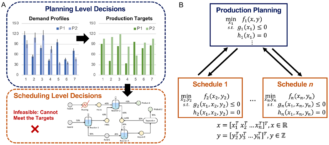
(A) Illustration of a major issue with sequential solution algorithms for integrated planning and scheduling problems. When planning level decisions are taken independently of the lower-level information, the scheduling feasibility can be violated. (B) Recasting integrated planning and scheduling problems using mixed-integer bi-level multi-follower programs to avoid lower-level infeasibility.
Bi-level programming offers a compact and holistic modeling approach for handling the natural hierarchy that exists between different layers of supply chain management (Avraamidou & Pistikopoulos, 2019b). Specifically, planning and scheduling optimization problems with seasonal demand variability can be expressed holistically within a hierarchical structure, where optimal decisions at the planning level (first-level optimization problem) provide constraints for the detailed decision making at the scheduling levels (second-level optimization problems), typically posed as bi-level multi-follower optimization problems (Figure 1B) (Chu et al., 2015; Dogan & Grossmann, 2006; Li & Ierapetritou, 2009). These problems can involve decisions in both discrete and continuous variables, therefore are referred to as mixed-integer bi-level multi-follower programming problems (BMF-MIP).
Figure 1B illustrates the natural hierarchy and dependence between the planning and scheduling optimization problems; where x1 is a vector of the leader’s (planning problem) continuous variables, x2 to xn are vectors of the followers (scheduling problems) continuous variables, and y2 to yn are vectors of the followers’ integer variables. Note that the scheduling decision problems all belong to the same optimization level, and each depends on the upper-level decisions x1, while the planning problem’s objective function also depends on variables decided by the scheduling problems (x, y).
Solution approaches for bi-level optimization with both integer and continuous variables have been mainly developed for the case of single-leader single-follower problems (Avraamidou & Pistikopoulos, 2019c; Mitsos, 2010; Saharidis & Ierapetritou, 2009; Gümüş & Floudas, 2005; Kleniati & Adjiman, 2015; Avraamidou & Pistikopoulos, 2019a; Beykal et al., 2020a; Avraamidou et al., 2018), while the case of single-leader multiple-followers has not received a lot of attention from the research community. Attempts to solve multifollower problems focused on the linear continuous case (Shi et al., 2007; Lu et al., 2006, 2007; Calvete & Galé, 2007), while multi-parametric approaches have been developed for the linear continuous (Faísca et al., 2009) and mixed-integer cases (Avraamidou & Pistikopoulos, 2018). To our knowledge, a very limited number of heuristic approaches exist for the solution of nonlinear mixed-integer multi-follower problems which do not guarantee global optimality nor feasibility (Sinha et al., 2014).
This motivates us to explore new algorithmic approaches that can tackle the challenging optimization problem presented in Figure 1B. Especially, the recent advances in data analytics and the increasing use of these techniques in process systems engineering strikes as an attractive methodology for addressing BMF-MIP problems. Previously, data-driven modeling and optimization have shown to be effective in solving nonlinear (Mistry et al., 2020; Beykal et al., 2018b; Kim & Boukouvala, 2020; Cozad et al., 2014; Bi et al., 2020), multi-objective (Beykal et al., 2018a; Schweidtmann et al., 2018), bi-level single-follower (Beykal et al., 2020a; Avraamidou et al., 2018), and multi-parametric optimization problems (Katz et al., 2020), as well as for addressing the optimization of numerically infeasible differential algebraic equations (Beykal et al., 2020b). Few studies also demonstrated the use of data-driven approaches in integrated planning and scheduling applications where scheduling level feasible regions are approximated using surrogate functions (Sung & Maravelias, 2007, 2009) and classification algorithms (Dias & Ierapetritou, 2019). We have also recently demonstrated that data-driven algorithms can be used to solve deterministic integrated planning and scheduling problems (Beykal et al., 2021).
In this work, our goal is to benefit from the strengths of optimization theory and data-driven analysis to provide guaranteed feasible solutions to integrated planning and scheduling problems under demand uncertainty. The novelty of our work comes from following a hybrid approach to overcome the aforementioned challenges for integrated planning and scheduling problems. For this purpose, we model the integrated planning and scheduling problems as BMF-MIP under uncertainty and handle the demand stochasticity at the planning level through scenario analysis. We explore both linear and nonlinear bi-level formulations and present a multi-follower data-driven optimization strategy that utilizes the DOMINO algorithm (Beykal et al., 2020a) for finding the near-optimal solutions of bi-level mixed-integer problems with a feasibility guarantee. Our approach benefits from using surrogate-based and/or data-driven optimization strategies at the planning level while keeping the original mixed-integer scheduling formulation intact at the lower level.
The rest of the manuscript is organized as follows. In Section 2, we provide a detailed description of the problem formulation and its data-driven optimization using the DOMINO algorithm. Then in Section 3, the details of the computational case studies are provided with optimization results presented in Section 4. Final remarks on the manuscript are provided in Section 5.
2. Methodology
2.1. Stochastic Bi-level Multi-Follower Formulation
We formulate the stochastic integrated planning and scheduling problems in the following bi-level form
| (1) |
The leader (first level) is the planning problem represented with the minimization of the total stochastic cost of planning and inventory balance equations per scenario m, whereas the follower (second level) considers the scheduling problem with the minimization of the production cost per planning period t and scenario m. Our goal is to find the best set of production targets per planning period per product in a given problem while satisfying the product demand, inventory levels, and the optimality of the scheduling level. The detailed formulations of each optimization level are provided below.
2.1.1. The Leader Problem: Planning Model
The planning level equations are adapted from the deterministic formulation presented in Li & Ierapetritou (2009) without any backorder costs. The objective function of the planning level considers the summation of the total cost of planning per scenario m over the total number of scenarios Nm and their respective probability of occurrence φm.
| (2) |
The total cost of planning per scenario is defined as the summation of the inventory cost for the desired products (i.e., product states) and the production cost calculated from minimizing the scheduling problem at the lower level across the entire planning horizon with a definite number of periods t ∈ 1, …, T per scenario.
| (3) |
The inventory cost of products (InventoryCostt,m) is calculated by the summation of inventory levels of product states s ∈ SP per planning period per scenario and multiplying each level with their respective inventory prices (hs). Note that the subscript indices refer to the information coming from the lower-level scheduling formulation (i.e., states s), whereas superscript indices refer to the information coming from the upper-level problem definition (i.e., planning period t and scenario m).
| (4) |
The inventory levels of product states at the end of the current planning period is calculated by adding the ending inventory level from the previous period and the current production target , then subtracting the product demand level at the current planning period t.
| (5) |
All variables in Equation 5 are greater than or equal to zero across the entire planning horizon and demand scenarios with and If the inventory levels of any products fall to a negative value at any planning period in a given scenario m, the minimum inventory level of each product across the entire planning horizon is calculated, and all inventory levels per planning period are penalized by adding the missing minimum inventory level. This way the minimum inventory becomes zero and the rest of the inventory levels are kept positive while the direct cost of penalization is added to the objective through an increase in the inventory cost. This is also critical to ensure the product demands are satisfied. As Equation 5 needs to be greater than or equal to zero, this expression can be rearranged to define the constraint for demand satisfaction for all products in all stochastic scenarios at every planning period.
| (6) |
It is also important to note that the inventory and demand levels of each product given in Equation 5 can be different across different scenarios. However, the production targets of each product until the final planning period will be the same across different scenarios, and the goal is to find the best set of targets that will satisfy uncertain product demands that are represented with different scenarios using a data-driven approach. The final production target in the solution can be different across scenarios because we consider a cyclic formulation for the integrated planning and scheduling problem where the initial inventory level of the first planning period is assumed to be greater than zero. Thus, the production target at the final planning period (t = T) should ensure that the final day demand is satisfied and the initial inventory level of the next planning horizon is produced to achieve continuity. This can be mathematically expressed with the following expression using Equation 5:
| (7) |
As the planning problem is considered under a definite number of periods t ∈ 1, …, T, Equation 5 can further be used to replace with:
| (8) |
This replacement is followed in a cascaded approach until we reach the first planning period t = 1:
| (9) |
This procedure will eliminate all inventory variables and the remaining expression for the production targets at the final planning period will only be determined from the total demand across the entire planning horizon and the previous targets per scenario, as shown in Equation 10.
| (10) |
Since the production target of the desired products at the final planning period is deterministically calculated using Equation 10, it is possible to get negative values when the sum of previous production targets exceeds the total demand. This indicates that there is an excess amount of material to satisfy the demand with no need to produce any products in the final period. Hence, if the final production target for any product falls into a negative value, this target is set to be equal to zero.
2.1.2. The Follower Problem: Scheduling Model
We use the continuous-time formulation (Ierapetritou & Floudas, 1998; Li & Ierapetritou, 2009) for modeling the scheduling problem. The model is modified to solve for every planning period and scenario in the stochastic formulation. The lower-level is a multi-follower problem where for a given scenario, the scheduling formulation is sequentially solved over the entire planning horizon, starting from the initial planning day t = 1 ending with t = T.
The objective of the follower problem is to minimize the production cost of batch process scheduling which considers the fixed costs of tasks in the active units and the variable cost of tasks that undertake variable amounts of materials per planning period t per scenario m:
| (11) |
The scheduling formulation includes allocation constraints that limit the number of tasks that can be done in each unit j at a given event point n.
| (12) |
Units in the batch process system have bounds defining the maximum capacity of material that can be undertaken in unit j when performing task i and the minimum amount of material required to start task i in unit j.
| (13) |
Each state s can be stored up to a limited capacity at each event point n.
| (14) |
The material balance accounts for the production and consumption of each state s at a given event point n, as well as the amount of states from the previous event point.
| (15) |
In the case where n = 1, the amount of state s from the previous event point is equal to the initial state amounts. The material balance accounts for this initial amount and the consumption between event points n = 0 and n = 1.
| (16) |
Duration constraints account for the time duration of task i in unit j at an event point n and consider both the fixed and variable processing times.
| (17) |
The constant and variable terms of the processing time of task i in unit j are defined in Equations 18 and 19, respectively. It is assumed that there is a 33% variation around the mean processing time . This corresponds to a minimum processing time of and a maximum processing time of . Please note that the constant term is also equal to the minimum processing time, as shown in Equation 18.
| (18) |
| (19) |
The sequencing between the starting and final times for the tasks and units are defined by the sequence constraints. The sequencing constraints are defined based on having the same task in the same unit (Equations 20–22), different tasks in the same unit (Equation 23), different tasks in different units (Equation 24), and completion of previous tasks (Equation 25).
| (20) |
| (21) |
| (22) |
| (23) |
| (24) |
| (25) |
Time horizon constraints are included to ensure the start and the final processing times do not exceed the scheduling time horizon at a given day.
| (26) |
| (27) |
Finally, a constraint is added to ensure the feasibility of the scheduling problems when the leader problem decides on the production targets for the product states where the final amount of product states should be greater than or equal to the production target (Equation 28). This constraint integrates the planning and scheduling levels where the decision variables of the leader problem participate in the lower-level problem and dictates that unless the scheduling level can produce the desired products, the solution of the integrated problem will be infeasible. In the next section, we discuss how stochasticity in the product demands is handled via scenario analysis.
| (28) |
2.2. Scenario Analysis
The stochastic demands for the integrated planning and scheduling problem are represented with scenarios. As the increasing number of scenarios gives us a better understanding of how the system will respond to changing demand values, it is not practical to solve infinitely many scenarios. To that perspective, we assume a normally distributed demand profile with a mean distribution selected to be within the range of the amount of material that can be processed by any task required to start operating a unit in the scheduling problem with a 20% standard deviation around the selected mean demand. A total of 10,000 candidate scenarios are created randomly for the analysis. From these 10,000 scenarios, we further randomly sample 9 representative cases to construct the scenario tree shown in Figure 2.
Figure 2:
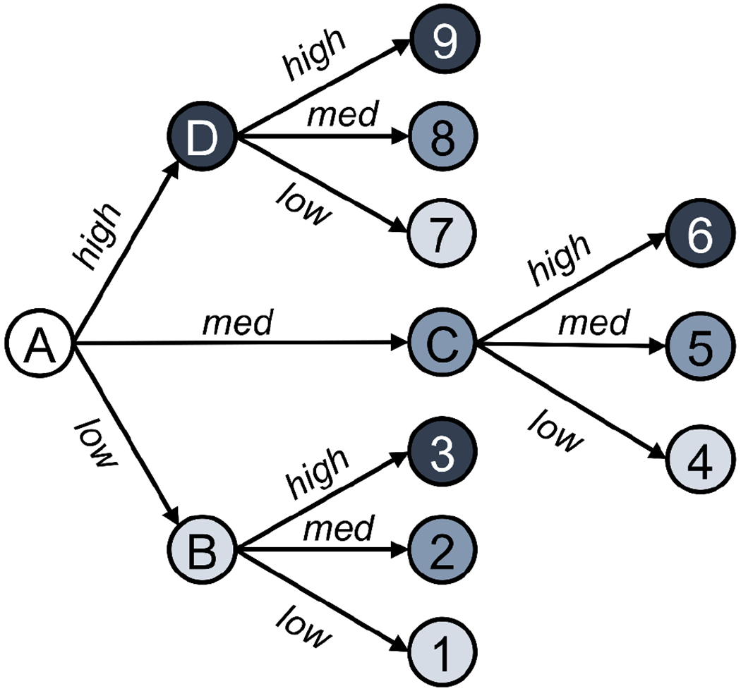
Scenario tree for stochastic analysis with 9 scenarios. Node A represents the known first-day demand and Nodes B, C, and D represent the product demand levels of Day 2 and 3. The terminal nodes of the scenario tree represent the product demand levels of Day 4-7 following the considered scenarios in Nodes B, C, and D.
For all the computational studies, we assume a fixed planning period of 7 days with the first-day demand for all products to be known deterministically. The rest of the days of the planning week are binned into two groups (Group 1: Days 2-3, Group 2: Days 4-7) and each group is assumed to have uncertain demands with low, medium, or high demand levels. We define a low demand level to be less than one standard deviation from the mean, a medium demand level to be within one standard deviation of the mean, and a high demand level to be greater than one standard deviation of the mean, and sample within these subcategories to select the final scenarios that will be used in the analysis. For each group, we consider all combinations of the low, medium, and high demand cases and represent the system with 9 different scenarios that the enterprise might encounter (Figure 2).
To calculate the total stochastic cost of planning that is subject to the scheduling formulation, all scenarios are given an equal chance of occurrence with φm = 1/9, and the solution of each scenario is retrieved with a bi-level data-driven optimization algorithm. Although we have assumed equal probabilities for all scenarios, it is possible to assign different probabilities and explore various probability functions to achieve less conservative solutions. It is also important to note that although we assume a 7-day planning period in our case studies, the methodology is not limited to this value. Longer and shorter planning horizons can still be considered and the planning days can be binned into smaller or larger batches depending on how many scenarios that one would like to analyze. Next, we describe the DOMINO framework for the data-driven optimization of bi-level programs with a feasibility guarantee.
2.3. Data-driven Optimization via the DOMINO Algorithm
DOMINO is a framework for the solution of single-leader single-follower bi-level optimization problems that approximates bi-level problems to single-level optimization problems using data-driven modeling and optimization (Beykal et al., 2020a; Avraamidou et al., 2018). The algorithm collects data by sampling variables of the upper-level minimization problem, then solving the lower-level problem to deterministic global optimality at those sampling points to recover the output information. The resulting input-output data is later used in a data-driven optimization subroutine to find the optimal or the near-optimal solution of the bi-level program. DOMINO is designed to be a flexible algorithm that can integrate different types of data-driven and deterministic optimization solvers within its framework. It has shown superior performance in finding the optimal solution to many benchmark problems, mixed-integer, and nonlinear formulations which are challenging to solve using exact methods. One of the most prominent features of DOMINO is its ability to provide guaranteed feasible solutions which are of critical importance in integrated planning and scheduling problems.
Yet, the direct implementation of DOMINO is prohibitive in this case because of the multi-follower nature of the integrated planning and scheduling problems. Although we can sample for the upper-level (planning level) variables, the scheduling level problems need to be solved either sequentially or in parallel across the entire planning period to obtain their respective feasibility information. Otherwise, the data-driven solver will converge to a sub-optimal or even to an incorrect solution without this output information from the individual schedules across every planning period. To avoid such errors, we carefully define the data-driven system as shown in Figure 3 and devise a sub-algorithm (Algorithm 1) for generating input-output data in multi-follower bi-level problems.
Figure 3:
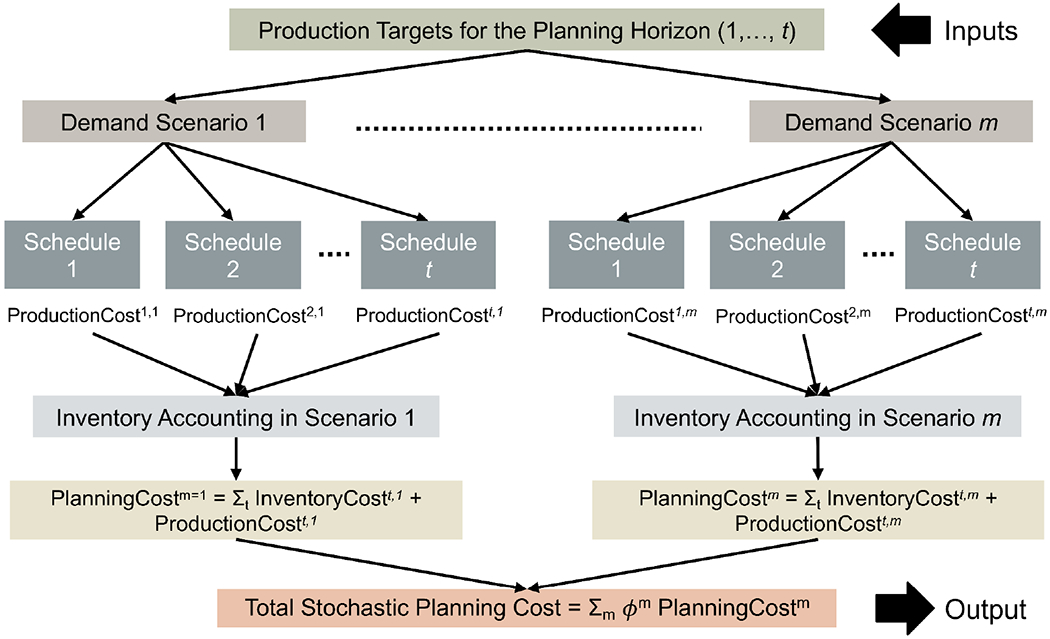
Input-output data collection from the integrated planning and scheduling formulation.
Algorithm 1.
Simulating the Scheduling Level in Stochastic Bi-level Data-Driven Optimization
| Input: (sampling points) |
| for m = 1 → Nm do |
| Require: Demand levels in scenario m |
| Calculate the Day 7 target in scenario m using Equation 10. for i = Day 1, …, Day 7 do |
| Input: Demand(i), Target(i), Inventory(i) |
| if i= Day 1 then |
| Start Inventory(i) = 10 |
| else |
| The start inventory is the ending inventory of the previous day. |
| end if |
| Solve Equation 11 subject to Equations 12–28. |
| Retrieve the optimal objective function value (Production cost). |
| Calculate the violation of Equation 28. |
| Calculate ending inventory using Equation 5. |
| end for |
| Calculate the minimum inventory for each product. |
| for j = 1 → Sp do |
| if min(Inventory Levels(:,j)) < 0 then |
| Final Inventory(:,j) = Inventory Levels(:,j) - min(Inventory Levels(:,j)) |
| else |
| Final Inventory = Inventory Levels |
| end if |
| end for |
| Calculate the inventory cost using Equation 4. Final Inventory = Invs. |
| Calculate the cost of planning at scenario m using Equation 3. |
| Calculate the demand violation using Equation 6. |
| end for |
| Calculate total stochastic cost of planning using Equation 2. |
| Output: total stochastic cost of planning (obj), feasibility violation, demand violation |
Our inputs, which are the decision variables for the leader problem, are the production targets for the products. We only sample for the production targets up to t – 1 periods, as the final production target for each product will be calculated deterministically using Equation 10 to sustain cyclic periods. For every scenario, we first calculate the final production target at the final planning period. Then, the first-day demand, production, and inventory levels are inputted to the scheduling level where Equation 11 is minimized deterministically subject to Equations 12–28. This yields the production cost and the ending inventory for the first planning period in the first scenario. The ending inventory becomes the starting inventory of the next day and this deterministic optimization step is repeated until the final planning period is reached. Once these repeated calculations are completed for the first scenario, the inventories are accounted and the inventory cost is calculated. This final inventory cost and the production cost will be then used to calculate the total cost of planning in the first scenario using Equation 3. We repeat this procedure for the rest of the scenarios and calculate the total stochastic cost of planning as the cumulative total cost of planning weighted with respect to its probability of occurrence (Equation 2). This final value becomes the output for the objective function, accompanied by the feasibility and demand violation information which will be the grey-box constraints for the data-driven optimization step.
2.4. Motivating Example
In this section, we demonstrate the steps for solving integrated planning and scheduling problems using our data-driven optimization approach. For this purpose, we utilize the motivating example presented in Ierapetritou & Floudas (1998) with 1 feed, 3 tasks, 2 intermediates, and 1 product. The state-task network (STN) of the motivating example is provided in Figure 4. The parameters of the problem are summarized in Table 1.
Figure 4:
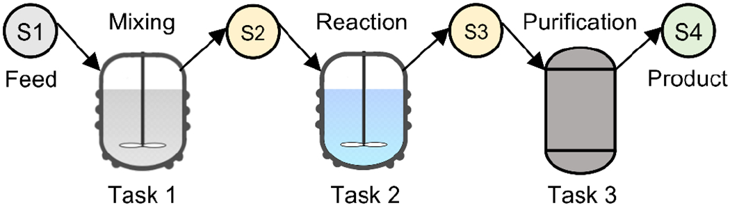
The STN of the motivating example.
Table 1:
Parameters for the motivating example (Example 1).
| Units, j | Task Suitability | ||
|---|---|---|---|
| Mixer | Task 1 | 100 | 4.5 |
| Reactor | Task 2 | 75 | 3.0 |
| Purifier | Task 3 | 50 | 1.5 |
| State, s | Inventory Cost (hs) | ||
|
| |||
| S1 | - | unlimited | unlimited |
| S2 | - | 0 | 100 |
| S3 | - | 0 | 100 |
| S4 (Product) | 10 | 0 | unlimited |
| Fixed Cost | Variable Cost | ||
|
| |||
| Mixing, Purification | 150 | 1 | |
| Reaction | 100 | 0.5 | |
|
| |||
|
| |||
| Number of Event Points (N) | 5 | ||
| Scheduling Time Horizon (H) | 12 | ||
Step 1: Create Scenarios for Uncertain Product Demands
We randomly create 10,000 scenarios with μ = 50, σ = μ/5 = 10, and identify low, medium, and high demand regions as shown on the histogram (Figure 5A). From the overall distribution, the Day 1 demand is sampled for the product and fixed over the studied scenarios. For the rest of the days, random sampling is done within the low, medium, and high demand regions to construct the 9 scenarios (Figure 5B).
Figure 5:

(A) Histogram of the randomly created demand scenarios for Example 1; (B) The sampled demand scenarios for analysis. Note that Day 1 product demand is the same across all scenarios.
Step 2: Define the data-driven system
Once the demand scenarios are generated, the data-driven system is defined. In the motivating example, we are considering a week-long planning period to satisfy the uncertain demand for one product by determining the feasible production targets. This yields 6 decision variables (Day 1-6 production targets for one product) with each day target having lower and upper bounds of [0, 90]. Recall, that the Day 7 target is deterministically defined by Equation 10 to ensure the cyclic formulation, which is not a degree of freedom for the optimization procedure.
After defining the input information, we further define the output information that the data-driven algorithm will process. The output information includes the objective function value and the violations of the grey-box constraints at a given data sample. Our objective is to minimize the total stochastic cost of planning defined by Equation 2. The grey-box constraints are all the equations that contain at least one upper-level decision variable at any level of the bi-level formulation. In this case, these are Equations 6 and 28, where the final number of grey-box constraints depends on the number of products, scenarios, and the planning days considered. Here, we are considering 9 scenarios, 1 product, and 7 planning days, which brings the constraint count to 126 for the data-driven solver to handle. However, it is important to note that as the production targets for Day 1-6 are going to be the same across all scenarios, the violations calculated from Equation 28 will be the same for the first 6 days of the planning period across all scenarios. As a result, this only requires collecting the violation information of the first 6 days of any scenario and the last day targets over the different demand scenarios. This reduces the number of constraints defining the lower-level problem feasibility to 15, making the final constraint count to be 78 for the data-driven optimization process. A summary of the data-driven optimization parameters is provided in Table 2.
Table 2:
Summary of the data-driven problem parameters for the motivating example.
| Number of Decision Variables (All Continuous) | 6 |
| Bounds on Decision Variables | [0,90] |
| Number of Grey-Box Constraints | 78 |
Step 3: Initiate DOMINO at random instances and collect input-output data from the scheduling problem
Once the data-driven system is defined, DOMINO is executed 10 times with random initialization. For the motivating example, we use the NOMAD algorithm within DOMINO. For each sampling point (i.e., candidate production targets for Day 1-6), the scheduling problem is simulated sequentially across the 7 planning days per scenario. To execute this successfully, we follow the recipe given in Algorithm 1.
Step 4: Report the best-found solution
Among the 10 random instances, the run with the minimum objective value is identified and this is reported as the best-found solution. Note that the best-found solution is not guaranteed optimal for the planning level but it is guaranteed feasible (i.e., scheduling level is globally optimal). We assume that the functional forms and the convexity of the objective and the constraints are unknown at the planning level. As a result, we cannot provide theoretical guarantees for global optimality for any solution. This is a disadvantage of the data-driven framework compared to the decomposition-based algorithms, as the latter can provide information on the optimality or duality gaps.
We report the results of the best-found solution for the motivating example in Figure 6. The results show that the production targets and the starting inventories for all scenarios satisfy the changing product demands. In the best-case scenario (Scenario 1), where low demand is expected throughout the planning week, excess production accumulates as inventory towards the end of the planning week. This accumulated inventory decreases with the increasing demand for the product. Specifically, in more demanding scenarios (Scenarios 8 and 9), less inventory accumulates over time, and cumulative unit product from production targets and starting inventories tightly meet the daily demand. Also, the Day 7 production targets and starting inventory levels show that the cyclic nature of the planning problem is preserved where Day 7 production and inventory is greater than or equal to Day 1 starting inventory. In any case, all demand scenarios are satisfied throughout the 7-day planning period and all production targets are optimal for the scheduling problem.
Figure 6:
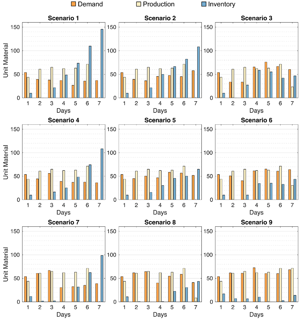
Demand, production, and inventory profiles for the desired product over all studied scenarios in the motivating example.
We also analyze the effect of random initialization on the consistency of our data-driven approach. For every scenario, we plot the demand, production, and starting inventory profiles with error bars showing the minimum and maximum deviation from the best-found solution per planning day (Figure S1). These profiles indicate that DOMINO-NOMAD is very consistent in finding the same solution with the final total stochastic cost of planning having ± 0.1039 standard error across the 10 random runs. Only a slight variability is observed in Day 6 results over all scenarios where the positive and negative deviation does not exceed 27 units of material. Like in the best-found solution, all solutions obtained from the random initialization of NOMAD were also guaranteed feasible with globally optimal schedules. Analysis of other computational case studies and the effects of data-driven solver choice, as well as the characterization of planning and scheduling formulation complexities, are provided in detail in the following Section.
3. Computational Case Studies
In addition to the motivating example, we demonstrate the applicability of our approach on two other computational case studies with scheduling examples obtained from Kondili (1987) and Ierapetritou & Floudas (1998) (Figures 7–8). Example 2 considers the production of 2 products through 9 states using 8 tasks in 4 units, and Example 3 considers the production of 4 products through 13 states using 8 tasks in 6 units. Example 2 yields a data-driven optimization problem with 12 decision variables with lower and upper bounds of [0, 90] and 156 grey-box constraints, and Example 3 yields a data-driven optimization problem with 24 decision variables with lower and upper bounds of [0, 1000] and 312 grey-box constraints. The parameters for modeling these examples are provided in Supplementary Tables S1–S2.
Figure 7:

STN of Example 2.
Figure 8:

STN of Example 3.
The demand profile for the computational study is randomly created following the steps provided in Section 2.4 with Example 2 having a mean distribution of μ = 50 with standard deviation σ = 10, and Example 3 having a mean distribution of μ = 500 with standard deviation σ = 100. The histogram of the randomly created demand scenarios and the plot of demand levels across planning days for the selected scenarios are provided in the Supplementary Figures S2–S4.
For each case study, we use the DOMINO algorithm with a different data-driven optimization solver to test the effect of solver choice in these bi-level mixed-integer formulations. We test the solvers listed in Table 3 to capture the differences between model-based and sample-based approaches, as well as local and global solution strategies. A portion of these solvers was also benchmarked in our previous study (Beykal et al., 2020a) for solving single-follower bi-level optimization problems where they have shown superior performance in finding the known optimal solution of many different types of bi-level programming problems.
Table 3:
Data-driven optimization solvers tested as a part of DOMINO.
| Solver Name | Type | Optimization Strategy | Initialization Type | Reference |
|---|---|---|---|---|
| NOMAD | Sample-Based | Local | Single Point | (Audet & Dennis Jr, 2009) |
| ISRES | Sample-Based | Global | Single Point | (Runarsson & Yao, 2005) |
| COBYLA | Model-Based | Local | Single Point | (Powell, 1994) |
| EGO | Model-Based | Global | Latin Hypercube | (Jones et al., 1998) |
| ARGONAUT | Model-Based | Global | Latin Hypercube | (Boukouvala & Floudas, 2017) |
Furthermore, we modify the objective functions of the planning and scheduling levels to observe the effects of nonlinear formulations in the solver performance and optimization results. We consider an NLP formulation for the upper-level objective (Equation 29) and a QP formulation for the lower-level objective (Equation 30). Note that only the variable cost terms in each objective function are modified into a nonlinear form since the fixed cost is going to be constant throughout. We introduce a number of parameters in these formulations to achieve balanced and representative profiles of variable costs. The parameters of the new objective functions are heuristically determined by studying possible cost profiles within the lower and upper bounds of production targets and capacities of the units in the scheduling layer. For example, to prevent variable cost from overshooting quickly with the increasing amount of material undertook in tasks and units, we introduce a multiplier γ in the scheduling level objective function. In Examples 1 and 2, we use γ = 0.05 whereas, for Example 3, we use γ = 0.005 due to the higher amount of material processed in the scheduling layer of the latter computational study. These modifications in the objective functions help us to have a more realistic assessment of the variable cost in both layers of the integrated planning and scheduling problems, as linear formulations are approximations of the true nonlinear behavior. It also allows us to demonstrate one of the biggest advantages of the framework over deterministic and exact algorithms, which is the ability to handle high-dimensional and highly nonlinear bi-level optimization problems with a feasibility guarantee. The profiles and parameters of the cubic and quadratic terms in Equations 29 and 30 are provided in Supplementary Figures S5 and S6.
| (29) |
| (30) |
Finally, we test the effect of the scheduling level complexity on our data-driven optimization strategy when the number of event points is increased. The increasing number of event points have a direct impact on the complexity of the scheduling problem as it also increases the number of equations, binary and continuous variables in the formulation. Previous works have focused on determining the optimal number of event points to address this key issue (Janak & Floudas, 2008; Li & Floudas, 2010). Our goal is to test the boundaries of the proposed data-driven methodology and demonstrate the impact of the lower-level problem on the overall bi-level optimization performance. Hence, we study the following lower-level complexities for each case study:
All computational case studies are executed on a High-Performance Computing machine at Texas A&M High-Performance Research Computing facility using Ada IBM/Lenovo Intel Xeon E5-2670 v2 (Ivy Bridge-EP) HPC Cluster. When DOMINO is integrated with COBYLA, ISRES, EGO, and NOMAD algorithms, these case studies are executed using 1 node (1 core per node with 64 GB RAM) on the supercomputer. In cases where DOMINO is integrated with the ARGONAUT algorithm, then these cases are executed as a parallel job, using 1 node (20 cores per node with 64 GB RAM) on the supercomputer. The scheduling levels of all formulations are solved using CPLEX 12.8.0.0.
4. Results and Discussion
The results of the best-found solution by each solver are presented in Table 5 and the overall performance of each solver across the random repeated runs are shown in Figure S7. For the LP-MILP formulation of Example 1, the best-found solution is identified by NOMAD and all random runs are reported to be guaranteed feasible with scheduling levels solved to global optimality. The feasible demand, production, and inventory profiles corresponding to the best solution were presented in the motivating example in Figure 6 and the variability in these profiles across the random runs was presented in Supplementary Figure S1. The results indicate that NOMAD shows superior performance in finding the lower total stochastic cost of planning for Example 1. Although ARGONAUT converges to a slightly higher objective function value, the variability in the total stochastic cost value among the random runs is lower compared to NOMAD where all repeated runs are guaranteed feasible. Among the other tested data-driven optimizers, COBYLA reported the second-best objective function value, however, one of the repeated random runs converged to an infeasible solution. Similarly, EGO reported 2 infeasible solutions among the 10 tested random runs, and the best-found solution by this algorithm yielded the highest total stochastic cost of planning compared to other solvers. Furthermore, we observe that the ISRES algorithm did not report any feasible solutions within the 144 h of wall time set on the HPC machine and hence, excluded from Figure S7. Although ISRES was previously shown to have good performance over single-follower LP-MILP bi-level benchmark problems with 10-30 upper-level decision variables (Beykal et al., 2020a), we observe that increasing number of constraints in the integrated planning and scheduling problems and the longer simulation time required to collect one sample from the stochastic analysis adversely affected the solver performance.
Table 5:
The best-found solutions for the integrated planning and scheduling case studies using DOMINO with various data-driven optimization solvers. The scheduling levels for Example 1 and 2 are solved with 5 event points whereas for Example 3, 6 event points are used. Standard deviation is calculated with the scaled objective function values reported below. The bold values reflect the best-performing solver among the tested.
| NOMAD | COBYLA | ARGONAUT | EGO | ISRES | |
|---|---|---|---|---|---|
| Example 1 | |||||
|
| |||||
| LP-MILP/1000 | 7.11 | 7.42 | 7.45 | 8.16 | - |
| Infeasible Runs (Out of 10) | 0 | 1 | 0 | 2 | 10 |
| Std. Dev. | 0.33 | 0.78* | 0.28 | 0.73* | - |
| Tot. No. Samples | 1508 | 187 | 3028 | 97 | - |
| NLP-MIQP/1000 | 6.20 | 6.41 | 6.29 | 6.46 | 6.66 |
| Infeasible Runs | 0 | 1 | 0 | 2 | 9 |
| Std. Dev. | 0.04 | 0.26* | 0.06 | 0.2 | 0* |
| Tot. No. Samples | 658 | 131 | 4258 | 106 | 8507 |
|
| |||||
| Example 2 | |||||
|
| |||||
| LP-MILP/1000 | 13.52 | 15.03 | 14.49 | 15.32 | - |
| Infeasible Runs | 0 | 9 | 0 | 3 | 10 |
| Std. Dev. | 0.28 | 0* | 0.65 | 0.9* | - |
| Tot. No. Samples | 2972 | 396 | 2912 | 210 | - |
| NLP-MIQP/1000 | 12.21 | - | 12.33 | 12.55 | - |
| Infeasible Runs | 0 | 10 | 0 | 3 | 10 |
| Std. Dev. | 0.09 | - | 0.1 | 0.23 | - |
| Tot. No. Samples | 2527 | - | 2358 | 127 | - |
|
| |||||
| Example 3 | |||||
|
| |||||
| LP-MILP/1000 | 102.08 | 109.46 | 112.73 | 120.33 | 130.20 |
| Infeasible Runs | 0 | 3 | 0 | 0 | 4 |
| Std. Dev. | 0.92 | 10.66* | 3.4 | 3.21 | 4.26* |
| Tot. No. Samples | 9572 | 1015 | 1165 | 376 | 7950 |
| NLP-MIQP/1000 | 224.69 | 224.94 | 233.12 | 241.15 | 277.39 |
| Infeasible Runs | 0 | 4 | 0 | 0 | 7 |
| Std. Dev. | 0.2 | 27.65* | 5.44 | 7.84 | 8.24* |
| Tot. No. Samples | 9426 | 4097 | 1169 | 288 | 6409 |
Standard deviation calculation excludes infeasible runs.
Furthermore, the results of the NLP-MIQP formulation of Example 1 (profiles provided in Figure S8) show that the total stochastic cost of planning at the best-found solution is slightly lower for all algorithms compared to the LP-MILP formulation whereas the number of infeasible solutions encountered by each algorithm is the same, with the best-found objective function value identified by NOMAD. Different than the linear formulation, we observe that ARGONAUT surpasses COBYLA in finding the second-best solution in the nonlinear case. This superior performance is expected as ARGONAUT can handle nonlinear formulations and perform global optimization on the surrogate forms to retrieve the best solution. On the other hand, COBYLA relies on local linear approximations for all encountered problems which do not capture the nonlinear behavior in the objective functions of both layers of the modified stochastic integrated planning and scheduling formulation. We also observe that although ISRES was unable to find a feasible solution within the provided time limits in the LP-MILP case, it identified a feasible solution for one of the random runs in the NLP-MIQP case. Nonetheless, we observe that our multi-follower strategy combined with DOMINO-NOMAD or DOMINO-ARGONAUT surpasses other algorithms and finds consistent guaranteed feasible solutions for the nonlinear BMF-MIP formulations.
For the LP-MILP formulation of Example 2, the best-found solution is again identified by DOMINO-NOMAD where the feasible demand, production, and inventory profiles are presented in Figures 9 and 10. The results are consistent with the motivating example where all demand scenarios are satisfied, the lower-level scheduling is solved to global optimality, and the best-found solution is guaranteed feasible for the stochastic integrated planning and scheduling problem. Similarly, we observe that excess inventory is accumulated for easier scenarios where demand levels tend to be lower within the 7-day planning period. However, with increasing demand, less inventory is accumulated, and the production targets tightly meet the more demanding scenarios for both products. This also has an effect on satisfying the cyclic consideration of the planning period. In low and medium demand scenarios, as more inventory is accumulated towards the end of the planning week, it is easier to satisfy the continuity of the production planning in the following planning period. In more challenging scenarios, as the production targets tightly meet the demand and less inventory is generated, sustaining the continuity in the following planning week is harder to achieve. Even so, the last day production and starting inventory always satisfy the Day 7 demand for both products and is enough to provide the Day 1 starting inventory of the next planning period. The variability in the best-found demand, production, and inventory profiles for both products across the random runs was also similar to Example 1, where a slightly more variability is observed in Product 2 profiles across the entire planning period (Figures S9 and S10). This is an expected result as there are twice as many decision variables and grey-box constraints for the data-driven solvers to handle in Example 2, which is a significant increase from the previous case study.
Figure 9:

Demand, production, and inventory profiles for Product 1 of Example 2 with the LP-MILP formulation.
Figure 10:

Demand, production, and inventory profiles for Product 2 of Example 2 with the LP-MILP formulation.
Similar to the trends observed in the results of Example 1, NOMAD also outperforms other data-driven optimizers in solving the NLP-MIQP formulation of Example 2. As shown in Table 5 and Figure S7, NOMAD consistently finds the superior feasible solution where all repeated runs are guaranteed feasible. The corresponding demand, production, and inventory profiles are provided in Supplementary Figures S11–S12. On the other hand, the performance of COBYLA deteriorates in this case study with the increasing number of variables and constraints. We observe that 9 out of the 10 runs reported infeasible solutions for the LP-MILP formulation whereas all runs were infeasible for the nonlinear case. The deteriorating performance of COBYLA in the nonlinear formulation is somewhat expected since this algorithm builds local linear surrogate forms that do not fully capture the nonlinear behavior of the underlying formulation. Also, the inferior performance in the LP-MILP case indicates that the increasing number of variables and constraints, combined with the multi-follower nature of this study, as well as the stochastic analysis, created a much more challenging optimization problem for COBYLA to retrieve a feasible solution, as this algorithm was previously shown to have good performance in similar dimensional benchmark problems for single-follower LP-MILP and NLP-MIQP bi-level formulations (Beykal et al., 2020a). Furthermore, we observe that ISRES is unable to report any feasible solutions for Example 2 and the number of infeasible runs also increases for EGO. However, ARGONAUT consistently provides guaranteed feasible solutions even with the increasing number of variables and constraints in both levels and planning formulations and performs comparable to NOMAD both in terms of consistency, feasibility, the total number of samples collected, and the final objective function value at the best-found solution.
Furthermore, the results of the most challenging case study, Example 3, also tell a similar story to what we observed in the previous examples. The demand, production, and inventory profiles for the first product are provided in Figure 11 with the rest of the profiles for the other products, and their variability across the random runs are provided in Supplementary Figures S13–S20. The results show that DOMINO-NOMAD consistently identifies the best solution for both LP-MILP and NLP-MIQP formulations of Example 3 with all demand scenarios are satisfied, all schedules are globally optimal, and the best-found solution is guaranteed feasible. This is a significant result, especially when the nonlinear formulation is considered, as DOMINO handles this integrated bi-level problem that contains several hundred constraints, binary and continuous variables in the scheduling subproblems easily. Different than the previous observations, we see that NOMAD collects significantly more samples compared to the other algorithms to converge to the best solution (Table 5 and Figure S7). Yet, NOMAD is very consistent in identifying the better objective value with a very low standard deviation. We also observe that EGO’s performance is improved in Example 3 where all executed runs are feasible for both LP-MILP and NLP-MIQP formulation. However, the final objective function of the best-found solution by EGO is marginally higher than NOMAD’s best-reported solution. Unlike Example 2, we further observe that COBYLA and ISRES can identify more feasible solutions for Example 3. This shows that even in high-dimensional cases DOMINO can recover the guaranteed feasible solution through its data-driven optimization capabilities.
Figure 11:

Demand, production, and inventory profiles for Product 1 of Example 3 with the NLP-MIQP formulation.
Finally, we assess the effect of the scheduling level complexity on the optimization performance. For this purpose, we only analyze NOMAD which is the best performing algorithm for solving the BMF-MIP formulations of integrated planning and scheduling problems. As shown in Figure 12, the best-found total stochastic cost of planning across the varying number of event points in the scheduling formulation is nearly the same for all examples with the exception in Example 3 where a drop in the total cost is when the number of event points is increased to 6. However, the computational expense of retrieving the best solution significantly increases with increasing lower-level complexity. In Example 1, it took on average 26 seconds to collect 1 sample with a 5-event point scheduling formulation whereas this increased to 56 seconds with 10 event points. In the case of Example 2, the computational time required to collect 1 sample on average was about 28 seconds with 5 event points whereas this increased to 2279 seconds with 10 event points. Likewise, the results for Example 3 in Figure 12C show that increasing scheduling level complexity increases the total computational expense. Approximately 27 seconds on average was spent to collect a single sample with 5 events points whereas this increased to 121 seconds per sample with 10 event points. Even though the lower-level problem is deterministically solved to global optimality over every planning horizon and scenario, more event points lead to a larger optimization problem where CPLEX is taking a longer time to find the optimal solution per sample. Naturally, this computational expense accumulates over multiple planning periods, scenarios, and many collected samples which increases the total processing time.
Figure 12:

The effect of the MILP scheduling level complexity on the data-driven optimization: (A) Example 1; (B) Example 2; (C) Example 3 with DOMINO-NOMAD. Bar plot showing the minimum total stochastic cost of planning for the best-found solution whereas the line plot showing the computational time spent across the increasing number of event points in the scheduling formulation.
We also report the average total number of samples across the different number of event points studied in each example in Table 6. We observe that the total number of samples across the varying number of event points is relatively stable for Example 1. Thus, the increasing computational expense trend seen in Figure 12A is attributed to the increasing cost of sample collection with more event points in the scheduling formulation. However, in Example 2, we see a drastic decrease in the total number of samples collected when we study a higher number of event points in the scheduling level. As the sample collection gets very exhaustive with the increasing number of event points, the data-driven algorithm was not able to collect all the necessary samples, and the runs are terminated by hitting the wall time limit on the supercomputer (Figure 12B). Likewise in Example 3, we are also seeing a decreasing number of sample collections with the increasing number of event points, where in formulations with 8-10 event points, all runs hit the computational time limit. Although in this case, the collection of a single sample is not as exhaustive as in Example 2, this problem is relatively harder to solve from a data-driven optimization perspective due to the high number of decision variables and grey-box constraints that the solver needs to handle. As a result, NOMAD requires more samples compared to previous case studies and this is not achieved when the lower-level problem is also computationally demanding within the preset wall time limits. Here, the parallelization of the framework will further improve computational efficiency by solving every scenario and scheduling subproblems as independent optimization problems and can overcome the aforementioned difficulties with high-dimensional case studies. Nonetheless, our data-driven approach can find guaranteed feasible solutions for the integrated problem, even when the scheduling layer has thousands of constraints and a few hundred continuous and binary variables.
Table 6:
The average total number of samples collected for the computational case studies across varying number of event points.
| Number of Event Points | 5 | 6 | 7 | 8 | 9 | 10 |
|---|---|---|---|---|---|---|
| Example 1 | 1288 | 1217 | 1141 | 1171 | 1083 | 1150 |
| Example 2 | 2873 | 3486 | 3226 | 1358 | 519 | 225 |
| Example 3 | 13703* | 10811 | 9445 | 8212 | 5657 | 4207 |
Average calculation excludes infeasible runs.
5. Conclusions
In this work, we study the simultaneous modeling and optimization of planning and scheduling problems under demand uncertainty using mixed-integer bi-level multi-follower programming and data-driven optimization. We extend the DOMINO algorithm, which is designed to solve single-leader single-follower bi-level problems, to solve single-leader multi-follower stochastic problems, and use various product demand scenarios to perform stochastic analysis on the integrated problem. The input-output data for the data-driven optimization step is collected by sampling the production targets at the planning level and solving the scheduling problems to global optimality for every planning period and scenario. We explore a plethora of effects on the bi-level multi-follower optimization performance of DOMINO including, linear and nonlinear cost functions at both levels, the choice of data-driven solver embedded in DOMINO, and the scheduling level complexity on the overall optimization performance. Our results on single and multi-product case studies show that our data-driven bi-level multi-follower approach can identify guaranteed feasible solutions for the integrated planning and scheduling formulations, even with highly complex scheduling levels that contain thousands of constraints and several hundred continuous and binary variables.
Supplementary Material
Table 4:
Scheduling formulation complexity of the tested problems.
| Event Points | Bin. Variables | Cont. Variables | Constraints | |
|---|---|---|---|---|
| Example 1 | 5-10 | 45-90 | 95-190 | 203-423 |
| Example 2 | 5-10 | 160-320 | 285-570 | 712-1522 |
| Example 3 | 5-10 | 240-480 | 385-770 | 732-1552 |
Notation.
| Indices | |
| i ∈ I | tasks |
| j ∈ I | units |
| m ∈ Nm | scenarios |
| n ∈ N | event points representing the beginning of a task |
| s ∈ S | states |
| t ∈ T | planning period |
| Sets | |
| Ij | tasks that can be produced in unit j |
| Is | tasks that can process state s (either produce or consume) |
| Ji | units that are suitable for performing task i |
| Sp | products |
| Parameters | |
| δ | parameter in the cubic inventory cost function |
| ϵ | parameter in the cubic inventory cost function |
| η | parameter in the cubic inventory cost function |
| θ | parameter in the cubic inventory cost function |
| γ | multiplier for the quadratic variable cost term |
| hs | inventory unit cost of state s |
| H | scheduling time horizon in hours |
| αi,j | constant term of processing time of task i at unit j |
| βi,j | variable term of processing time of task i at unit j expressing the time required by the unit to process one unit of material performing task i |
| proportion of state s produced from task i, | |
| proportion of state s consumed from task i, | |
| initial amount of state s in planning period t | |
| maximum available storage capacity for state s in planning period t | |
| mean processing time of task i in unit j | |
| minimum processing time of task i in unit j | |
| maximum processing time of task i in unit j | |
| minimum amount of material processed by task i required to start operating unit j | |
| maximum amount of material processed by task i required to start operating unit j | |
| FixCosti | fixed cost of task i |
| VarCosti | variable cost of task i |
| Positive Variables | |
| demand of product s in planning period t in scenario m | |
| inventory level of state s at the end of planning period t in scenario m | |
| production target of state s in the planning period t | |
| amount of material undertaking task i in unit j at event point n in the planning period t in scenario m | |
| amount of state s at event point n in planning period t in scenario m | |
| time that task i starts in unit j at event point n in planning period t in scenario m | |
| time that task i finishes in unit j while it starts at event point n in planning period t in scenario m | |
| Binary Variables | |
| binary variables that assign whether or not task i in unit j start at event point n in the planning period t in scenario m | |
| Variables | |
| ProductionCostt,m | scheduling level objective function value at the end of planning period t in scenario m |
| InventoryCostt,m | inventory cost at the end of planning period t in scenario m |
| Total Cost of Planningm | total cost of planning in scenario m |
Highlights.
We present a data-driven algorithm for the solution of integrated planning and scheduling problems under uncertainty.
The proposed algorithm is based upon the recently developed DOMINO framework for the solution of single-follower bi-level problems, which is here extended for the solution of bilevel multi-follower stochastic optimization problems.
Computational studies to show the applicability of the proposed approach are presented through the solution of three planning and scheduling case studies.
Acknowledgments
This work was supported by the National Institutes of Health [NIH P42-ES027704], the National Science Foundation (Grant no. 1739977 [INFEWS]), RAPID SYNOPSIS Project (DE-EE0007888-09-03) and DOE-CESMII Energy Efficient Operation of Air Separation Processes Project (DE-EE0007613, 4550 G WA324). The authors also gratefully acknowledge financial support from Texas A&M University, Texas A&M Energy Institute, and the University of Connecticut. Portions of this research were conducted with the advanced computing resources provided by Texas A&M High-Performance Research Computing. The manuscript contents are solely the responsibility of the grantee and do not necessarily represent the official views of the NIH. Further, NIH does not endorse the purchase of any commercial products or services mentioned in the publication.
Footnotes
Publisher's Disclaimer: This is a PDF file of an unedited manuscript that has been accepted for publication. As a service to our customers we are providing this early version of the manuscript. The manuscript will undergo copyediting, typesetting, and review of the resulting proof before it is published in its final form. Please note that during the production process errors may be discovered which could affect the content, and all legal disclaimers that apply to the journal pertain.
Declaration of Competing Interest
The authors declare that they have no known competing financial interests or personal relationships that could have appeared to influence the work reported in this paper.
References
- Audet C, & Dennis JE Jr (2009). A progressive barrier for derivative-free nonlinear programming. SIAM Journal on Optimization, 20, 445–472. [Google Scholar]
- Avraamidou S, Beykal B, Pistikopoulos IPE, & Pistikopoulos EN (2018). A hierarchical food-energy-water nexus (few-n) decision-making approach for land use optimization. In Computer Aided Chemical Engineering (pp. 1885–1890). Elsevier; volume 44. [DOI] [PMC free article] [PubMed] [Google Scholar]
- Avraamidou S, & Pistikopoulos EN (2017). A multiparametric mixed-integer bi-level optimization strategy for supply chain planning under demand uncertainty. IFAC-PapersOnLine, 50, 10178–10183. 20th IFAC World Congress. [Google Scholar]
- Avraamidou S, & Pistikopoulos EN (2018). A novel algorithm for the global solution of mixed-integer bi-level multi-follower problems and its application to planning scheduling integration. In 2018 European Control Conference (ECC) (pp. 1056–1061). doi: 10.23919/ECC.2018.8550351. [DOI] [Google Scholar]
- Avraamidou S, & Pistikopoulos EN (2019a). B-POP: Bi-level parametric optimization toolbox. Computers & Chemical Engineering, 122, 193–202. [DOI] [PMC free article] [PubMed] [Google Scholar]
- Avraamidou S, & Pistikopoulos EN (2019b). A bi-level formulation and solution method for the integration of process design and scheduling. In Computer Aided Chemical Engineering (pp. 17–22). Elsevier; volume 47. [Google Scholar]
- Avraamidou S, & Pistikopoulos EN (2019c). A multi-parametric optimization approach for bilevel mixed-integer linear and quadratic programming problems. Computers & Chemical Engineering, 125, 98–113. [Google Scholar]
- Beykal B, Avraamidou S, & Pistikopoulos EN (2021). Bi-level mixed-integer data-driven optimization of integrated planning and scheduling problems. In Computer Aided Chemical Engineering (pp. 1707–1713). Elsevier; volume 50. [DOI] [PMC free article] [PubMed] [Google Scholar]
- Beykal B, Avraamidou S, Pistikopoulos IPE, Onel M, & Pistikopoulos EN (2020a). DOMINO: Data-driven optimization of bi-level mixed-integer nonlinear problems. Journal of Global Optimization, 78, 1–36. [DOI] [PMC free article] [PubMed] [Google Scholar]
- Beykal B, Boukouvala F, Floudas CA, & Pistikopoulos EN (2018a). Optimal design of energy systems using constrained grey-box multi-objective optimization. Computers & Chemical engineering, 116, 488–502. [DOI] [PMC free article] [PubMed] [Google Scholar]
- Beykal B, Boukouvala F, Floudas CA, Sorek N, Zalavadia H, & Gildin E (2018b). Global optimization of grey-box computational systems using surrogate functions and application to highly constrained oil-field operations. Computers & Chemical Engineering , 114, 99–110. [Google Scholar]
- Beykal B, Onel M, Onel O, & Pistikopoulos EN (2020b). A data-driven optimization algorithm for differential algebraic equations with numerical infeasibilities. AIChE Journal, 66, e16657. [DOI] [PMC free article] [PubMed] [Google Scholar]
- Bi K, Beykal B, Avraamidou S, Pappas I, Pistikopoulos EN, & Qiu T (2020). Integrated modeling of transfer learning and intelligent heuristic optimization for a steam cracking process. Industrial & Engineering Chemistry Research, 59, 16357–16367. [DOI] [PMC free article] [PubMed] [Google Scholar]
- Boukouvala F, & Floudas CA (2017). ARGONAUT: Algorithms for global optimization of constrained grey-box computational problems. Optimization Letters, 11, 895–913. [Google Scholar]
- Calvete HI, & Galé C (2007). Linear bilevel multi-follower programming with independent followers. Journal of Global Optimization, 39, 409–417. [Google Scholar]
- Chu Y, You F, Wassick JM, & Agarwal A (2015). Integrated planning and scheduling under production uncertainties: Bi-level model formulation and hybrid solution method. Computers & Chemical Engineering, 72 , 255–272. [Google Scholar]
- Cozad A, Sahinidis NV, & Miller DC (2014). Learning surrogate models for simulation-based optimization. AIChE Journal, 60, 2211–2227. [Google Scholar]
- Dias LS, & Ierapetritou MG (2019). Data-driven feasibility analysis for the integration of planning and scheduling problems. Optimization and Engineering, 20, 1029–1066. [Google Scholar]
- Dogan ME, & Grossmann IE (2006). A decomposition method for the simultaneous planning and scheduling of single-stage continuous multiproduct plants. Industrial & engineering chemistry research, 45, 299–315. [Google Scholar]
- Faísca NP, Saraiva PM, Rustem B, & Pistikopoulos EN (2009). A multi-parametric programming approach for multilevel hierarchical and decentralised optimisation problems. Computational management science, 6, 377–397. [Google Scholar]
- Grossmann I (2005). Enterprise-wide optimization: A new frontier in process systems engineering. AIChE Journal, 51, 1846–1857. [Google Scholar]
- Grossmann IE (2012). Advances in mathematical programming models for enterprise-wide optimization. Computers & Chemical Engineering, 47, 2–18. [Google Scholar]
- Gümüş ZH, & Floudas CA (2005). Global optimization of mixed-integer bilevel programming problems. Computational Management Science, 2, 181–212. [Google Scholar]
- Ierapetritou MG, & Floudas CA (1998). Effective continuous-time formulation for short-term scheduling. 1. multipurpose batch processes. Industrial & Engineering Chemistry Research, 37, 4341–4359. [Google Scholar]
- Janak SL, & Floudas CA (2008). Improving unit-specific event based continuous-time approaches for batch processes: Integrality gap and task splitting. Computers & Chemical Engineering, 32, 913–955. [Google Scholar]
- Jones DR, Schonlau M, & Welch WJ (1998). Efficient global optimization of expensive black-box functions. Journal of Global optimization, 13, 455–492. [Google Scholar]
- Katz J, Pappas I, Avraamidou S, & Pistikopoulos EN (2020). Integrating deep learning models and multiparametric programming. Computers & Chemical Engineering, 136, 106801. [Google Scholar]
- Kim SH, & Boukouvala F (2020). Surrogate-based optimization for mixed-integer nonlinear problems. Computers & Chemical Engineering, 140, 106847. [Google Scholar]
- Kleniati P-M, & Adjiman CS (2015). A generalization of the branch-and-sandwich algorithm: from continuous to mixed-integer nonlinear bilevel problems. Computers & Chemical Engineering, 72 , 373–386. [Google Scholar]
- Kondili E (1987). Optimal scheduling of batch chemical processes. Ph.D. thesis Imperial College London (University of London). [Google Scholar]
- Li J, & Floudas CA (2010). Optimal event point determination for short-term scheduling of multipurpose batch plants via unit-specific event-based continuous-time approaches. Industrial & Engineering Chemistry Research, 49, 7446–7469. [Google Scholar]
- Li Z, & Ierapetritou MG (2009). Integrated production planning and scheduling using a decomposition framework. Chemical Engineering Science, 64, 3585–3597. [Google Scholar]
- Lu J, Shi C, & Zhang G (2006). On bilevel multi-follower decision making: General framework and solutions. Information Sciences, 176, 1607–1627. [Google Scholar]
- Lu J, Shi C, Zhang G, & Dillon T (2007). Model and extended kuhn–tucker approach for bilevel multi-follower decision making in a referential-uncooperative situation. Journal of Global Optimization, 38, 597–608. [Google Scholar]
- Maravelias CT, & Sung C (2009). Integration of production planning and scheduling: Overview, challenges and opportunities. Computers & Chemical Engineering, 33, 1919–1930. [Google Scholar]
- Mistry M, Letsios D, Krennrich G, Lee RM, & Misener R (2020). Mixed-integer convex nonlinear optimization with gradient-boosted trees embedded. INFORMS Journal on Computing, . [Google Scholar]
- Mitsos A (2010). Global solution of nonlinear mixed-integer bilevel programs. Journal of Global Optimization, 47, 557–582. [Google Scholar]
- Papageorgiou LG (2009). Supply chain optimisation for the process industries: Advances and opportunities. Computers & Chemical Engineering, 33, 1931–1938. [Google Scholar]
- Powell MJ (1994). A direct search optimization method that models the objective and constraint functions by linear interpolation. In Advances in optimization and numerical analysis (pp. 51–67). Springer. [Google Scholar]
- Runarsson TP, & Yao X (2005). Search biases in constrained evolutionary optimization. IEEE Transactions on Systems, Man, and Cybernetics, Part C (Applications and Reviews), 35, 233–243. [Google Scholar]
- Saharidis GK, & Ierapetritou MG (2009). Resolution method for mixed integer bi-level linear problems based on decomposition technique. Journal of Global Optimization, 44, 29–51. [Google Scholar]
- Schweidtmann AM, Clayton AD, Holmes N, Bradford E, Bourne RA, & Lapkin AA (2018). Machine learning meets continuous flow chemistry: Automated optimization towards the pareto front of multiple objectives. Chemical Engineering Journal, 352, 277–282. [Google Scholar]
- Shi C, Zhou H, Lu J, Zhang G, & Zhang Z (2007). The kth-best approach for linear bilevel multifollower programming with partial shared variables among followers. Applied mathematics and computation, 188, 1686–1698. [Google Scholar]
- Sinha A, Malo P, Frantsev A, & Deb K (2014). Finding optimal strategies in a multi-period multi-leader–follower stackelberg game using an evolutionary algorithm. Computers & Operations Research, 41, 374–385. [Google Scholar]
- Sung C, & Maravelias CT (2007). An attainable region approach for production planning of multiproduct processes. AIChE Journal, 53, 1298–1315. [Google Scholar]
- Sung C, & Maravelias CT (2009). A projection-based method for production planning of multiproduct facilities. AIChE journal, 55, 2614–2630. [Google Scholar]
Associated Data
This section collects any data citations, data availability statements, or supplementary materials included in this article.