Measurement of the Translational Diffusion Coefficient and Hydrodynamic Radius of Proteins by Dynamic Light Scattering

Abstract

Diffusion is a fundamental process in biological systems that governs the molecular collisions driving biochemical reactions and membrane and transport. Measurement of the diffusion coefficient and application of the Stokes-Einstein equation produces the hydrodynamic radius, which is a commonly used gauge of particle size. Additionally, measurement of the diffusion coefficient and the sedimentation coefficient, and application of the Svedberg equation, yields the molecular weight, which is particularly useful in the characterization of very large macromolecules. Dynamic light scattering (DLS) is the most common method to measure the diffusion coefficient of macromolecules. We describe a procedure to perform DLS measurements on monomeric bovine serum albumin (BSA) purified by size-exclusion chromatography using the Zetasizer Nano S particle size analyzer. We compare several analytical methods in existing software programs to estimate the diffusion coefficient of BSA (extrapolated to water at 20°C at infinite dilution, $D_{20,w}^0$) and describe a statistical method to obtain 95% confidence limits of the precision of the estimates. We compare $D_{20,w}^0$ estimates to literature values obtained by diffusiometry, sedimentation velocity analytical ultracentrifugation, and other DLS instruments. The method of cumulant analysis in the program SEDFIT (www.analyticalultracentrifugation.com) produced the most precise estimate, $D_{20,w}^0$ 6.06 ± 0.07 F (1 F = 10^-7 cm² s^-1), which was within the range of estimates obtained by diffusiometry or sedimentation velocity. This protocol is useful for DLS method validation and quality control.

Background

Diffusion is a process whereby solute concentration differences spontaneously decrease toward a state of homogeneity. It is a fundamental process in biological systems that governs the molecular collisions that drive biochemical reactions and intracellular transport (Berg, 1983). Strictly speaking, this process is called translational diffusion in contrast to the rotational diffusion of particles. An empirical law describing one-dimensional diffusion was described by Fick in the 19^th century, which states that the rate of flow of particles is proportional to the concentration gradient at a given position. The proportionality constant is called the diffusion coefficient, D.

A molecular interpretation of diffusion was made by Einstein in a series of papers beginning in 1905 (Einstein, 1926 [English translation first]). Einstein proposed that solute particles are subjected to forces due to collisions with solvent particles that are in random, Brownian motion due to thermal energy. A particle that is accelerated by a collisional force experiences a resistive force that is proportional to the particle velocity. The proportionality constant, called the frictional coefficient, f, is a function of the size and shape of the particle. Einstein’s law of diffusion is

where k is Boltzmann’s constant and T is the absolute temperature. This equation is fundamental to the understanding of the hydrodynamic properties of macromolecules. It is important to note that it is restricted to a two-component system, e.g., a solute molecule and solvent water, in dilute solution. In a three-component system (e.g., a macromolecule, a low molecular weight electrolyte, and water), there are four diffusion coefficients, one each that components 2 and 3 would have in the absence of the other and two cross-diffusion coefficients (Tanford, 1961). In most dynamic light scattering (DLS) studies, measurements are made under so-called pseudobinary conditions, namely at low macromolecular concentration in a solution that contains an electrolyte at sufficiently high concentration to screen the charge of the macromolecule. Under these conditions, cross-diffusion terms are considered negligible.

For a spherical particle with radius R, Stokes’ law is

where η is the solvent viscosity. Combined with the Einstein equation, the radius of a spherical particle can be calculated if its diffusion coefficient is measured in a solution with known temperature and viscosity

For a particle with arbitrary shape, the hydrodynamic radius, R_h (also called the Stokes radius), can be calculated using the Stokes-Einstein equation

The hydrodynamic radius of a particle is an abstraction defined as the radius of a hypothetical spherical particle with the same diffusion coefficient of the actual particle under consideration. It is important to recognize that “particle sizing” for non-spherical particles based on measurement of the diffusion coefficient and the Stokes-Einstein equation does not refer to any actual geometric property of the particle. R_h is used widely because of the intuitive appeal to its units of length, in contrast to the units of the diffusion coefficient, which in the cgs system are cm² s^-1. Additionally, because temperature and viscosity are components of Eq. 4, R_h is independent of temperature and viscosity if particle undergoes no structural changes over the relevant ranges of these parameters. Subject to the same caveat, diffusion coefficients are adjusted to the standard condition of 20°C in solvent water using

where T and T₂₀ are the absolute experimental temperature and temperature at 20°C, respectively, and η and η_20,w are the corresponding solvent viscosities (Tanford, 1961).

Diffusion measurements of particles, including macromolecules, were originally made by measuring concentration gradients (Miller, 2014). In free diffusion, a sharp boundary is formed between a solution containing particles and pure solvent in a one-dimensional diffusion cell, and the concentration gradient is measured at various positions in the cell by optical methods. The most accurate measurements have been made using Gouy interferometry and Rayleigh interferometry ( Annunziata et al., 2005 ; Miller, 2014), which are unparalleled in accuracy and precision. While conceptually simple, free diffusion measurements are extremely demanding in practice because of the care that must be taken to avoid convective mixing, the specialized optics employed, and the analytical methods used in interpreting the interference patterns. Additionally, diffusion is relatively slow and must be allowed to proceed for hours to days to achieve a suitable concentration gradient, which limits throughput.

In contrast, diffusion measurements by DLS are easy to make, but the underlying physics is conceptually more difficult. For reviews of DLS, see references (Finsy, 1994; Stetefeld et al., 2016 ; Ogendal, 2017). Qualitatively, light interacts with a non-absorbing particle and is scattered quasi-elastically (i.e., at the nearly same wavelength as the incident light) in all directions. Diffusing particles can be moving either toward or away when struck by an incident photon. As a result, the scattered light is Doppler shifted to different frequencies, producing constructive and destructive interference and a fluctuating intensity. The frequency of the fluctuations increases with increasing diffusion rate, which is the underlying principle of the DLS method.

The scattered light intensity measured a short period after some arbitrary initial time is a function of the initial intensity. This relationship deteriorates as the particles randomly move about until they finally have no memory of their initial positions. The functional relationship describing the temporal dependence of the scattered light intensity due to diffusion is called autocorrelation (Berne and Pecora, 1976) and is given by the intensity autocorrelation function

where I(t) and I(t+τ) are the intensity of scattered light between an initial time t and some later time τ, called the decay time. The brackets indicate averaging over many initial times. The normalized intensity autocorrelation function is a dimensionless quantity reported by a DLS instrument and is defined as

The diffusion coefficient is related to the scattered electric field, not the scattered intensity, and specifically to the normalized field autocorrelation function, defined as

For a monodisperse system, the normalized field autocorrelation function is

Where Γ is called the decay rate. For particles sufficiently small relative to the incident wavelength of light, the decay rate is related to the diffusion coefficient by

where q is the magnitude of the scattering vector,

and where n is the refractive index of the solvent, λ is the wavelength of the incident light, and θ is the scattering angle.

Thus, g₂(τ) is measured, but g₁(τ) is needed to calculate a diffusion coefficient. The conversion is accomplished using the Siegert relationship

As derived B equals 1, but varies experimentally due to noise and becomes a fitted parameter. β, called the coherence factor, depends on the experimental geometry and also is a fitted parameter. Several factors complicate the interpretation of the g₂(τ) decays. Macromolecular solutions are usually polydisperse, either intrinsically (e.g., the microheterogeneity of glycoproteins) or due to impurities. Additionally, they are invariably studied as multi-component systems in the presence of salts and buffers. Scattering intensity increases approximately with the 6^th power of the hydrodynamic radius. Consequently, the presence of aggregates or other impurities larger than the particle of interest can dominate the DLS measurement. Finally, experimental noise is a feature of all measurements and is particularly troublesome in the interpretation of DLS results.

The simplest approach to deal with polydispersity is assuming some finite number, k, of scattering macromolecules and fit the data to a sum of exponential decays, producing a normalized field autocorrelation function,

Although this is done in some fitting programs, it is more customary to assume that there is a continuous distribution of decays, G(Γ), given by

The most widely used method for fitting experimental data to this integral is cumulant analysis (Koppel, 1972). There are several methods of cumulant analysis. One approach, introduced by Frisken (2001) uses the Siegert relationship, yielding a function in which g₂(τ) vs. τ decays are fit by nonlinear least-squares regression:

Here $\stackrel{-}{\mathrm{\Gamma }}$, the mean (the first moment) of the distribution, is the z-average diffusion coefficient (Koppel, 1972),

and c_k, m_k, and D_k are the total cell concentration, mass, and diffusion coefficient, respectively, of species k. μ₂, μ₃ … are the second and third moments, etc., about the mean. The second moment produces the polydispersity index,

Because of measurement error, even a truly monodisperse solution will produce a non-zero estimate of μ₂. Polydispersity indices of less than 0.1 commonly are given as a criterion for monodispersity (Brautigam, 2019). Due to the errors associated with higher order moments, meaningful estimates beyond μ₂ are seldom, if ever, made.

For a monodisperse system, the molar mass, M, of a macromolecule (in cgs units of g/mol, which are used for conversion to molecular weight in daltons) can be obtained using the Svedberg equation

Where s and $\stackrel{-}{\nu }$ are the sedimentation coefficient and partial specific volume of the macromolecule, R is the gas constant, and ρ is the solvent density (Cantor and Schimmel, 1980). For a polydisperse system, sedimentation velocity measurements produce a weight-average sedimentation coefficient, s_w. The value of s_w, extrapolated to the condition of solvent water at 20°C and at infinite dilution, ${\left(s_w^0\right)}_{20,w}$, is estimated by measuring the concentration dependence of s_w and extrapolation. The corresponding value for the diffusion coefficient is ${\left(D_z^0\right)}_{20,w}$. Substitution of these values in the Svedberg equation yields a weight-average molar mass, M_w, of a polydisperse system ( Pusey et al., 1974 ).

Some authors state that cumulant analysis is only applicable to a distribution function that is Gaussian, which is incorrect. Other authors state that cumulant analysis is only applicable to monomodal functions. This also seems incorrect. However, the utility of the parameter estimates derived from a polydisperse system that produces a multi-modal is limited. For this reason, another approach is to try to fit the data to estimate the function, G(Γ), in the integral in Eq. 14, which is the distribution of all scattering particles in the system. This integral is an example of a Fredholm integral that arises in many physical systems. It does not have an analytic solution and is famously ill-posed to solve numerically. Considerable effort has been made to address the problem, and various methods are available in DLS software programs to calculate it.

Sizing and characterization of the polydispersity of “nanomaterials,” defined as particles having a “size” approximately between 1 and 100 nm (Bhattacharjee, 2016), has found application in many commercial areas. Consequently, low-cost DLS instruments featuring automated data collection and analysis have become widely available. This is both a blessing and a curse in academic applications because the non-specialist investigator has access to high quality, easy to obtain data but is intellectually far removed from the underlying technology and analysis. For example, the Malvern Zetasizer Nano S particle size analyzer, which is described in this protocol, does not even report a diffusion coefficient, but rather a hydrodynamic radius or diameter. Additionally, the documentation associated with the instrument provides limited information with respect to the properties of the instrument and methods of analysis of the experimental results.

As a result, as is often the case in the modern laboratory, in addition to the subject under study, DLS measurements open up a separate additional research project aimed towards understanding the instrument and its associated software. In this protocol, a method is described to validate a commercial DLS instrument with the goal of accurately estimating macromolecular diffusion coefficients. Bovine serum albumin (BSA) is chosen as a reference material because previous measurements have been made of its diffusion coefficient using free diffusion (Creeth, 1952 and 1958; Wagner and Scheraga, 1956) and other DLS instruments (Oh and Johnson, 1981; Gaigalas et al., 1992 ).

Materials and Reagents

1. Bullet tubes, graduated 1.5 ml, natural (Fisher Scientific, catalog number: 05-408-129)

2. Centrifuge tubes, Corning 15 and 50 ml conical tubes (Millipore Sigma, catalog numbers: 430052 and 430290)

3. Dialysis tubing, Spectrapor Standard RC, 12-14 kD cutoff, 16 mm diameter (Fisher Scientific, catalog number: 132678)

4. Gloves, Powder-free (Cobalt, catalog number: N-193)

5. Parafilm, 4 in. (Fisher Scientific, catalog number: 13-374-12)

6. Pipet tips, Avant Premium Low Binding 1-200 μl (Midwest Scientific, catalog number: AVR2)

7. Syringes, Norm-Ject 1 ml Tuberkulin (Henke Sass Wolfe, catalog number: 4010-200V0)

8. Syringe filters, Whatman Anotop 10, 0.02 μm (Cytiva, catalog number: 6809-1022)

9. Vacuum filter system, Corning 500 ml, 0.2 μm filters (Millipore Sigma, catalog number: CLS431097)

10. Weighing dishes, Polystyrene, 67 mm (Fisher Scientific, catalog number: 02-202-101)

11. Pyrex Media Storage bottles, 1 L (Fisher Scientific, catalog number: S14255)

12. Kimwipes (Fisher Scientific, catalog number: 06-666)

13. Bovine Serum Albumin, Fraction V, RIA and ELISA grade (Millipore Sigma, catalog number: 126593)

14. Ethanol, 200 proof (Decon Labs, catalog number: 2716)

15. HCl, ACS (Carolina Biological Supply, catalog number: 867792)

16. Hellmanex III (Fisher Scientific, catalog number: 14-385-864)

17. KH₂PO₄ (EMD Millipore, catalog number: 529568)

18. Na₂HPO₄ (JT Baker 99.6%, catalog number: 3828-5)

19. NaCl (JT Baker Ultrapure, catalog number: 4058-07)

20. NaOH (solid) (Acros Organics, catalog number: 450580025)

21. 10× PBS (1 L) (see Recipes)

22. PBS (1 L) (see Recipes)

Equipment

1. Analytical balance, Mettler AE100 (Mettler Toledo, no longer manufactured, substitute similar analytical balance)

2. Centrifuge (Beckman Coulter Microfuge 18, no longer manufactured, substitute similar high speed microcentrifuge)

3. Chromatography system, AKTA Pure 150 (Cytiva Life Sciences, catalog number: 29046665)

4. Computer, Dell Precision 3431 Workstation, Windows 10 operating system (no longer manufactured, substitute similar computer)

5. Cuvette, Malvern Pananalytical ZEN 2112 (Fisher Scientific, catalog number: NC9289172)

6. Fraction collector, F9-R (Cytiva Life Sciences, catalog number: 29011362)

7. Freezer, -86 to -50°C, VWR model 40086D (VWR International, catalog number: 10002-786)

8. Magnetic stir bars, octagonal, PTFE, 1 in. (Fisher Scientific, catalog number: 14-513-51)

9. Magnetic stirrer, Corning PC-17 (Millipore Sigma, catalog number: CLS6795171)

10. Particle size analyzer, Zetasizer Nano S (Malvern Pananalytical)

11. pH meter, Thermo Scientific OrionStar A211 (Fisher Scientific, catalog number: 13-645-519)

12. Pipets, Gilson Pipetman, 20 μl & 200 μl (Fisher Scientific, catalog numbers: F123600 and F123601)

13. Size-exclusion chromatography column, HiLoad 16/600 Superdex 200 prep grade (Cytiva Life Sciences, catalog number: 28989335)

14. Spectrophotometer, Beckman DU650 (no longer manufactured, substitute spectrophotometer with UV absorbance capability)

15. Top loading balance, Mettler Toledo XS4002S (Mettler Toledo, no longer manufactured, substitute similar top loading balance)

16. Vacuum desiccator, Nalgene 280 mm × 251 mm (Millipore Sigma, catalog number: D2797)

17. Viscometer, Lovis 200 M (optional) (Anton Paar)

18. Water bath, FisherVersa Bath (no longer manufactured, substitute similar bath)

19. Water purification system, Synergy UV-R producing ultrapure (Type I) water (EMD Millipore)

Software

1. Zetasizer Software, version 8.01 (Malvern Pananalytical, https://www.malvernpanalytical.com/en/)

2. SEDFIT, version 15.36 (Schuck, P., http://www.analyticalultracentrifugation.com/)

3. Excel 2016 (Microsoft, https://www.microsoft.com/zh-cn/)

4. SEDNTERP, version 20130813BETA (Hurton, 2012; http://www.rasmb.org/sednterp/)

Procedure

1. Purification of monomeric BSA by size-exclusion chromatography (SEC)

   Fraction V, lyophilized BSA contains BSA dimers and trimers in addition to 66 kDa BSA monomers. It also contains H₂O and other unknown low molecular weight excipients.

   1. Preparation of crude BSA for SEC

      1. Add 3 ml 0.154 M NaCl, 5.6 mM Na₂HPO₄, and 1.06 mM KH₂PO₄, pH 7.4 (PBS) to a 15 ml conical tube (see Recipes).

      2. Weigh ~60 mg BSA in a weigh boat using an analytical balance.

      3. Add the BSA to the conical tube. It dissolves readily.

      4. Wash the weigh boat with the BSA solution to collect more material. Add to the conical tube.

      5. Measure the concentration of BSA.

         Make a 1/50 dilution in PBS.

         Read the absorbance at 280 nm and 320 nm.

         Calculate the concentration of BSA in mg/ml:

         $$c=\frac{A_{280}}{{\epsilon }_{280}b}$$

         where b is the pathlength and using an extinction coefficient at 280 nm, ε₂₈₀, of 0.678 (mg/ml)^-1 cm^-1 for BSA. Multiply by the dilution factor to get the concentration of undiluted BSA. It should be about 12 mg/ml.

      6. Soak an 8 in. length of SpectraPor 16 mm diameter dialysis tubing in H₂O for ~30 min.

      7. Rinse the tubing with approximately 50 ml of H₂O, then once with 10 ml PBS.

      8. Knot one end of the tubing with three knots, add 3 ml of the BSA solution and seal by adding three knots to the other end of the tubing.

      9. Dialyze against 1 L PBS for 6 h, then overnight against 1 L fresh PBS at room temperature. Use a 1 L beaker covered with Parafilm on a stir plate with a stir bar rotating to gently swirl the dialysis tubing.

      10. After dialysis is complete, carefully cut the top of dialysis tubing with scissors, remove the BSA solution with a pipet, and add to a 5 ml test tube.

      11. Measure the BSA concentration as described above to check for loss of material.

   2. SEC of BSA

      1. Wash and equilibrate a Superdex 200 SEC column at 1 ml/min with 60 ml H₂O, followed by 60 ml 0.5 M NaOH, 60 ml H₂O, and 375 ml PBS, all at room temperature.

      2. Load ~1.5 ml of ~12 mg/ml BSA at 1 ml/min using a sample loop.

      3. Collect 45 ml in a single fraction and collect 0.8 ml fractions at 1 ml/min.

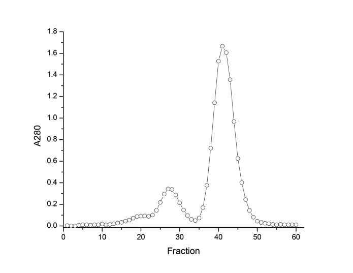
      4. Read the A_280/320 of peak fractions (Figure 1).

      5. Pool the central eight fractions from the major peak into a 50 ml conical tube.

      6. Measure the concentration spectrophotometrically, as described above.

      7. Dilute to 0.53 mg/ml by adding the PBS SEC buffer.

      8. Confirm the concentration spectrophotometrically.

      9. Add 0.5 ml aliquots to 1.5 ml bullet tubes, place in a freezer box, and place in a -80°C freezer.

2. Dynamic Light Scattering

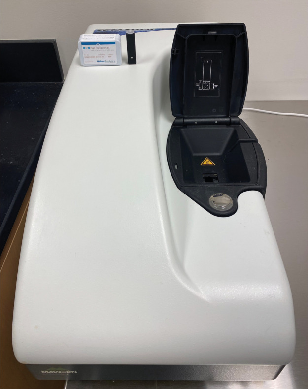
   The Zetasizer Nano S DLS instrument (Figure 2) uses a 632.8 nm He Ne red laser. It houses a single cuvette and measures light scattered at 173°. It is interfaced to a computer running Windows 10 and controlled with Zetasizer software. The scattering volume in the cuvette is automatically determined to allow for a large range of particle concentrations. Alternatively, the user can specify the position manually. A measurement consists of several averaged normalized intensity autocorrelation decays, called runs, each lasting 10 s. The number of measurements is specified by the user. The number of runs can either be determined automatically by the software based on the intensity of scattered light, which depends on the concentration and size of the macromolecule, or entered manually by the user. For BSA at 0.53 mg/ml, the number of runs is typically around 15. The runs are averaged in a manner that is not well described in the instrument documentation to produce a single z-average particle radius and polydispersity index. Additionally, the software produces an intensity particle diameter that is calculated using a user-specified algorithm that inverts the Fredholm integral (Eq. 14).

   In this protocol, a frozen BSA sample is thawed and prepared for analysis by ultrafiltration and high-speed centrifugation to remove possible large interfering scattering particles, as described below. A trial of four measurements is made on an aliquot. This process was repeated with fresh aliquots from the same thawed bullet tube for a total of eight trials to assess the variation due to aliquoting. Additionally, another sample of BSA is thawed and also subjected to eight trials, each with four measurements to assess possible variation due to freezing, thawing, and sample preparation.

   1. Instrument start-up

      1. Turn on the computer.

      2. Turn on the Zetasizer Nano S by pressing the power switch on the back of the instrument.

      3. The status light on the Zetasizer Nano S will initially be red.

      4. Start the Zetasizer Nano S software.

      5. The status light on the Zetasizer Nano S will become green.

      6. Select Tools > Count Rate Meter, select a temperature of 20°C, and enter Set.

      7. Place a ZEN2112 cuvette (Figure 2) in the instrument for temperature equilibration.

      8. Wait at least 30 min for the instrument to stabilize and the temperature to equilibrate.

   2. Preparation of a standard operating procedure (SOP)

      Measurements in the Zetasizer Nano S are made according to an SOP that is created by the user. The SOP specifies 1) the temperature and solvent viscosity, on which the diffusion rate depends and which are required for the calculation of hydrodynamic radius (Eq. 4), 2) the solvent refractive index, which is required for the calculation of the scattering vector (Eq. 11), 3) the number of measurements, and 4) the algorithm used in the calculation of the intensity distribution (Eq. 14). The viscosity for most common buffers can be estimated using SEDNTERP. Alternatively, it can be measured using a viscometer. The latter is preferable because errors due to the preparation of the buffer are not identified by SEDNTERP. The refractive index of buffers near physiologic ionic strength is only slightly increased from water, which is 1.333 at 632.8 nm laser wavelength and 20°C. For PBS used in this protocol, a value of 1.334 is used.

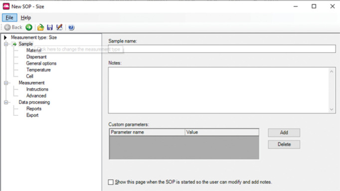
      1. Select File > New > SOP. A New SOP window appears (Figure 3):

         1. Measurement type: Select Size

         2. Material: Select Protein. (This selection is irrelevant for particles with a hydrodynamic radius less than 5% of incident wavelength, as is the case for BSA. However, there is no harm in selecting the Protein option.)

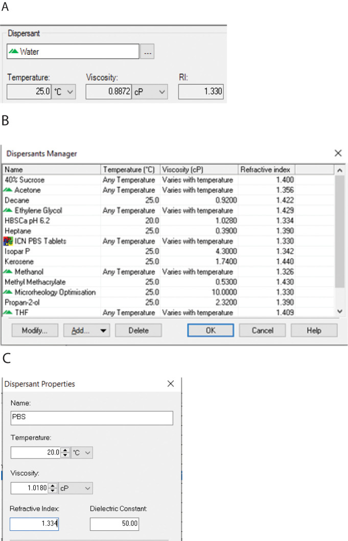
         3. Dispersant: The dispersant is the solvent. A window appears with the default, solvent water, or the last used dispersant (Figure 4A).

            1. Click the “…” (three dots) icon, and the Dispersants Manager window appears (Figure 4B).

            2. Select an existing solvent. A window will appear with the temperature, viscosity, and refractive index.

            3. Alternatively, add a new solvent by selecting Add… > Simple dispersant or solvent. A Dispersant Properties window will appear (Figure 4C). Enter a name for the solvent, the temperature, solvent viscosity, and refractive index. The dielectric constant is irrelevant, but a number must be entered. Enter 50. The new solvent will appear in the Dispersants Manager window.

         4. General Options: Select Use dispersant viscosity as sample viscosity. (The Mark-Houwink parameters are irrelevant for this analysis.)

         5. Temperature.

            1. The temperature is set by selecting the dispersant (see above).

            2. Equilibration time: Enter 30 s, which is sufficient for samples sitting at room temperature close to the measurement temperature of 20°C.

         6. Cell > Cell type > Quartz cuvettes Select ZEN2112.

         7. Measurement

            1. Measurement angle: Select 173° Backscatter

            2. Measurement duration: Select Automatic

            3. Number of measurements: Enter 4

            4. Delay between measurements: Enter 0 s

            5. Append measurement number to sample name: Check the box

            6. Artial results: Do not check the box

            7. Measurement duration > Extend duration for large particles. Enter No

            8. Positioning method: Select Seek for optimum position

            9. Automatic attenuation selection: Enter Yes

         8. Data Processing > Analysis model Select Protein Analysis

            Configure: Select Display range 0.1 to 6,000, upper and lower thresholds 0.01 and 0.05 (these are the default values).

      2. Save the SOP using File > Save as.

         NOTE: Be sure to add the extension *.sop, the program will not do it automatically.

      3. Place the SOPs in the folder \Malvern Instruments\Zetasizer\SOP\Protein. This folder is the default folder the program looks for to find an SOP file.

      4. Before every experiment, check the SOP for the correct settings by selecting File > Open > SOP > Protein and choosing the SOP.

   3. Preparation of a sample for measurement

      1. Remove a 0.5 ml aliquot of purified BSA from the -80°C freezer and thaw 15 min in a 37°C water bath.

      2. Remove the plunger of a Henke Sass Wolf 1 ml Tuberkulin syringe.

      3. Place a 0.02 μm Whatman Anotop10 filter on the syringe.

      4. Add the BSA to the barrel and filter into a 1.5 ml bullet tube.

      5. Centrifuge at 18,000 × g for 20 min at room temperature.

      6. Remove the top 0.45 ml and pipet into a fresh 1.5 ml bullet tube.

      7. Remove the cuvette from the Zetasizer Nano S instrument.

      8. Add 20 μl of sample by placing the pipet tip at the bottom of the cell. Do not fully expel the contents to avoid air bubbles. This volume leaves the meniscus in the viewing window of the cuvette, which is satisfactory. It is acceptable if the meniscus is uneven.

      9. Cap the cuvette and place in the Zetasizer Nano S instrument.

      10. After the measurements (see below), remove and dispel the old sample, repeating the extraction once. If repeating a trial with the same material, simply add 20 μl of fresh sample. If adding a solution containing a different macromolecule or concentration, wash the cell three times with 20 μl of the new solution, extracting the washes as described above, and then add 20 μl for measurement.

   4. Making DLS measurements

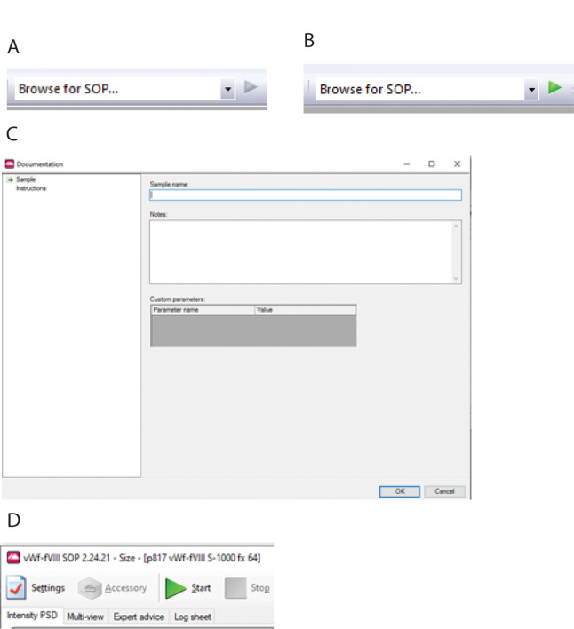
      1. When the Zetasizer software is started, a window appears entitled “Example results,” which lists several records. Close the window by selecting File > Close. Initially, the arrow next to Browse for SOP… on the Toolbar is greyed out (Figure 5A).

      2. Select File > New > Measurement file and give the file a name. A .dts file will be created.

      3. Save the file in the folder \Malvern Instruments\Zetasizer\Measurement Data. The small arrow next to Browse for SOP… becomes green (Figure 5B).

      4. Click on the small green arrow. A window appears for the selection of the SOP.

      5. Navigate to \Malvern Instruments\Zetasizer\SOP\Protein and select the appropriate SOP file. A Documentation window appears (Figure 5C). Enter a name for the sample. If a window appears that does not have OK at the bottom, selecting the SOP has been done incorrectly. Repeat the steps above.

      6. After selecting OK, a window appears with a big green arrow (Figure 5D). Click it to start the set of measurements. Initially, when the arrow is clicked, the measurements start after the user-specified equilibration period. On repeat trials, a message appears directing the user to insert the cell. After inserting the cell, click the big green arrow again, and the measurements will start.

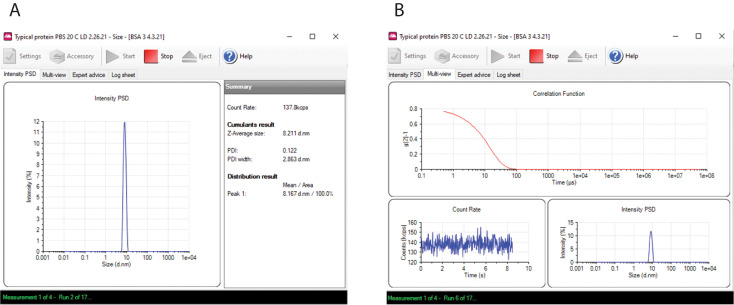
      7. As a series of runs accumulates into a measurement, select Intensity PSD, and a graph appears showing the distribution analysis as Intensity versus Size and cumulant analysis, showing the Z-average diameter and polydispersity index Figure 6A. At the completion of the run, the distribution function is calculated, and Intensity vs. Size is plotted. Then another run is executed, with continual updating of the intensity vs. size graph until the runs have been completed, which constitutes a single measurement.

      8. Alternatively, during measurements, select Multi-View, and a window appears showing: 1) g₂(τ) –1 versus decay time τ, which is updated as a run evolves; 2) the intensity fluctuations described in Background; and 3) the intensity distribution (Figure 6B). The intensity distribution for a monodisperse protein preparation should be monomodal and symmetric, as shown in Figures 6A and 6B. An example of polydisperse sample is shown in Figure 7, which was prepared by mixing BSA with thyroglobulin. If the intensity distribution is multimodal, the sample preparation should be repeated.

      9. After the measurements are complete, the measurement window displays the message Insert cell and press start when ready. Close it by clicking the X in the upper right corner.

      10. Close the window showing the records view by entering File > Close or clicking the red X on the upper right part of the window.

      11. Start another trial using the same SOP. Select File > New > Measurement file and enter a new file name. The existing SOP should still be present. Click the small green arrow. (NOTE: If the small green arrow is not present, the measurement window probably has not been closed.) When the SOP window appears, change the name of the sample and select OK as described above. The big green arrow should appear to start the next trial.

   5. Shutdown

      1. Exit Zetasizer software (File > Exit).

      2. Turn off the Zetasizer.

      3. Shut down computer.

   6. Cleaning the Zen2115 cuvette

      Wear powder-free gloves. Use a 200 μl pipette and 200 μl volumes.

      1. Withdraw the cuvette contents.

      2. Wash 5× with H₂O.

      3. Wash 5× with 2% (v/v) Hellmanex III.

      4. Wash 5× with H₂O.

      5. Wash 5× with H₂O:HCl:EtOH 2:1:1 (v:v:v).

      6. Wash 3× with H₂O.

      7. Wash 1× with 200 proof EtOH.

      8. Dry the cuvette in a vacuum desiccator.

Figure 1. Superdex 200 SEC of BSA.

Figure 2. Zetasizer Nano S particle size analyzer.

The ZEN2112 cuvette is shown next to the open sample compartment.

Figure 3. Zetasizer SOP window.

Figure 4. Dispersant properties.

(A) Default Dispersant window. (B) Dispersants Manager window. (C) Dispersant Properties window.

Figure 5. Making DLS measurements.

(A) initial Browse for SOP window. (B) Browse for the SOP window after a new measurement file has been created. (C) Documentation window. (D) Big green start arrow.

Figure 6. Measurement windows.

(A) Intensity PSD. (B) Multi-view.

Figure 7. Sample polydispersity.

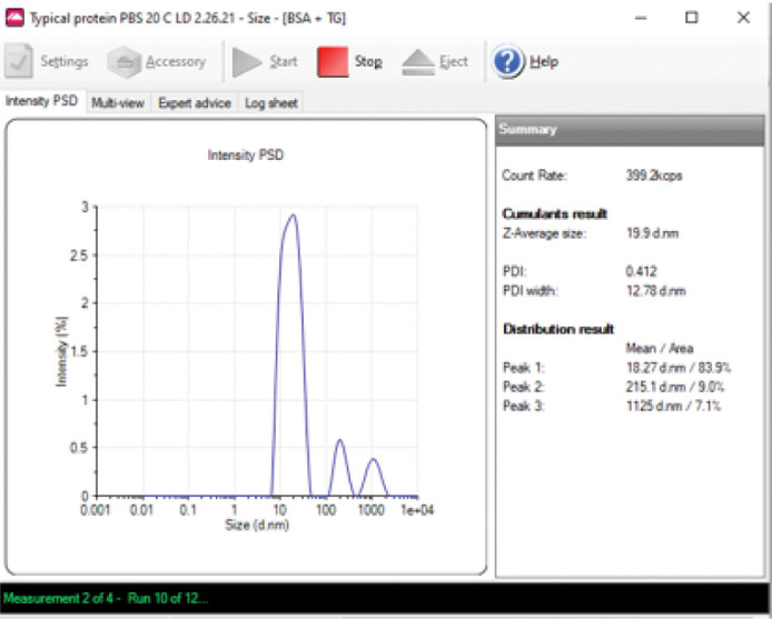
BSA and crude, unfiltered thyroglobulin were mixed at concentrations of 0.25 and 0.13 mg/ml, respectively.

Data analysis

1. Zetasizer analysis

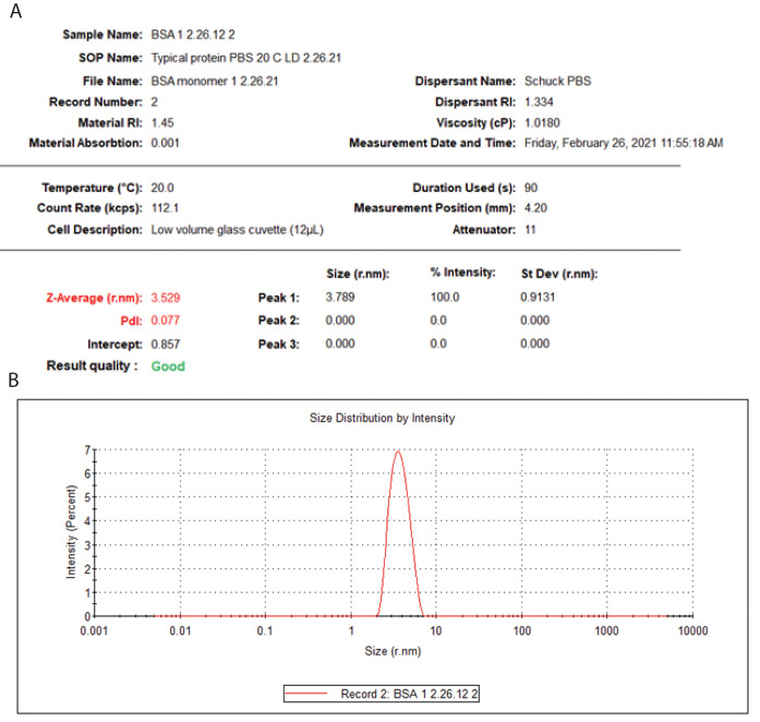
   1. At the completion of a set of measurements, select the Records View tab. Each Record corresponds to a single measurement. It lists the Z-average hydrodynamic radius, R_h, (or diameter if the user prefers) and polydispersity index (PdI) obtained by cumulant analysis and the hydrodynamic radii (or diameters) associated with peaks identified using distribution analysis (Figure 8). The results can be viewed either from individual measurements or collectively by selecting all measurements with the mouse.

   2. Ensure that the correct solvent was used by right-clicking on a measurement file and selecting Edit Result. A window will appear with solvent (dispersant) properties. If the wrong solvent has been used, make the correction by modifying the SOP.

   3. To view results as radius instead of diameter, click d.nm and change to r.nm.

   4. To get statistics, select all the records and means, and sample standard deviations for the set of measurements will appear.

   5. Select the Intensity PSD tab, which opens up a table that includes the count rate, measurement position in the cuvette, attenuation and size information, data relevant to the measurement (Figure 9A), and a graph of the particle size distribution (Figure 9B). The Volume PSD is not relevant to measuring the diffusion coefficient of proteins. The Size Quality Report evidently is primarily for commercial applications.

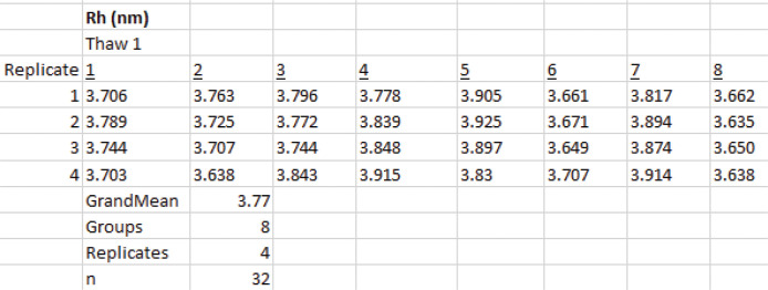
      1. Copy the z-average R_h and Pk1 Mean intensity R_h values (Figure 8) and paste into an Excel file for later use. There will be 32 values corresponding to four measurements on eight aliquots.

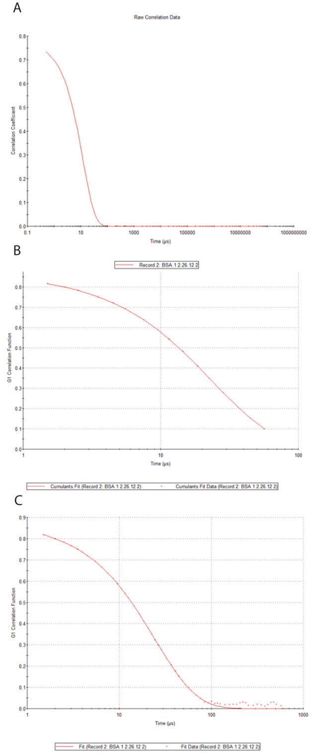
   6. Select Correlogram (M), which displays a graph of Correlation Coefficient versus Time (Figure 10A). “Correlation Coefficient” is the quantity g₂(τ) –1. Time is the decay time, τ.

   7. Select Cumulants Fit (M), and a graph appears showing G1 Correlation Function versus Time data fitted using cumulant analysis (Figure 10B). The G1 Correlation Function is the normalized field autocorrelation function, g₂(τ) . Note that data are only fitted for g1(τ) values greater than 0.1.

   8. Select Distribution Fit (M), and a graph appears showing G1 Correlation Function versus Time data fitted using distribution analysis (Figure 10C).

2. SEDFIT analysis

   1. Converting Zetasizer files to SEDFIT compatible files

      Zetasizer record files, which contain the results of a single measurement, have the suffix .dts. They can be converted to files that SEDFIT can read using a macro in Zetasizer software under Tools > Macros > Make DLSDAT-v1-0.

      1. Create the .dlsdat macro

         1. Go to www.materials-talks.com/blog/2015/10/28/new-macro-to-export-dls-data-to-sedfit/. Select Method 1.

         2. Download and unzip MakeDLSDAT-v1-0.zip by clicking on the link at the above site. MakeDLSDAT-v1-0.zmac appears in the /Downloads folder. Move it to the Desktop.

         3. Start the Zetasizer software.

         4. Go to Tools > Options > Macros > Install new Macro.

         5. Select MakeDLSDAT-v1-0.zmac from the Desktop.

         6. Restart the Zetasizer software. Now under Tools > Macros, Make DLSDAT-v1-0 appears.

      2. Using the dls.dat macro

         1. In the Zetasizer software, select File > Open > Measurement File and navigate to the folder containing the desired .dts file. A .dts file contains a set of measurements, which appear as separate records. Each measurement can be converted to a .dlsdat file.

         2. Open a .dts file by selecting Open > Measurement file and highlight a record under Records View. Right-click Macros > MakeDLSDAT-v1-0 and enter a file name. The macro will produce a file with the extension .dlsdat for use with SEDFIT.

      3. Properties of .dlsdat files

         Each .dlsdat file contains a header and about 200 data pairs. Figure 11 shows an example of the header and the first few lines of a .dlsdat file.

         In the header, 19.998910 is the temperature, 1.334 is the solvent refractive index, 0.010018 is the solvent viscosity in Poise, 173 is the scattering angle, and 6.328e-07 is the wavelength of the helium-neon laser in meters. SEDFIT calculates the scattering vector according to Eq 11. The first column of data is the delay time, $\tau$, in seconds. The second column is g₂(τ) –1.

   2. SEDFIT cumulant analysis

      1. Run SEDFIT, select Data > Load DLS data and load a .dlsdat file. SEDFIT takes the square root of g₂(τ) –1 in the .dlsdata file to produce g1(τ) (which it calls g(1) field autocorrelation). The SEDFIT default is to graph and fit g1(τ) data. Instead, graph and fit g₂(τ) –1 data by selecting Options > DLS Tools > Toggle Intensity <-> Field Autocorrelation Fct, which toggles the SEDFIT graph between “intensity autocorrelation function” and “field autocorrelation function”.

      2. Select Options > DLS Tools > Always Load Intensity Autocorrelation g(2)–1.

      3. Use the mouse to move the green vertical lines to set the fitting limits. Select the left fitting limit to include the first data point. Select a right fitting limit of about 1 log to the right of where the data has approached zero (Figure 12). Selecting more data does not improve the fitted constants.

      4. Select Model > Dynamic Light Scattering > Cumulant Analysis.

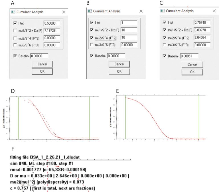
      5. Select Parameters, and the default Cumulant Analysis window appears (Figure 13A). “I tot” refers to the value of g₂(τ) –1 at zero τ. mu1/S^2 = Dz is $\stackrel{-}{\mathrm{\Gamma }}$ (Eq. 15). mu2 and mu3 are the moments μ₂ and μ₃ (Eq. 15). S is the magnitude of the scattering vector (q in Eq. 11). The units of the parameters are F, F^2, and F^3, respectively, where 1 F is 1 Fick and is equal to 1 cm² s^-1.

      6. Fit I tot, Dz and mu2/S^4 and Baseline by checking the boxes and entering initial guesses. mu3/S^4 is not fitted. Enter a starting value for Dz above the anticipated value. The same value can be entered for mu2/S^4. Enter a value 1 of I tot and a value of zero for Baseline. In practice, the fitting is very robust with respect to initial estimates and reproducibly converges to the same values. The initial estimates are shown in Figure 13B.

      7. Select Run. SEDFIT calculates g₂(τ) –1 using the initial estimates and Eq. 15(Figure 13D). In this example, the initial fit follows the data to some extent but requires optimization, which is done by nonlinear least-squares analysis using the Marquardt Levenberg algorithm.

      8. Select Options > Fitting Options > Marquardt Levenberg.

      9. Select Fit. Now optimization of the parameters produces a close fit to the data (Figure 13E). (Select Display > Update to display only the graph).

      10. Select Parameters to see the fitted constants (Figure 13C). In this example, D_z is 6.03 F.

      11. Enter Display > Show Last Fit Info Again or type “Ctrl o,” and the fitting information will be superimposed on the graph, including the root mean squared deviation (rmsd) of the fit and the polydispersity index (Figure 13F). In this example, the polydispersity is 0.073.

      12. Some of the information displayed (not shown in the figure) is in reference to fitting sedimentation data and is irrelevant.

      13. Record the D_z values in an Excel spreadsheet for later use. There will be 32 values corresponding to four measurements on eight aliquots.

   3. SEDFIT continuous I(D) distribution analysis

      1. In SEDFIT, load DLS data as described above under Data analysis B.2 and select Model > Dynamic Light Scattering > DLS:Continuous I(D)-Distribution.

      2. In contrast to cumulant analysis, in which fitting is done to g₂(τ) –1 values, fitting must be done to g1(τ) in this model. Select Options > DLS Tools > Toggle Intensity <-> Field Autocorrelation Fct and toggle to “field autocorrelation function”. The graph displays a plot of g1(τ) versus τ (not shown).

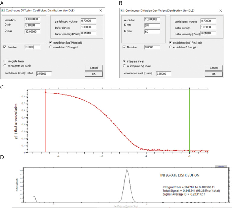
      3. Select Parameters. The Parameters window appears (Figure 14A).

      4. There are several possible combinations of starting parameter estimates. Select the default values equidistant log(1/tau) grid, integrate linear, and resolution equal to 100. Leave the confidence level (F-ratio) at the default value of 0.55 as recommended at www.analyticalultracentrifugation.com. The partial specific volume, buffer density, and buffer viscosity are irrelevant. Make initial starting estimates of D min and D max that are 10-fold below and above the estimated value of the diffusion coefficient. For BSA, values of 0.6 and 60 are selected (Figure 14B).

      5. Select Run. An apparent idiosyncrasy of the program is that, in contrast to cumulant analysis, the Run command does a nonlinear least-squares fit. An upper window appears, showing the fit (Figure 14C). The lower window shows the fitted distribution (Figure 14D). As in the Zetasizer software, the presence of aggregates or impurities can produce several peaks indicative of polydispersity (not shown).

      6. Calculate the signal-average diffusion coefficient by clicking the integrate button (Figure 14D, upper right corner) and selecting the region containing the distribution using the right mouse button as directed in the program. In this example, a signal average diffusion coefficient of 6.203 F was obtained (Figure 14D, inset).

      7. Record the signal average diffusion coefficient values in an Excel spreadsheet for later use.

3. Excel Solver analysis

   In this example, the Excel GRG unweighted nonlinear least-squares regression algorithm is used to fit the results from a single Zetasizer measurement of the BSA DLS decay to the first two moments of the Frisken cumulant equation (Eq. 15)

   $$g_2\left(\tau \right)=B+ \beta exp\left(-2\stackrel{-}{\mathrm{\Gamma }}\tau \right){\left(1+\frac{{\mu }_2}{2!}{\tau }^2\right)}^2$$

   This protocol assumes familiarity with Excel and that the Solver add-in has been installed.

   1. Run Excel and name a blank sheet “Master Sheet.”

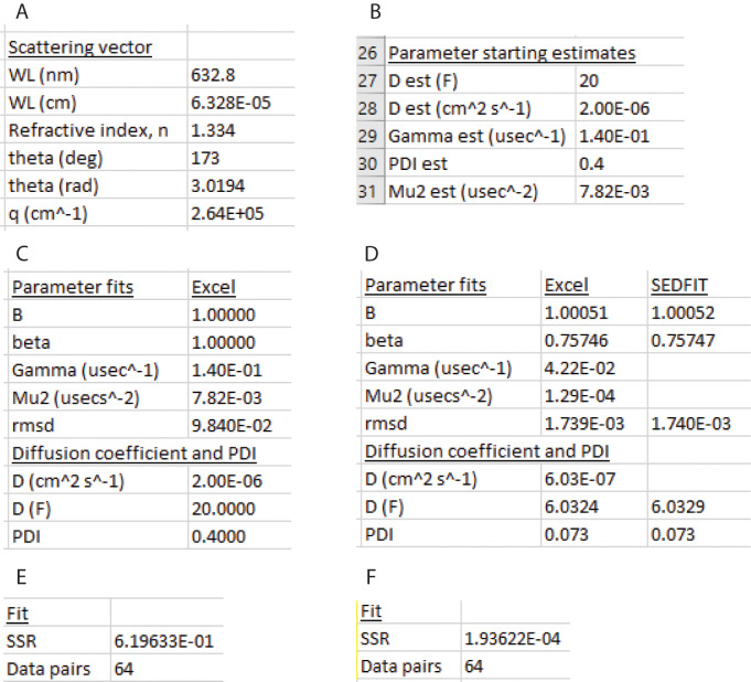
   2. Create a table to calculate the magnitude of the scattering vector in cells I26:J32 (Figure 15A).

   3. In column I, enter row labels (“WL (nm),” “WL (cm),” etc.).

   4. In column J, enter the values for the DLS laser wavelength, solvent refractive index, and scattering angle in degrees. Convert the scattering angle to radians. Use the Excel function Define Name and define the names WL, RI, and theta_rad. Calculate the magnitude of the scattering vector, q (Eq. 11):

      $$q=\frac{4\pi n}{\lambda } sin\left(\frac{\theta }{2}\right)$$

      The Excel code for this equation using the defined names is “4*PI()*RI*SIN(theta_rad/2)/W.”

   5. Create a set of column names tau (s), tau (usec), g2-1, g2, and g2 calc in columns A, B, C, D, and E in row 37 (Figure 16).

   6. Import a .dlsdat file containing g₂(τ) –1 vs. τ data by selecting Data > From Text/CSV, then Load. Data will load as a single column in a new sheet.

   7. Select the column of loaded data, then select Data > Text to Columns, Delimited, Space. Columns of τ and g₂(τ) –1 will be created. Delete the three header rows.

   8. Cut and paste τ and g₂(τ) –1 data into columns A and C of the Master Sheet, respectively, starting at row 38 (Figure 16). Use the same number of data pairs as in the SEDFIT cumulant fit.

   9. Convert τ from seconds to microseconds (to avoid a numerical precision problem) by multiplying the values in column A by 1E6 and place the values in col B (Figure 16).

   10. Calculate g₂(τ) by adding 1 to the values in column C and place the values in column D (Figure 16).

   11. Make a table of Parameter starting estimates starting in row 26 (Figure 15C). Enter a starting estimate of the diffusion coefficient in Ficks in row 26. In this example, a starting estimate of 20 F has been entered. Convert to units of cm² s^-1 by multiplying by 1E-07. Calculate an estimated value of $\stackrel{-}{\mathrm{\Gamma }}$, and label it Gamma est using the first moment form of Eq. 10:

       $$\stackrel{-}{\mathrm{\Gamma }}=D_z{q}^2$$

   12. Enter a starting estimate for the polydispersity index (PDI). In this example, a starting value of 0.4 has been entered. Calculate an estimated value of the second moment, μ₂, and label it Mu2 est using Eq. 17:

       $${\mu }_2=\left(PDI\right){\stackrel{-}{\mathrm{\Gamma }}}^2$$

   13. Make a table Parameter fits starting in row 26 and a table Diffusion coefficient and PDI starting in row 32 (Figure 15D).

   14. Copy the values of Gamma_est and Mu2_est into the Parameter fits table. Enter 1 for starting estimates for both B and β. Define names for the values in the Parameter Fits table: B_, beta, Gamma, Mu_2. Figure 15C shows the Parameter Fits table before Solver has run.

   15. Calculate g₂(τ) from the starting estimates using the first two moments of the Frisken equation (Eq. 15). The Excel code for this calculation is:

       B_+beta*EXP(-2*Gamma*B38)*(1+(Mu_2*B38^2/2))^2

       where B38 represents the value of τ in the first row of data.

   16. Make a table entitled Fit starting in row 26 with rows SSR and Data pairs. Figure 15E shows the values of SSR before Solver has run.

   17. Calculate the summed squared residuals (SSR) from the g2 and g2 calc columns using the SUMXMY2 function in Excel. In this example, the g2 and g2 calc values are in rows D38:D101 and E38:E101, respectively (Figure 16), and the Excel code is:

       SUMXMY2(D38:D101,E38:E101)

       Determine the number of data pairs using the Excel COUNT function or by entering it manually.

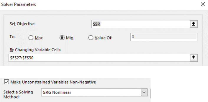
   18. Minimize SSR by fitting the parameters B, beta, Gamma, and Mu2 that are in cells E27:E30 using the GRG Nonlinear algorithm in Solver by selecting Data > Solver, Set Objective SSR, To Min, By Changing Variable Cells $E$27:$E$30 (Figure 17). In this example, the SSR has decreased from 1.94E-04 after Solver has run (Figure 15F). The fitted parameters and estimates of the diffusion coefficient and PDI appear in the Parameter fits and Diffusion coefficient and PDI tables (Figure 15D). The rmsd has decreased from 0.098 to 1.74E-03 (Figure 15D).

   19. Cut and paste SEDFIT cumulant estimates of B, beta (called “I tot” in SEDFIT), rmsd, D, and PDI for comparison (for B, add 1 to the SEDFIT fitted baseline). The values are in close agreement (Figure 15D).

4. Statistical analysis

   1. Point estimates and confidence intervals by analysis of variance

      The goal of this protocol is to assign a point estimate and a 95% confidence interval for the diffusion coefficient of BSA, corrected to the standard condition of water at 20°C, D_20,w. A trial of four measurements (replicates) is made on a sample. The process was repeated with fresh aliquots from the same tube for a total of eight trials. Additionally, another sample of BSA is thawed and also subjected to eight trials, each with four measurements, to assess possible variation due to freezing and thawing.

      Possible sources of variation in the experimental results arise from: 1) the variation within a trial of four measurements; 2) variation between trials due to removing the cuvette and repeated aliquoting; and 3) variation due to freezing, thawing, and sample preparation. The variation due to replication and repeated aliquoting is assessed by one-way random effects analysis of variance (ANOVA), which produces a point estimate and 95% confidence interval for the diffusion coefficient. Although there are many sources that describe one-way random effects ANOVA, few provide derivations of the confidence interval. One example is Brownlee (1965), which provides the basis for the description that follows.

      In one-way ANOVA, there are a independent groups of samples (here, aliquots), each of which has b measurements (replicates). The ANOVA model is

      $$X_{j,k}=\mu +{\alpha }_j+{\epsilon }_{j,k}$$

      where X_j,k is the measurement associated with the replicate k of group j, μ is the grand mean of the measurements of all the groups, α_j is the mean of group j, and ε_j,k is the error associated with measurement within the group j, measurement k. It is assumed that α_j are normally distributed with zero mean and variance ${\sigma }_B^2$ and that ε_j,k is normally distributed with zero mean and variance, ${\sigma }_W^2$. The variance of X is given by

      $${\sigma }_X^2={\sigma }_B^2+{\sigma }_W^2$$

      The terms on the right are called the components of variance. In this example, we are interested in the mean, μ(the point estimate) and confidence limits of the diffusion coefficient of BSA.

      The hypothesis tested in the random effects model is

      $$H_0: {\sigma }_B^2=0$$

      i.e., all variation is due to replication, and there is no variation because of group effects. It is equivalent to the hypothesis

      $$H_0: {\alpha }_j=0$$

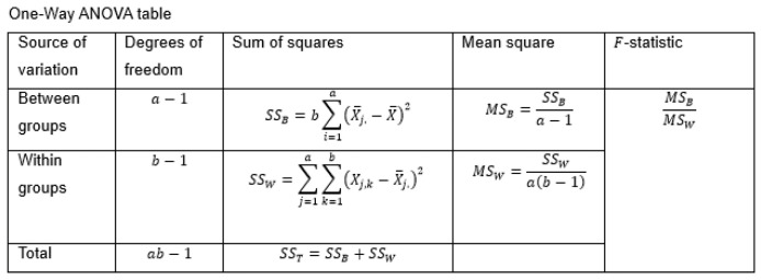
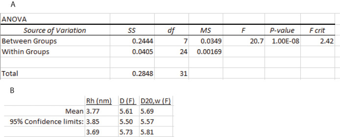
      Results are summarized using an ANOVA table (Figure 18):

      In the table, $\stackrel{-}{X}$, is the sample grand mean and ${\stackrel{-}{X}}_{j.}$ is the mean of the replicates of group $j$. The hypotheses, H₀, is tested using F statistics where

      

      with a–1, b–1 degrees of freedom. The estimator of the variance within groups is

      

      The estimator of ${\sigma }_B^2$ is

      

      The estimator of the variance of the mean, $\stackrel{-}{X}$, is

      

      Equivalently,

      

      The 95% confidence interval for μ is obtained from Student’s t-distribution with a–1 degrees of freedom.

      

      where $\stackrel{-}{X}$ is mean of all measurements, –t_0.975 and t_0.975 are the values of t-distribution for which 2.5% of the area lies within each tail of the distribution, and ${\widehat{\sigma }}_{\stackrel{-}{X}}$ is the estimator of the standard deviation of the mean (also called the standard error of the mean). One-way ANOVA can be performed using Excel. This example assumes the Data Analysis Add-In has been installed.

   2. SEDFIT cumulant analysis statistics

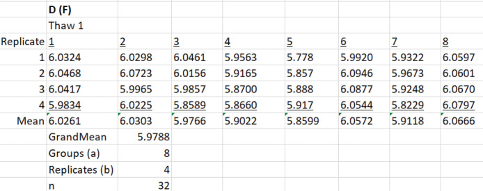
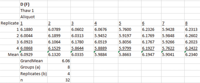
      1. Create a new worksheet in Excel and make eight columns for the aliquots and four rows for the measurements (replicates) (Figure 19).

      2. Select all 32 measurement values from Data analysis B.2 and calculate the sample grand mean using the Excel AVERAGE function. This is the estimate of D_z.

      3. Use the Define Name function to assign names to the number of groups and replicates in Figure 19.

      4. Select Data > Data Analysis > Anova: Single factor.

      5. In the window that appears, select the cells that contain the D values, $B$17:$I$20$ (Figure 20). The trials (aliquots) are grouped by columns.

      6. Select Alpha of 0.05. This is the significance level for the F test.

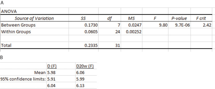
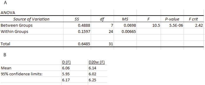
      7. Select $L$21 for the cell where the output range begins and then select OK. Excel produces an ANOVA table (Figure 21A). The F test reveals what is evident from the inspection of Figure 19, namely, that there is more variation between trials than between the measurements (replicates). Because the aliquots are taken from the same bullet tube, the variation is not due to pipetting error. Possibilities include small bubbles in the sample, reflection off the meniscus, or variation in the position of the cuvette during the process of removing it, adding a new aliquot, and replacing it.

      8. Calculate the confidence interval

         1. Calculate the variance of the mean by dividing the mean square between groups MS_B (Figure 21) by n, the total number of measurements.

         2. Calculate the standard deviation of the mean by taking the square root of this value.

         3. Calculate the value of Student’s t density function for a 95% confidence interval using the Excel function T.INV(probability,deg_freedom). Here, the probability is 0.975, and the degree of freedom is a–1. Since a equals 8, there are 7 degrees of freedom and T.INV(0.975, 7) = 2.365.

         4. Calculate the upper and lower limits of the confidence interval using Eq. 24.

         5. Calculate D_20,w using Eq. 5:

            $$D_{20,w}=D\frac{T_{20}}{T}\frac{\eta }{{\eta }_{20,w}}$$

      The point z-average estimates of D and D_20,w are shown in Figure 21B.

   3. SEDFIT continuous I(D) distribution analysis statistics

      1. Create a new worksheet in Excel and make eight columns for the aliquots and four rows for the measurements as Data analysis D.2 (Figure 22).

      2. Insert the measurement values from the SEDFIT continuous I(D) distribution analysis from Data analysis B.3 and calculate the grand mean. This is the signal-average diffusion coefficient.

      3. Construct an ANOVA table and calculate the calculate confidence limits as described in Data analysis D.2 (Figure 23).

   4. Zetasizer cumulant analysis statistics

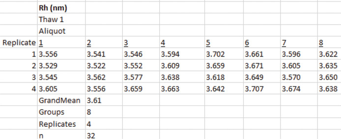
      1. Create a new worksheet in Excel and make eight columns for the aliquots and four rows for the measurements (replicates) as in Data analysis D.2 (Figure 24).

      2. Insert the measurement values of R_h from the Zetasizer cumulant analysis Data analysis A and calculate the grand mean.

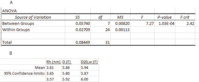
      3. Construct an ANOVA table and calculate the confidence limits for R_h as described Data analysis D.2. Convert R_h values to z-average diffusion coefficients, D and D_20,w, using the Stokes-Einstein equation (Eq. 4). The results are shown in Figure 25.

   5. Zetasizer “Protein Analysis” distribution statistics

      1. Create a new worksheet in Excel and make eight columns for the aliquots and four rows for the measurements as in Data analysis D.2 (Figure 26).

      2. Insert the measurement values of R_h from Zetasizer Protein Analysis Data analysis A and calculate the grand mean.

      3. Construct an ANOVA table and calculate the confidence limits for R_h as described in Data analysis D.2.Convert R_h values to signal-average diffusion coefficients, D and D_20,w, using the Stokes-Einstein equation (Eq. 4). The results are shown in Figure 27.

   6. Testing possible variation due to freeze-thawing followed by sample preparation

      1. Thaw a new sample and repeat the sample preparation steps described in Procedure B.3

      2. Perform DLS measurements and analysis on eight aliquots of the sample, four measurements per aliquot as described in Procedure B.4 and Data analysis.

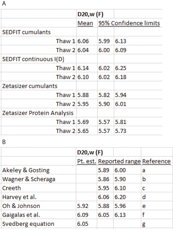
      3. Compare the results to the first thawed sample (Figure 28A). The results show overlapping confidence intervals for all four methods of analysis, indicating there is no systematic error due to the freeze-thaw sample preparation process.

   7. Summary of fitting methods and literature review

      The confidence intervals in Figure 28A are a measure of the precision but not the accuracy of the measurements and analysis. The goal of the protocol is to have a method of measurement and analysis that is free from significant systematic errors and produces a confidence interval that closely brackets a true value of the diffusion coefficient at infinite dilution at 20°C in water ($D_{20,w}^0$). It is important to address what is meant by $D_{20,w}^0$. Although diffusion coefficients are not measured at infinite dilution, the values for globular proteins typically show negligible variation at submilligram per mL concentrations, as is the case in this protocol. This specifically has been shown for BSA (Creeth, 1952). As noted in Background, the notion of a single diffusion coefficient is restricted to a two-component system, namely the macromolecule and solvent water. Because proteins are polyelectrolytes and carry net charge that varies with pH, it would seem fanciful to attempt to extrapolate from a buffered salt solution to water. However, the screening effects in solutions close to physiologic anionic strength tend to eliminate solvent-specific effects on diffusion, which again is the case with BSA (Creeth, 1952).

      Assuming it is realistic to think of a true $D_{20,w}^0$, the fundamental problem arises that it is never possible to know that all sources of systematic error have been eliminated. Consequently, measurement accuracy often is defined in terms of a reference value (Mandel, 1964). For example, the speed of light in vacuo is not known exactly from experiment but rather is defined as 299,792,458 m/s. Other measurements are made relative to this standard. In the absence of a reference standard, as with $D_{20,w}^0$ values, the evaluation of accuracy becomes an educated guess (Mandel, 1964). There are two ways to attempt to make a reasonable estimate. The first is to attempt to identify and estimate the size of all possible systemic errors and produce a range within which the true value is thought to lie. The second is to compare the results of independent measuring processes. For the $D_{20,w}^0$ value of BSA, three independent methods are diffusiometry, DLS, and application of the Svedberg equation. In diffusiometry, the measurements by Creeth reported in 1958 (Creeth, 1958) represented an evolution of improvements in the method and can be considered the most accurate measurements that are available (Figure 28B).

      The Svedberg equation (Eq. 18) can be rearranged to yield the diffusion coefficient as a function of the sedimentation coefficient, gas constant, temperature, molar mass, partial specific volume, and solvent density:

      $$D=\frac{sRT }{M\left(1-\stackrel{-}{\nu }\rho \right)}$$

      Of these, the experimental determination of the sedimentation coefficient extrapolated to water at 20°C, $s_{20,w}^0$, and the uncertainty the partial specific volume, $\stackrel{-}{\nu }$, are the most significant sources of error. Without doing a formal propagation of errors analysis, using a measured value of $s_{20,w}^0$ of 4.44 S (Parker and Lollar, 2021), $\stackrel{-}{\nu }$ = 0.733 ml/g using the BSA amino acid composition and the partial specific volume calculator in SEDFIT, M = 66,365 g/mol, and ρ_20,w = 0.9982 g/ml, yields a diffusion coefficient of 6.05 F (Figure 28B), which is within the Creeth’s diffusiometry confidence interval.

      Of the data analysis methods in this protocol, the continuous I(D) method and Protein Analysis method yield confidence intervals that are less precise than the cumulant methods. The SEDFIT cumulant confidence intervals cover the estimates from diffusiometry and the Svedberg equation better than the Zetasizer cumulant analysis, which produces lower values. The SEDFIT cumulant analysis also is preferable because the equation it is fitting is Frisken equation, as verified independently using Excel Solver. Fitting data to the Frisken equation represents an improvement to earlier methods because it uses nonlinear least-squares regression instead of transforming the g₂(τ) logarithmically and performing a linear regression. In contrast, the Zetasizer cumulant method is not described on the software documentation. It truncates the data set at low values of g₂(τ) –1, possible due to a logarithmic transform that must avoid fitting values that vary around zero.

      Figure 28. ${\mathit{D}}_{20,\mathit{w}}^0$ of BSA.

      

      (A) Point estimates (Pt. est) and 95% confidence limits for the z-average $D_{20,w}^0$ this protocol. (B) Literature the $D_{20,w}^0$ values.

      a: Ref. (Akeley and Gosting, 1953), diffusion cell, Gouy interferometry, 0.01 M K acetate, 0.15 M KCl, pH 4.59, corrected for impurity

      b: Ref. (Wagner and Scheraga, 1956), diffusion cell, Gouy interferometry, 0.5 M KCl, pH 5.14; corrected for impurity

      c: Ref. (Creeth, 1958), diffusion cell, Rayleigh interferometry, 0.01 M K acetate, 0.15 M KCl, pH 4.59, corrected for impurity

      d: Ref. ( Harvey et al., 1979 ), DLS, cumulant analysis, SEC fractionated BSA; 0.1 M NaCl, 0.07 M phosphate, pH 7.0

      e: Ref. (Oh and Johnson, 1981), DLS, cumulant analysis, SEC fractionated BSA, 0.1 M NaCl, 0.02 M sodium acetate, pH 4.7

      f: Ref. ( Gaigalas et al., 1992 ), DLS, cumulant analysis, NIST standard BSA, various buffers

      g: Svedberg equation (Eq. 18, see text)

      The ranges reported refer to undefined confidence intervals or error estimates.

Figure 8. Records View.

Figure 9. BSA DLS measurement results.

(A) Tabulated results. (B) Particle size distribution.

Figure 10. DLS decays.

(A) g₂(τ) –1 vs. τ. (B) Zetasizer cumulants fit. (C) Zetasizer distribution fit.

Figure 11. Structure of a .dlsdat file.

Figure 12. SEDFIT fitting limits.

Figure 13. SEDFIT DLS cumulants fit.

(A) Opening parameter window. (B) Initial parameter estimates. (C) Fitted parameters. (D) Calculated g₂(τ) –1 values from initial estimates. (E) Fitted curve.

Figure 14. SEDFIT DLS continuous I(D) distribution fit.

(A) Default continuous I(D) window. (B) User-selected continuous I(D) values. (C) Fitted g1(τ) decay curve. (D) Fitted continuous I(D) distribution, which is integrated to produce the signal-average diffusion coefficient.

Figure 15. Excel Solver DLS cumulant fit.

(A) Scattering vector. (B) Parameter starting estimates. (C) Parameter fits before running Solver. (D) Parameter fits after running Solver with the SEDFIT fitted parameters shown for comparison. (E-F) SSR before and after running Solver.

Figure 16. DLS data and Excel Solver cumulant fits.

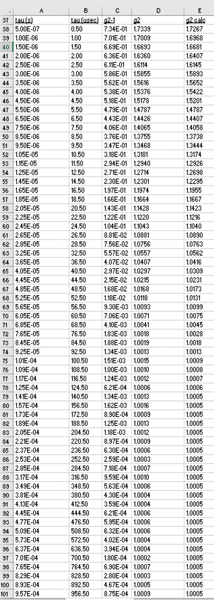
Column A, imported values of τ; column B, conversion of τ to μs; column C, imported values of g₂(τ) –1; column D, g₂(τ) ; column E, the fitted values of g₂(τ) .

Figure 17. Excel solver window.

Figure 18. ANOVA table.

Figure 19. SEDFIT cumulant fits.

Figure 20. Excel ANOVA window.

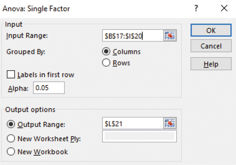
Figure 21. SEDFIT cumulants ANOVA.

(A) ANOVA table. (B) Point estimate and confidence limits for z-average D and z-average D_20w.

Figure 22. SEDFIT continuous I(D) fits.

Figure 23. SEDFIT continuous I(D) ANOVA.

(A) ANOVA table; (B) Point estimate and confidence limits for z-average D and z-average D_20w.

Figure 24. Zetasizer cumulants Rh fits.

Figure 25. Zetasizer cumulants ANOVA.

(A) ANOVA table. (B) Point estimate and confidence limits for z-average D and z-average D_20w.

Figure 26. Zetasizer Protein analysis Rh fits.

Figure 27. Zetasizer Protein Analysis ANOVA.

(A) ANOVA table. (B) Point estimate and confidence limits for z-average $D$ and z-average D_20w.

Recipes

1. 10× PBS (1 L)

   1.54 M NaCl

   56 mM Na₂HPO₄

   10.6 mM KH₂PO₄

   1. Weigh out:

      For 1.54 M NaCl (MW 58.44) 90. 0g

      For 56 mM Na₂HPO₄ (MW=141.96) 7.95 g

      For 10.6 mM KH₂PO₄ (MW 136.09) 1.44 g

   2. Add the solids to ~980 ml H₂O in a 1 L beaker

   3. After dissolution, adjust volume to 1 L in a graduated cylinder

   4. Filter using a Corning 500 ml, 0.22 μm filter apparatus

   5. Store at 4°C

2. PBS (1 L)

   0.154 M NaCl

   5.6 mM Na₂HPO₄

   1.06 mM KH₂PO₄, pH 7.4

   1. The densities of 10× PBS and water at 20°C calculated using SEDNTERP are 1.0684 g/ml and 0.9982 g/ml, respectively.

   2. Add 100 ml 10× PBS gravimetrically to a 1 L Pyrex bottle (mass = density × volume = 106.8 g).

   3. Dilute with 900 ml H₂O gravimetrically (mass = density × volume = 898.4 g).

   4. The pH should be ~7.15. pH to 7.40 with 5 N NaOH using a pH meter.

   5. Filter as described above.

   6. Store at 4°C.

Competing interests

We have no competing interests to declare.

Ethics

There are no human subjects or animal studies described in this protocol.

References

- 1. Akeley D. F. and Gosting L. J.(1953). Studies of the diffusion of mixed solutes with the Gouy diffusiometer. J Am Chem Soc 75(22): 5685-5696. [Google Scholar]
- 2. Annunziata O., Buzatu D. and Albright J. G.(2005). Protein diffusion coefficients determined by macroscopic-gradient Rayleigh interferometry and dynamic light scattering. Langmuir 21(26): 12085-12089. [DOI] [PubMed] [Google Scholar]
- 3. Berg H. C.(1983). Random Walks in Biology. Princeton, Princeton University Press.
- 4. Berne B. J. and Pecora R.(1976). Dynamic Light Scattering with Applications to Chemistry, Biology, and Physics. Mineola, Dover Publications.
- 5. Bhattacharjee S.(2016). DLS and zeta potential- What they are and what they are not? J Control Release 235: 337-351. [DOI] [PubMed] [Google Scholar]
- 6. Brautigam C. A.(2019). Applications and complementarity of analytical ultracentrifugation and light scattering. Chapter 11. In: Biomolecular and Bioanalytical Techniques: Theory, Methodology and Applications 255-278. [Google Scholar]
- 7. Brownlee K. A.(1965). Statistical Theory and Methodology in Science and Engineering. In: A Wiley Publication in Applied Statistics. New York, John Wiley& Sons. [Google Scholar]
- 8. Cantor C. R. and Schimmel P. R.(1980). Biophysical chemistry: Part II Techniques for the study of biological structure and function. Oxford, W. H. Freeman and Company 591-642.
- 9. Creeth J. M.(1952). The use of the Guoy diffusiometer with dilute protein solutions- an assessment of the accuracy of the method. Biochem J 51(1): 10-17. [DOI] [PMC free article] [PubMed] [Google Scholar]
- 10. Creeth J. M.(1958). Studies of free diffusion in liquids with the Rayleigh method. III. The analysis of known mixtures and some preliminary investigations with proteins. J Phys Chem 62(1): 66-74. [Google Scholar]
- 11. Einstein A.(1926). Investigations on the Theory of Brownian Movement.(English translation first). New York, Methuen Co.& Dover Publications. pp124.
- 12. Finsy R.(1994). Particle sizing by quasi-elastic light scattering. Adv Colloid Interface Sci 52: 79-143. [Google Scholar]
- 13. Frisken B. J.(2001). Revisiting the method of cumulants for the analysis of dynamic light-scattering data. Applied Optics 40(24): 4087-4091. [DOI] [PubMed] [Google Scholar]
- 14. Gaigalas A. K., Hubbard J. B., McCurley M. and Woo S.(1992). Diffusion of bovine serum albumin in aqueous solutions. J Phy Chem 96(5): 2355-2359. [Google Scholar]
- 15. Harvey J. D., Geddes R. and Wills P. R.(1979). Conformational studies of BSA using laser light scattering. Biopolymers 18(9): 2249-2260. [Google Scholar]
- 16. Hurton T., Wright A., Deubler G. and Bashir B.(2012). SEDNTERP. http://bitc.unh.edu.
- 17. Koppel D. E.(1972). Analysis of macromolecular polydispersity in intensity correlation spectroscopy- method of cumulants. J Chem Phys 57(11): 4814-4820. [Google Scholar]
- 18. Mandel J.(1964). The Statistical Analysis of Experimental Data. New York, John Wiley and Sons.
- 19. Miller D. G.(2014). The history of interferometry for measuring diffusion coefficients. J Solution Chem 43(1): 6-25. [Google Scholar]
- 20. Ogendal L. H.(2017). Light Scattering Demystified: Theory and Practice. Danmark, University of Copenhagen.
- 21. Oh Y. S. and Johnson C. S.(1981). The wave vector dependence of diffusion-coefficients in photon-correlation spectroscopy of protein solutions. J Chem Phys 74(5): 2717-2720. [Google Scholar]
- 22. Parker E. T. and Lollar P.(2021). Conformation of the von Willebrand factor/factor VIII complex in quasi-static flow. J Biol Chem 296: 100420. [DOI] [PMC free article] [PubMed] [Google Scholar]
- 23. Pusey P. N., Koppel D. E., Schaefer D. W., Camerini.Rd and Koenig S. H.(1974). Intensity fluctuation spectroscopy of laser light scattered by solutions of spherical viruses- R17, Qbeta, BSV, PM2, and T7. 1. Light scattering technique. Biochemistry 13(5): 952-960. [DOI] [PubMed] [Google Scholar]
- 24. Stetefeld J., McKenna S. A. and Patel T. R.(2016). Dynamic light scattering: a practical guide and applications in biomedical sciences. Biophysical Reviews 8: 409-427. [DOI] [PMC free article] [PubMed] [Google Scholar]
- 25. Tanford C.(1961). Physical Chemistry of Macromolecules. New York, John Wiley& Sons. [Google Scholar]
- 26. Wagner M. L. and Scheraga H. A.(1956). Gouy diffusion studies of bovine serum albumin. J Phys Chem 60(7): 1066-1076. [Google Scholar]