Deep Learning: a Promising Method for Histological Class Prediction of Breast Tumors in Mammography

Abstract

The objective of the study was to determine if the pathology depicted on a mammogram is either benign or malignant (ductal or non-ductal carcinoma) using deep learning and artificial intelligence techniques. A total of 559 patients underwent breast ultrasound, mammography, and ultrasound-guided breast biopsy. Based on the histopathological results, the patients were divided into three categories: benign, ductal carcinomas, and non-ductal carcinomas. The mammograms in the cranio-caudal view underwent pre-processing and segmentation. Given the large variability of the areola, an algorithm was used to remove it and the adjacent skin. Therefore, patients with breast lesions close to the skin were removed. The remaining breast image was resized on the Y axis to a square image and then resized to 512 × 512 pixels. A variable square of 322,622 pixels was searched inside every image to identify the lesion. Each image was rotated with no information loss. For data augmentation, each image was rotated 360 times and a crop of 227 × 227 pixels was saved, resulting in a total of 201,240 images. The reason why our images were cropped at this size is because the deep learning algorithm transfer learning used from AlexNet network has an input image size of 227 × 227. The mean accuracy was 95.8344% ± 6.3720% and mean AUC 0.9910% ± 0.0366%, computed on 100 runs of the algorithm. Based on the results, the proposed solution can be used as a non-invasive and highly accurate computer-aided system based on deep learning that can classify breast lesions based on changes identified on mammograms in the cranio-caudal view.

Introduction

According to Globocan (2018), breast cancer accounts for 11.6% of all cancer types and is considered the leading cause of death in women aged 20 to 50 years [1]. Given the frequency of this pathology and the negative impact it generates on global healthcare systems, an efficient management of breast cancer should revolve around an increased early detection rate when less aggressive therapeutic options are viable. The latest advances in imaging techniques have improved the sensitivity of breast cancer detection and diagnosis: mammography (MM), ultrasonography (US), elastography, magnetic resonance imaging (MRI) [2–4].

Deep learning (DL) represents a broader family of machine learning (ML) techniques, which has gained increasing attention in the past years, due to its application in medical imaging. The aim of this technique is to increase the accuracy (ACC) of breast cancer screening [5]. Currently, convolutional neural networks (CNN) can identify the smallest lesions in breast tissue which are difficult to identify by the naked eye, even in breasts with higher density due to a large amount of fibroglandular tissue. Pattern recognition systems help radiologists identify cancers in their earliest stages, increasing life expectancy by initiating treatments more quickly [6]. Lately, a remarkable shift was made from conventional ML methods to DL algorithms, in different fields, with an increasing potential in medical applications. Computers can be constantly trained and exposed to vast amounts of data, much more than a radiologist can experience during his/her career [7].

Although core needle breast biopsy is the current gold standard used for correctly assessing the histological types of breast pathology, some patients may prove reluctant or hardly accept undergoing this minimally invasive procedure, seeing it as a stressful experience due to the fear of pain during the procedure and the prolonged anxiety caused by the wait time for the histological reports [8].

The current aim of this study addresses this particular aspect by offering a viable and highly accurate computer-aided diagnosis tool based on DL that is capable to classify breast lesions on mammograms as either benign or malignant (ductal or non-ductal carcinoma) using the cranio-caudal (CC) view.

Materials and Methods

The local Ethics Committee approved the present study. All patients freely agreed to take part in the study based on an informed written consent.

Over the course of 4 years (January 2016–January 2020), a total of 559 female patients (aged between 30 and 88 years old) initially underwent breast US, followed by MM and breast biopsy. The patient inclusion criteria comprised the following: patient’s approval to take part in the study based on an informed written consent, breast tissue changes detected on MM ± breast US. In patients under 40 years of age, a MM was performed only when breast US detected suspicious lesions or when genetic risk factors were associated. The patients were excluded from the study if one of the following conditions were met: patient’s refusal to take part in the study, recent breast trauma, breast lesions near the skin/areola.

The mammograms were acquired using a Siemens Mammomat digital mammography device in two incidences: medio-lateral oblique (MLO) view and CC view. The mammograph exported the files as 2800 × 3506 grayscale images. Only the CC view was used, and only the tumoral breast was included in the study.

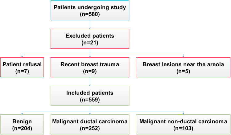
All the patients included in our study underwent an US-guided breast biopsy using an automatic 14G biopsy gun. According to the histopathological results, the patients were divided into three categories: benign lesions (204 cases), ductal carcinomas (252 cases), and non-ductal carcinomas (103 cases), regardless of the type (papillary, lobular, medullary, tubular), obtaining a total of 355 cases of malignant pathology. Cases containing both ductal and non-ductal carcinoma (mixed type) were considered ductal (Fig. 1).

Fig. 1.

Exclusion criteria flow chart

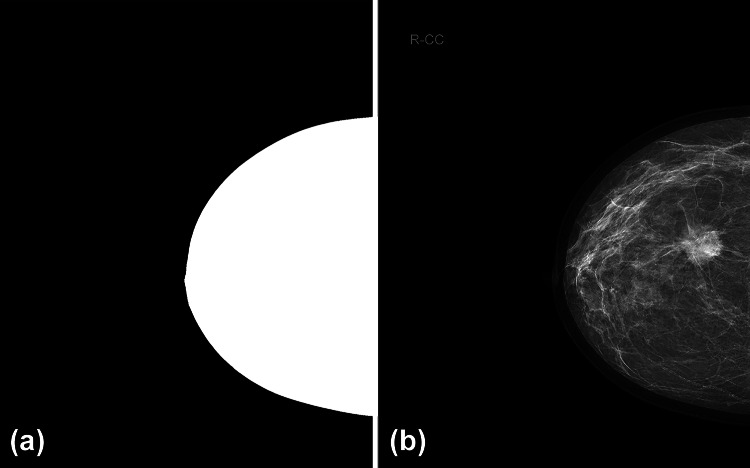
Before training the DL algorithm, the images underwent pre-processing and segmentation stages (removing the nipple, labels, and background area), as mentioned in other studies [6]. These alterations were performed in order to remove all possible artifacts that could alter the classification. Left breast mammograms were mirrored to accurately compare them to the right breast mammograms. Using a threshold, a breast mask was generated (Fig. 2a). Since the breast areola has significant variability in the female population, an algorithm was applied in order to remove it and, in part, the adjacent skin (Fig. 2b).

Fig. 2.

(a) Resulted breast mask. (b) Areola and adjacent skin removal (purple)

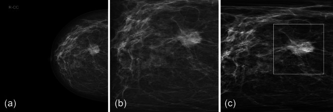
The remaining breast image was resized on the Y axis to a square image. Although the image that was obtained after this operation appears unnatural, the ratios between different grayscale patterns remained similar (Fig. 3a, b). Images were resized to 512 × 512 pixels. A variable square of 322,622 pixels was searched inside each image to identify the most intense average, thus, localizing a high-probability tumor site (Fig. 3c). At this point, each image can be rotated with no information loss, given the fact that ratios between different grayscale aspects were preserved. By applying the rotation, the Thatcher effect can be removed from the learning paradigm [9].

Fig. 3.

(a) Original mammogram. (b) Resized mammogram on the Y axis. (c) Localized tumor

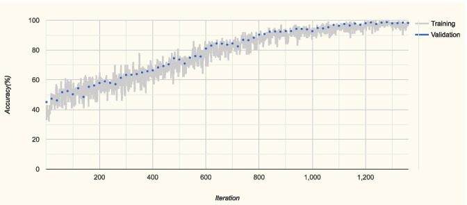
Taking into consideration all the above combined with the need for data augmentation, each image was rotated 360 times and a crop of 227 × 227 pixels was saved, resulting in a total of 201,240 images. The DL algorithm transfer learning was used from AlexNet network [10]. AlexNet is a CNN that is trained on more than a million images from the ImageNet database (available for free on http://www.image-net.org). The network is 8 computing layers deep (Fig. 4) and can classify images into 1000 object categories. The network is linear, having multiple convolutional kernels—filters that extract image features. In each convolutional layer, the kernels have the same size. It has five convolutional layers with different filter sizes: convolutional layer no. 1 has 96 filters of 11 × 11 × 3 convolutions with [4 4] stride and no padding, convolutional layer no. 2 has two groups of 128 filters of 5 × 5 × 48 convolutions with [1 1] stride and [2 2 2 2] padding, convolutional layer no. 3 has 384 filters of 3 × 3 × 256 convolutions with [1 1] stride and [1 1 1 1] padding, convolutional layer no. 4 has 2 groups of 192 filters of 3 × 3 × 192 convolutions with [1 1] stride and [1 1 1 1] padding, and, convolutional layer no. 5 has 2 groups of 128 filters of 3 × 3 × 192 convolutions with [4 4] stride and [1 1 1 1] padding. Additional ReLU, normalization, and max pooling layers are inserted between the first, second, and third convolutional layers, while layers 3, 4, and 5 are followed only by ReLU layers. The rest of the network consists of three fully connected layers, interconnected with ReLU and drop layers that end up in a softmax layer before the classification layer. The different configurations of the non-convolutional layers can be read in the original paper [10]. The network has an input image size of 227 × 227 which is the reason why our images were cropped to this size. A sample of the training sequence is presented in Fig. 5.

Fig. 4.

Layers of AlexNet network

Fig. 5.

Example of training sequence

In order to achieve a suitable statistical power (two-type of null hypothesis with default statistical power goal P ≥ 95% and type I error with 0.05 level of significance), we had to run the network 100 times [11]. We have used the standard tenfold cross-validation, each time the training, validation, and test images were randomly selected and presented in a different order. At each network run, a constant 80, 10, and 10 percentages were used for training, validation, and testing, respectively. The number of epochs was empirically set to 4, but the training sessions usually ended before the second or third epoch when the validation criterion was met.

We reported the testing performance for the classification tasks using the AUC and ACC. The resulted mean and standard deviation values are presented.

In order to assess the performance of the model, we have compared its accuracy with the ones of two radiologists. We used the tenfold cross-validation, each time leaving one subset out for testing purposes. We ran the program 30 times, resulting in 30 test sample data. The two radiologists labeled the 30 test sample data also. We were interested in performing a statistical analysis of the accuracies obtained on each test sample by the three competitors. The performances in terms of mean accuracy (ACC) and standard deviation (SD) are presented in Table 1.

Table 1.

Performances of model vs. radiologist 1 vs. radiologist 2

	Mean ACC	SD
Model	99.28	2.24
Radiologist 1	78.03	12.12
Radiologist 2	72.85	13.50

The algorithm and the statistical evaluation were carried out in MATLAB (MathWorks USA, www.mathworks.com/products/matlab.html).

Results

A new computer application capable of histological breast tumor classification from MM was created.

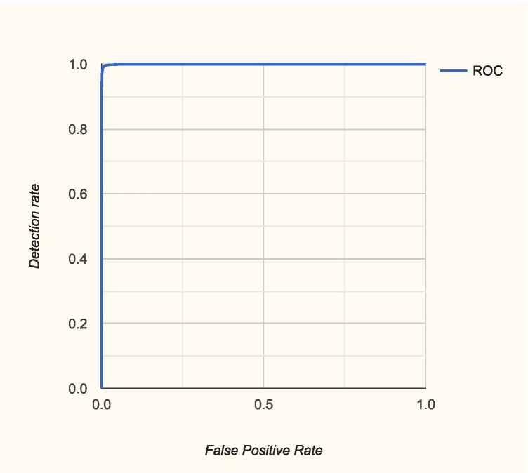
The mean and standard deviation for the ACC was 95.8344% ± 6.3720% and for AUC was 0.9910% ± 0.0366%, computed on 100 runs of the algorithm. The ROC curve and the confusion matrix from the same run are presented in Fig. 6 and Table 2.

Fig. 6.

Example of ROC curve

Table 2.

Confusion matrix on a random run with 95.03% ACC

Output classes	Benign	6043 35.3%	359 2.1%	104 0.6%	92.9% 7.1%
	Ductal	159 0.9%	7259 42.4%	95 0.6%	96.6% 3.4%
	Non-ductal	40 0.2%	93 0.5%	2953 17.3%	95.7% 4.3%
		96.8% 3.2%	94.1% 5.9%	93.7% 6.3%	95.0% 5.0%
		Benign	Ductal	Non-ductal
		Target classes

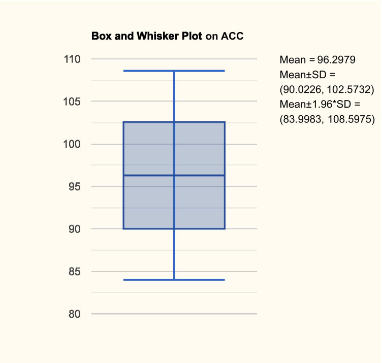
The evaluation of different machine learning algorithms in fair terms needs a standard methodology. A set of benchmarking rules is crucial to improve the quality of our results. Therefore, a statistical assessment is imperative. Hence, the algorithm has been executed in 100 different computer runs, obtaining a statistical power that equals 99% with type I error α = 0.05 for the statistical test that have used. Consequently, the algorithm has been run 100 times in a complete cross-validation cycle using the tenfold cross-validation method. In Fig. 7, we have the box and whisker plot on ACC.

Fig. 7.

Box and whisker plot on ACC

We can see from Fig. 7 that the model is not very stable, since the SD is 6.37. Thus, we can state that the machine learning model cannot offer omnibus robustness.

Next, we have studied the normality of the performance results using the Kolmogorov–Smirnov and Lilliefors test and the Shapiro–Wilk test. We have used the first test because we can compute the mean and SD from the actual data, and the second because it has better power properties. It is worth to mention that in this case the distribution of data is nearly Gaussian, whatever the test results and the distribution of the values, since the sample size corresponds to 100 computer runs. As the sample size increases above 30, the central limit theorem states that the distribution becomes normal.

From Table 3, we can see that the p-level given by the Kolmogorov–Smirnov and Lilliefors test is < 0.1, meaning that indeed the sample size is normally distributed, but the p-level given by the Shapiro–Wilk test is < 0.05; hence, there are significant differences between the sample’s distribution and the Gaussian distribution. Fortunately, as stated above, we can presume the normality due to the central limit theorem.

Table 3.

Statistical assessment of the algorithm’s ACC

Variable	Kolmogorov–Smirnov	Lilliefors p	Shapiro–Wilk	p-level
DL ACC	0.328	0.1	0.372	0.000

We have also computed the skewness = 5.16, and kurtosis = 28.23, that prove once again that it is crucial to run the model 100 times in order to obtain reliable results.

From Table 1, we can see that the model outperforms the two radiologists, in terms of accuracy, and it also is more robust, the SD being 2.24.

Since the statistical tests used in the benchmarking process are based on the assumption that the sample data is governed by the normal distribution, first we applied normality tests to see whether the accuracies are normally distributed or not. Note that we are testing the distribution of data regarding the performances, not the actual data that the algorithm has been tested on. Hence, we have applied the Kolmogorov–Smirnov and Lilliefors test and the Shapiro–Wilk W test, the results being described in Table 4.

Table 4.

Normality tests

	K-S	p-level	Lilliefors p	S-W W	p-level
Model	0.517	< 0.01	< 0.01	0.365	0.000
Radiologist 1	0.200	< 0.05	< 0.01	0.863	0.001
Radiologist 2	0.205	< 0.15	< 0.01	0.956	0.280

From Table 4, we can see that the data is not normally distributed; only the Shapiro–Wilk W test for radiologist 2 states that the data is Gaussian. Nevertheless, having the sample size of 30, due to the central limit theorem, we can say that the data is approximately normal.

The contrast between the model’s performance and the performance of the two radiologists can be statistically measured using the one-way ANOVA technique. The one-way ANOVA results regarding the sum of squares (SS), degrees of freedom (df), mean squares (MS), F-value, and p-level (contrast quadratic polynomial) are presented in Table 5. It can be easily seen that there are significant differences in the classification performances (p-level < 0.05), thus obtaining a confirmation of the model’s power.

Table 5.

One-way ANOVA

SS	df	MS	F-value	p-level
9024,107	81	111.408	45.29	0.000

Besides the one-way ANOVA, we have performed the t-test for independent variables, to verify two by two the performances. The results are presented in Table 6.

Table 6.

t-test results

	t-value	df	F-ratio	p-level
Model vs. radiologist 1	9.121	54	29.23	0.000
Model vs. radiologist 2	10.218	54	36.26	0.000

As shown in Table 6, there are significant differences in means (p-level < 0.05) between the model and the two radiologists, proving once again its classification performance.

To conclude, all the above tests have provided the confirmation that there are significant statistical differences between the model and the two radiologists, and that the model indeed outperforms the two radiologists.

Discussion

Using transfer learning from AlexNet and multiple pre-processing steps, we have developed an algorithm capable of classifying mammograms into three classes—benign, ductal, and non-ductal carcinoma—with an average ACC around 96 and mean AUC 0.99, taking into consideration only the CC view.

It is a well-known fact that MM has a high sensitivity to detect breast tumors, even ductal carcinoma (linear/multiple clusters of fine granular calcification) but the breast biopsy is the gold standard for diagnosis [12]. Ductal carcinoma is the most common form of breast cancer, representing around 80% of all breast cancer diagnosis, as presented also in our study by the higher number of ductal carcinomas compared to non-ductal [13].

Artificial intelligence (AI) refers to all the techniques which determine computers to mimic human behavior, while ML is a subset of AI, which uses statistical methods to enable machines to improve with experience. DL is considered to be a subset of ML techniques, which provides much better results than ML with CNN [14]. DL has gained performance lately due to increasingly more efficient training methods and amounts of data [7]. An AI-based system matched the cancer detection ACC in over 28,000 breast cancer screening mammograms interpreted by 101 radiologists. The system recorded an AUC higher than over 60% of radiologists specialized in breast imaging. AI systems can also be used as an independent first or second reader in places with a shortage of radiologists, or as a support tool [15].

Human interpretation creates great susceptibility to a subjective assessment. That is why a second reading of a mammogram by a computerized technique can improve the results [16]. Therefore, in clinical use, the sensitivity of the detection of breast masses can be improved with the help of a system which acts like a second opinion, in order to reduce the possibility of missing any breast lesion difficult to be identified through a manual process [17]. An increased variability in terms of lesion shape, texture, and size represents a challenge for radiologists, because a lot of small breast masses can be missed. BI-RADS (Breast Imaging-Reporting and Data System) provides a standardized terminology for masses regarding shape (round/oval/irregular), margins (circumscribed/obscured/microlobulated/indistinct/spiculated), or density (high/equal/low or fat-containing) on mammograms [18]. The breast density can also pose a great challenge for radiologists. A high breast density is associated with an increased risk of proliferative lesions that may be considered precursors of breast cancer. The variations in breast tissue are reflected by the breast density [17, 19]. A high breast density can mask breast tumors, being a well-known fact that the sensitivity of MM is reduced in women with dense breasts [20]. In these cases, supplemental imaging or spot compression is necessary.

Given the total number of cases was only 559, the algorithm must be tested on a larger dataset in order to ensure its stability. With a larger dataset, the non-ductal class can also be divided into different subclasses like lobular, tubular, papillary, or medullary carcinoma, thus offering more information to the oncologist. In order to be taken into consideration for clinical use, AI algorithms need continuous studies and large amounts of data to be trained in order to improve and obtain a better performance. AI is considered to be a real opportunity for the improvement of medical fields, especially for radiology. Being trained continuously with increasing amounts of data, the algorithms manage to provide information about every abnormal finding, by extracting particular features which may or may not be detected by the naked eye. The tumor stage will still play a significant role in the overall survival rates, adjusting therapy decisions and surgical options [21]. The use of AI will inevitably find itself implemented in medical fields and distrust of this new technology will not stop its adherence in medical sciences.

Routine views in mammography exploration are bilateral CC and MLO views [22]. Similar with the necessity of the lateral view of the chest X-ray that complements the frontal view, the two images are needed to better understand the position of the object(s) of interest related to the surrounding context. As the images represent the plane projection of a 3-dimensional structure (volume) and overlapping components are hard to individualize, especially when the margins are superposed or when a much denser (intense) object covers other objects. Although the MLO view is the more important projection [23, 24] as it allows visualization of most breast tissue, we decided to only include the CC view in our study because the images are more homogenous compared to the MLO views which have a higher degree of variability as the axilla and pectoral muscles are included. Thus, the study has innate limitations, as the CC view cannot identify posterior breast lesions adjacent to the pectoral muscle. Nevertheless, the research does not aim tumor position, only tumor classification.

Conclusion

Based on the results, the proposed solution can be used as a non-invasive and highly accurate computer-aided system based on DL that can classify breast lesions based on changes identified on mammograms in the CC view. The proposed DL algorithm may be used as an objective first or second reader and as a support tool to accelerate radiologist’s processing time for examination in order to reduce the morbimortality of breast cancer and allow a faster and more effective treatment.

Abbreviations

ACC

Accuracy

DL

Deep learning

ML

Machine learning

AI

Artificial intelligence

CNN

Convolutional neural network

MM

Mammography

MLO

Medio-lateral oblique

CC

Cranio-caudal

BI-RADS

Breast Imaging-Reporting and Data System

Author Contribution

REN, MSS, and IAG share main authorship due to conceiving the main conceptual ideas and designing the study. GCC and REN performed all the imaging techniques and ultrasound-guided breast biopsies. MSS designed the model and the computational framework and with support from CTS and LMF carried out the implementation and worked out all the technical details. IAG supervised the study and together with the rest of the authors provided critical feedback and helped shape the research, analysis, and manuscript.

Availability of Data and Material

Due to the nature of this research, participants of this study did not agree for their data to be shared publicly.

Code Availability

The code used in this study is available from the corresponding author, MSS, upon reasonable request.

Declarations

Ethics Approval

Institutional review board approval was obtained (University of Medicine and Pharmacy of Craiova, Committee of Ethics and Academic and Scientific Deontology approval 45/17.06.2020).

Consent to Participate

Written informed consent was obtained from all subjects (patients) in this study.

Conflict of Interest

The authors declare no competing interests.

References

- 1.Iacoviello L, Bonaccio M, de Gaetano G, Donati MB: Epidemiology of breast cancer, a paradigm of the “common soil” hypothesis. Semin Cancer Biol, 10.1016/j.semcancer, February 20, 2020 [DOI] [PubMed]
- 2.Gheonea IA, Donoiu L, Camen D, Popescu FC, Bondari S. Sonoelastography of breast lesions: A prospective study of 215 cases with histopathological correlation. Rom J Morphol Embryol. 2011;52:1209–1214. [PubMed] [Google Scholar]
- 3.Gheonea IA, Stoica Z, Bondari S. Differential diagnosis of breast lesions using ultrasound elastography. Indian J Radiol Imaging. 2011;21:301–305. doi: 10.4103/0971-3026.90697. [DOI] [PMC free article] [PubMed] [Google Scholar]
- 4.Donoiu L, Camen D, Camen G, Calota F: A comparison of echography and elastography in the differentiation of breast tumors. Ultraschall Med – Eur J Ultrasound 29:OP_2_5,2008
- 5.Shen L, Margolies LR, Rothstein JH, Fluder E, McBride R, Sieh W. Deep Learning to Improve Breast Cancer Detection on Screening Mammography. Sci Rep. 2019;9:1–2. doi: 10.1038/s41598-019-48995-4. [DOI] [PMC free article] [PubMed] [Google Scholar]
- 6.Abdelhafiz D, Yang C, Ammar R, Nabavi S. Deep convolutional neural networks for mammography: Advances, challenges and applications. BMC Bioinformatics. 2019;20:281. doi: 10.1186/s12859-019-2823-4. [DOI] [PMC free article] [PubMed] [Google Scholar]
- 7.Kooi T, Litjens G, Van Ginneken B, Gubern-Mérida A, Sánchez CI, Mann R, den Heeten A, Karssemeijer N. Large scale deep learning for computer aided detection of mammographic lesions. Med Image Anal. 2017;35:303–312. doi: 10.1016/j.media.2016.07.007. [DOI] [PubMed] [Google Scholar]
- 8.Hayes Balmadrid MA, Shelby RA, Wren AA, Miller LS, Yoon SC, Baker JA, Wildermann LA, Soo MS. Anxiety prior to breast biopsy: Relationships with length of time from breast biopsy recommendation to biopsy procedure and psychosocial factors. J Health Psychol. 2017;22(5):561–571. doi: 10.1177/1359105315607828. [DOI] [PubMed] [Google Scholar]
- 9.Thatcher effect. Available at https://en.wikipedia.org/wiki/Thatcher_effect. Accessed 12 June 2020
- 10.AlexNet convolutional neural network – MATLAB alexnet. Available at https://uk.mathworks.com/help/deeplearning/ref/alexnet.html. Accessed 10 June 2020
- 11.Belciug S. Artificial Intelligence in cancer, diagnostic to tailored treatment. 1. Cambridge Massachusetts: Academic Press; 2020. [Google Scholar]
- 12.Venkatesan A, Chu P, Kerlikowske K, Sickles E, Smith-Bindman R. Positive predictive value of specific mammographic findings according to reader and patient variables. Radiology. 2009;250:648–657. doi: 10.1148/radiol.2503080541. [DOI] [PMC free article] [PubMed] [Google Scholar]
- 13.Invasive Ductal Carcinoma (IDC). Available at https://www.hopkinsmedicine.org/breast_center/breast_cancers_other_conditions/invasive_ductal_carcinoma.html#:~:text=Invasive%20ductal%20carcinoma%20(IDC)%2C,of%20all%20breast%20cancer%20diagnoses. Accessed 12 June 2020
- 14.Artificial Intelligence, Machine Learning & Deep learning. Available at https://becominghuman.ai/artificial-intilligence-machine-learning-deep-learning-df6dd0af500e. Accessed 12 June 2020
- 15.Rodriguez-Ruiz A, Lång K, Gubern-Merida A, Broeders M, Gennaro G, Clauser P, Helbich TH, Chevalier M, Tan T, Mertelmeier T, Wallis MG. Stand-Alone Artificial Intelligence for Breast Cancer Detection in Mammography: Comparison With 101 Radiologists. JNCI J Natl Cancer Inst. 2019;111:916–922. doi: 10.1093/jnci/djy222. [DOI] [PMC free article] [PubMed] [Google Scholar]
- 16.Dhungel N, Carneiro G, Bradley AP. A deep learning approach for the analysis of masses in mammograms with minimal user intervention. Med Image Anal. 2017;37:114–128. doi: 10.1016/j.media.2017.01.009. [DOI] [PubMed] [Google Scholar]
- 17.Institute of Electrical and Electronics Engineers, International Association for Pattern Recognition, Australian Pattern Recognition Society: Automated Mass Detection in Mammograms using Cascaded Deep Learning and Random Forests. Available at https://cs.adelaide.edu.au/~carneiro/publications/mass_detection_dicta.pdf. Accessed 10 June 2020
- 18.Breast Imaging-Reporting and Data System (BI-RADS). Available at https://radiopaedia.org/articles/breast-imaging-reporting-and-data-system-bi-rads. Accessed 21 July 2021
- 19.Boyd NF, Martin LJ, Bronskill M, Yaffe MJ, Duric N, Minkin S. Breast tissue composition and susceptibility to breast cancer. J Natl Cancer Inst. 2010;102:1224–1237. doi: 10.1093/jnci/djq239. [DOI] [PMC free article] [PubMed] [Google Scholar]
- 20.Kerlikowske K, Zhu W, Tosteson AN, Sprague BL, Tice JA, Lehman CD, Miglioretti DL. Identifying Women With Dense Breasts at High Risk for Interval Cancer: A Cohort Study. Ann Intern Med. 2015;162:673–681. doi: 10.7326/M14-1465. [DOI] [PMC free article] [PubMed] [Google Scholar]
- 21.Merino Bonilla JA, Torres Tabanera M, Ros Mendoza LH. Breast Cancer in the 21st Century: From Early Detection to New Therapies. Radiologia. 2017;59:368–379. doi: 10.1016/j.rx.2017.06.003. [DOI] [PubMed] [Google Scholar]
- 22.Mammography views. Available at https://radiopaedia.org/articles/mammography-views. Accessed 21 July 2021
- 23.Cogan T, Tamil L. Deep Understanding of Breast Density Classification. Annu Int Conf IEEE Eng Med Biol Soc. 2020;1140–1143:2020. doi: 10.1109/EMBC44109.2020.9176628. [DOI] [PubMed] [Google Scholar]
- 24.Mohamed AA, Luo Y, Peng H, Jankowitz RC, Wu S. Understanding Clinical Mammographic Breast Density Assessment: a Deep Learning Perspective. J Digit Imaging. 2018;31(4):387–392. doi: 10.1007/s10278-017-0022-2. [DOI] [PMC free article] [PubMed] [Google Scholar]
Associated Data
This section collects any data citations, data availability statements, or supplementary materials included in this article.
Data Availability Statement