

Abstract
The process of treating brain cancer depends on the experience and knowledge of the physician, which may be associated with eye errors or may vary from person to person. For this reason, it is important to utilize an automatic tumor detection algorithm to assist radiologists and physicians for brain tumor diagnosis. The aim of the present study is to automatically detect the location of the tumor in a brain MRI image with high accuracy. For this end, in the proposed algorithm, first, the skull is separated from the brain using morphological operators. The image is then segmented by six evolutionary algorithms, i.e., Particle Swarm Optimization (PSO), Artificial Bee Colony (ABC), Genetic Algorithm (GA), Differential Evolution (DE), Harmony Search (HS), and Gray Wolf Optimization (GWO), as well as two other frequently-used techniques in the literature, i.e., K-means and Otsu thresholding algorithms. Afterwards, the tumor area is isolated from the brain using the four features extracted from the main tumor. Evaluation of the segmented area revealed that the PSO has the best performance compared with the other approaches. The segmented results of the PSO are then used as the initial curve for the Active contour to precisely specify the tumor boundaries. The proposed algorithm is applied on fifty images with two different types of tumors. Experimental results on T1-weighted brain MRI images show a better performance of the proposed algorithm compared to other evolutionary algorithms, K-means, and Otsu thresholding methods.
Keywords: Tumor detection, Morphological operators, Evolutionary algorithms, K-means, Otsu thresholding algorithm, Active contour
Introduction
A brain tumor is a collection or mass of abnormal cells in the brain which can be divided into benign and malignant. The tumor may be located in different parts of the brain, and it can be in different sizes and types. The best method which is mostly common for the diagnosis of brain tumors is magnetic resonance imaging (MRI). MRI is an appropriate method that exploits the properties of magnetism and radio waves, and it is highly popular for the diagnosis of various diseases. This method is more suitable and less dangerous than the other imaging approaches due to its features, such as the use of ionizing radiation, very low disturbances, the ability to penetrate without weakening the bones, and the ability to shoot from any desired section [1].
Image segmentation is the first and the most critical stage of image processing which aims to extract valuable information from an image. Tumor treatment depends on the type, size, and location of the tumor [2]. There exist numerous challenges associated with brain tumor detection. Brain tumors can be found in any size, intensity, and shape, and they can be located in any location of the MRI brain images. Some tumors also deform into other structures and appear with edema that alters the intensity of the pixels in the area surrounding them [3]. It is important to carefully choose the right method of segmentation because a small error can cause major problems in the surgery. The performance of most of the segmentation methods is adversely affected by the presence of noise and heterogeneity in the brightness of the MRI image. In addition, their performance is usually restricted due to their high computational cost, high complexity, and low accuracy of the segmentation. A traditional way to segment brain images is to use the experience of a specialist physician to manually determine the boundaries of the area of interest in brain images.
There are three types of image segmentation techniques: manual, semi-automatic, and automatic segmentation. Manual segmentation seems to be the first choice; however, due to the low contrast of the tissues, the lack of clarity of borders, the lack of hand–eye coordination, and its time-consuming nature, this type of segmentation is not recommended nowadays [4]. The semi-automatic techniques are comprised of the user interaction and software processing steps [5]. Nonetheless, the disadvantage of this method is the necessity of using expert users for the final segmentation which is also time-consuming. Henceforth, utilizing an automatic tumor detection approach is valuable and it is extensively used for the segmentation of brain tumor [5, 6].
Automatic tumor detection is usually performed in three steps: pre-processing, segmentation, and post-processing.
Pre-processing
Before starting the segmentation process, any unwanted artifacts should be removed from the MRI image. Pre-processing includes several steps: converting the image to grayscale, noise reduction, and image enhancement. Moreover, for medical images, such as brain images, it might be necessary to remove the skull region from the MRI brain image as well.
Skull stripping has played an important role as a preliminary step for the segmentation which can be challenging because of the complexity of the human brain and the variation of the parameters of the MRI scanners. Park and Lee [7] removed the skull region from the MRI brain images using the region growing algorithm. They first exploited histogram analysis for eliminating the background voxels, and then two seed regions of the brain and non-brain regions were automatically identified using a mask produced by morphological operators. Then, general brain anatomy information was used to expand these seed regions using a 2D region growing algorithm. Mathematical morphology (e.g., erosion and dilation) is an attractive technique for skull stripping since it is fast and easy to implement. Brummer et al. [8] used histogram analysis and morphological operations for skull stripping. Chiverton et al. [9] eliminated the skull region using a combination of mathematical morphological operations and statistical techniques.
Segmentation
Image segmentation is a process in which the image is divided into multiple separated homogeneous areas. So, the sum of these separated regions is equal to the whole image and these areas have no overlap with each other [10]. There are numerous techniques for image segmentation. One of the well-known methods is K-means algorithm. K-means is an unsupervised clustering method that is used to identify clusters of data objects in a dataset. Vijay and Subhashini [11] combined segmentation and K-means clustering to extract the tumor from the MRI brain image. They compared the performance of their proposed technique with other clustering methods. Less execution time was achieved by their method compared to the other clustering methods [11]. However, the performance of this algorithm highly depends on the initial selection of the cluster centroids and it might not converge to the optimum result. The histogram-based segmentation method is another effective tool for image segmentation which only requires one passage between the pixels for the segmentation purpose [12–15]. In this method, a histogram is calculated based on all the pixels in the image and the peaks and valleys in the histogram are used to place cluster boundaries at these regions of the image. Akter et al. [16] defined a threshold value based on the maximum peak of the histogram of the cancerous hemisphere. Then, the pixels with values less than the threshold were removed. Afterwards, the median filtering was applied to reduce the randomness of the pixels, and finally, the largest cluster was selected as the tumor. One of the interesting methods, which are based on the image histogram, is Otsu thresholding algorithm which is an automatic image thresholding method. It returns a single intensity value to divide the image into two classes in its simplest form. The threshold is determined by minimizing intra-class intensity variance, or equivalently, by maximizing inter-class variance [17]. Zhang et al. [18] used a new thresholding algorithm based on multiscale 3D Otsu for medical image segmentation. They reported that 3D Otsu can provide more precise segmentations comparing to 1D Otsu because of its capability of incorporating spatial information. One of the disadvantages of histogram-based methods is that they may not be able to accurately find peaks and valleys in low-contrast images [19, 20].
Social intelligence is a type of artificial intelligence based on social behaviors where the members interact locally with each other and with their environment simultaneously [21]. Evolutionary algorithms are also a kind of population-based random search, and their most important strength is their ability to explore the search space in parallel and in different directions. In these methods, because the search space is explored comprehensively, they less likely get stuck in local minima. Particle Swarm Optimization (PSO) simulates the social behavior of bird flocking, and it is based on social intelligence. Benaichouche et al. [22] used the PSO algorithm to optimize the segmentation results obtained from the FCM method. Sharif et al. [23] used PSO algorithm for segmentation along with a classifier to precisely extract the tumor from MRI images of the brain. Indeed, they first removed the skull area by the Brain Surface Extractor (BSE) which is a skull stripping tool, and the image was then divided by the PSO algorithm. In the next step, Local Binary Patterns (LBP) and image properties were extracted. Next, the Genetic Algorithm (GA) was used to extract the best features. Finally, the Artificial Neural Network (ANN) was applied to classify the tumor. Vijay et al. [24] applied Enhanced Darwinian Particle Swarm Optimization (EDPSO) for automated tumor detection, and the classification was performed by the Adaptive Neuron-Fuzzy Inference System. The Artificial Bee Colony (ABC) is also an evolutionary algorithm based on the behavior of honeybees. Hancer et al. [25] employed the ABC algorithm to detect brain tumors. First, the ABC algorithm was used for the segmentation purpose, and then, a thresholding method was applied for the tumor isolation. Cuevas et al. [26] applied the ABC algorithm to compute the threshold value for image segmentation. Histogram of an image was approximated through a Gaussian mixture model where its parameters were estimated by the ABC algorithm. Khorram and Yazdi [27] proposed an optimized thresholding method for segmentation of MRI brain images and tumor detection using the Ant Colony Optimization(ACO) algorithm. In their work, textural features were adopted as heuristic information. The results of the evaluation criteria of their proposed algorithm were better than those of other evolutionary algorithms; however, in the case of tumor detection, the values obtained from different evaluation criteria were not high enough [27]. Taherdangkoo et al. [28] also provided a method for MRI brain segmentation based on the ACO algorithm. The obtained results demonstrated high converging rate and accuracy. GA is another evolutionary algorithm which is widely used for tumor detection [2, 29]. Bahadure et al. [30] compared different segmentation techniques for tumor detection and picked the best one by comparing their segmentation score. Based on their report, BWT-based segmentation was the best algorithm in term of performance. Further, they suggested to improve the classification accuracy by using the GA.
In addition to conventional approaches, researchers today utilize advanced techniques for image segmentation, such as model-based segmentation and multivariate segmentation [31]. The Active contour model (also called snakes) is a deformable model that was first introduced by Kass [32]. This model is one of the most admired methods in medical image processing, especially in images with unclear boundaries. This model uses energy constraints to extract the desired area. The idea is based on a flexible curve (or surface) that dynamically matches the required edges or objects in the image, and is controlled by forces applied to it. The energy performance of snakes is the sum of their external and internal energies. This method is widely used in many recent research works [31, 33, 34] for brain tumor segmentation. Shivare et al. [35] used a combination of Active contour model and convex hull for automated brain tumor segmentation. In the first step of their proposed algorithm, a coarse estimation of the brain tumor was carried out using the convex hull approach. Then, the obtained result was employed as the initialization for the Active contour model.
Since evolutionary algorithms have the ability to explore extensively in the search space and less likely get stuck in the local minima, they can be exploited to segment complex images. In general, these algorithms can obtain the tumor area well, but they might not perform well in finding tumor edges in low-contrast images. Due to the fact that in many tumor images the boundary between the tumor and the background is not clear, it is better to use them as an initial step for the image segmentation and then exploit their segmented result as an initial curve for Active contour to more precisely obtain the edges of the tumor.
Post-processing
After the segmentation process, a post-processing should be accomplished to precisely detect the tumor area. Post-processing is a step to refine the nearly exact size, shape, and location of the tumor. It may also include different optimization techniques to further enhance the segmentation results. Akram and Usman [36] applied morphological operations and tumor masking for removing the false segmented pixels after the initial segmentation. Nevertheless, this method might not work for complex images with low-contrast boundaries.
Proposed Method
Figure 1 provides the flow diagram of the proposed algorithm. In the first sub-section, the pre-processing step (i.e. skull stripping) is explained in details. Then, six evolutionary algorithms and two frequently-used non-evolutionary algorithms, i.e., K-means and Otsu thresholding algorithms, are fully described for the initial segmentation of the MRI brain image. In the next step, in order to extract the tumor from the segmented images, four tumor features, two features are related to the features of the tumor mask and the rest are related to the features of the original tumor, are extracted from 100 different brain MRI images. The best algorithm in terms of performance is then chosen and its result is used as an initial curve for the Active contour method for further improvement of the tumor boundaries. The proposed algorithms are applied on 50 MRI images with different types of tumor.
Fig. 1.
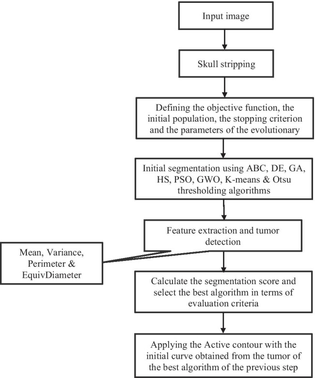
Flow diagram of the proposed algorithm
Skull Stripping
In the first step, after converting the image into a binary image, the opening operator with a disk structuring element is applied on the image to make sure that the skull and brain are not connected anymore. The opening operation erodes an image and then dilates the eroded image. The opening operation is beneficial for removing tiny objects from an image while preserving the shape and the size of the larger objects in the image. After that, the largest element of the image, i.e., the brain tissue, is selected. Next, the closing operator is applied to make sure the lost parts of the brain are reconstructed. The closing operation first dilates an image and then erodes the dilated image using the same structuring element. It is effective for filling small holes of an image while preserving the shape and the size of the objects in the image. At the end, the final mask is multiplied to the original image, which results in an image of the brain without the skull part. The different steps of skull stripping are depicted in Fig. 2.
Fig. 2.

Results of skull stripping: a the original image, b opening operator, c largest element extraction, d closing operator, and e brain after removing the skull
Initial Segmentation
In this sub-section, two frequently-used non-evolutionary algorithms, i.e., K-means and Otsu thresholding, and six evolutionary algorithms for the initial image segmentation are described in details.
K-Means Algorithm
K-means is an iterative clustering method that attempts to segment a set of data in a way that the total distance between the data within the cluster and the center of the cluster is minimized. The K-means algorithm consists of two steps [37]:
- Assignment step: It assigns each data (A) to the cluster with the nearest cluster centroid:
where Ci(t) is cluster i and mi(t) is the center of cluster i.1
-
2.
Updating step: The centroid of each cluster is recalculated and considered as the mean value of the cluster’s member data.
| 2 |
These two steps are repeated until the final result is obtained. There is no guarantee that this algorithm will converge to the optimal clustering as its performance highly depends on the selection of the initial centers of the clusters [38, 39].
In this section, the image is divided into four parts using K-means. In fact, the goal is to find four cluster centers in the image that segment the image in the best way. The stopping criterion in this algorithm is that the center of the clusters must be fixed in five consecutive repetitions.
Otsu Thresholding Algorithm
Otsu thresholding algorithm is mainly used for automatic thresholding in machine vision and image processing. In its simplest form, the algorithm returns a single intensity threshold that separates pixels into two classes, i.e., foreground and background. This threshold is determined by minimizing the variance of the intensity within the clusters, or its equivalent, by maximizing the variance between clusters. In this work, the image is divided into four parts using the Otsu thresholding algorithm.
Particle Swarm Optimization
In order to segment the images, the PSO algorithm is applied to find the best cluster centers for the segmentation. For digital images, pixel intensity levels are considered as particles and they are candidate solutions for the image segmentation. These particles move in each iteration to find the best local neighborhood and global solutions by sharing information with each other and interacting with neighborhood particles. In PSO, a cost function is evaluated after each iteration. The and denote the best previous position encountered by the ith particle and the global best position respectively; also, t denotes the iteration counter. The current velocity of the dth dimension of the ith particle and the new position of the particle are given in Eqs. 3 and 4, respectively.
| 3 |
| 4 |
where , , and are the parameters that assign weights to the individual best, global best, and inertial influence when new velocity is calculated. Stochastic variables and are random numbers between 0 and 1. Clerc and Kennedy [40] obtained the optimal values of the PSO algorithm parameters by conducting several experiments, which these values make a balance between the two concepts of exploitation and exploration. The obtained values for , , and are 0.7289, 1.4962, and 1.4962, respectively. These values have been utilized in our work. The initial particle number is assumed to be 100 for all evolutionary algorithms, which is a fair comparison and reduces the possibility of getting stuck at the local minima. In our work, the objective function is defined as the Euclidean distance within the cluster and the goal is to minimize it.
| 5 |
| 6 |
where is the ith pixel in the dataset, is the jth cluster center, and is the space dimension. The original images have been transformed into one-dimensional arrays. In the first step, the image is divided into four (clusters) by PSO algorithm. The objective function, i.e., the Euclidean distance within the cluster, should be minimized and is defined as follow:
| 7 |
The stopping criterion of the algorithm is that the best cost must remain constant in 15 consecutive repetitions.
Artificial Bee Colony
The ABC algorithm is an optimization algorithm based on the intelligent feeding behavior of bees, introduced by Karaboga and Basturk in 2005 [41]. In this algorithm, each food source is a possible solution to the optimization problem. First, a group of food sources is randomly selected by the bees and the amount of available food in each source is determined. There are three types of bees in the foraging process: employed bees, onlooker bees, and scout bees. An employed bee changes its position by using local information and measuring the objective function. Once the search process is completed by all employed bees, they share the information obtained from the location of their food sources and the amount of food with the onlooker bees. Onlooker bees select a food source after reviewing the obtained information and measuring food levels. An onlooker bee, like an employed bee, corrects its position and moves and examines the amount of food in the new location. If there is more food in the new location, the new location will be replaced by the previous one.
In the implementation of this algorithm, the goal is to find four cluster centers that divide the image into four parts. Similar to the implementation of the PSO algorithm, the initial population is 100. Also, the objective function and the stopping criterion of the algorithm are the same as the work done in the PSO algorithm.
Genetic Algorithm
The GA is an evolutionary method based on Darwin’s theory of evolution. This algorithm starts with a set of answers which are represented by chromosomes. This set of answers is called the initial population. The GA uses the results of one population to generate the next population, and it is hoped that the next population will be better than the previous one. Some of the answers are selected based on their level of competence. The steps of the GA are as follows:
Initial population
Objective function
Selection
Crossover
Mutation
First, the initial population is selected randomly. Each member of the population is called a chromosome. Each chromosome is evaluated by the objective function. The new population is created by selecting the best chromosomes according to their objective function f in the previous iteration. Then, the crossover is applied to generate a new population from the two selected chromosomes, called parents, by exchanging their properties. Afterwards, the mutation is applied to prevent premature convergence by selecting new points randomly. These steps are repeated until the stopping criterion is met. The GA’s predefined parameters used in our work, which were obtained by parameter tuning, are reported in Table 1.
Table 1.
Predefined parameters of the GA
| Parameter | Value |
|---|---|
| Population size (nPop) | 100 |
| Crossover percentage (PC) | 0.8 |
| Number of offsprings (parents) | 2*round (pc*nPop/2) |
| Mutation percentage (PM) | 0.3 |
| Number of mutants | Round (pm*nPop) |
| Mutation rate (mu) | 0.02 |
| Selection pressure | 8 |
The objective function and stopping criterion in this algorithm are similar to the other aforementioned evolutionary algorithms.
Differential Evolution
The DE has high capability in optimization problems in continuous spaces and for nonlinear derivative functions. This algorithm does not have the main drawback of the GA, which is the lack of local search. Unlike the GA in which the chance of choosing an answer as a parent depends on its competency value, in the DE algorithm, all answers have an equal chance of being selected. After selecting an answer using the Mutation and the Crossover operators, this answer is compared to the previous value and replaced if it is better. In this algorithm, unlike other algorithms, the mutation operator is applied before the crossover operator. In order to generate the initial population, this algorithm usually uses a uniform distribution. The members are evenly distributed in the space, and in each iteration of the algorithm, these members come closer to each other to finally achieve convergence and the optimal response. As the number of members increases, it becomes easier to reach the optimal solution. Two important parameters in this algorithm are Beta (the differential weight) and PCR (the crossover probability). In our work, Beta is considered as a random parameter between 0.3 and 0.8 and PCR is considered to be 0.2. The initial population, the objective function, and the stopping criterion are the same as the previous evolutionary algorithms.
Harmony Search
The HS algorithm is inspired by music in order to achieve the best answer. Trying to find this harmony in music is like finding the optimal answer in the optimization process. In fact, the HS algorithm is the best strategy for transforming qualitatively studied processes into quantitative and tangible optimization processes. In this technique, first, some initial harmonies are created to form a harmonious memory (HM). In the next step, some new harmonies are created where the components of these new harmonies are determined from the harmonious memory with a probability of Harmony Memory Considering Rate (HMCR) and are determined randomly with the probability of 1-HMCR. If the component of the new harmonies comes from the HM, it is further mutated according to the Pitching Adjust Rate (PAR). The PAR determines the probability of a candidate from the HM to be mutated. If the new produced harmony is better than the worst harmony in the HM, it will be replaced. This process continues until the algorithm’s stopping condition is met. In our work, the values for the number of the new harmonies, HMCR, and PAR were considered 100, 0.2, and 0.1, respectively.
The initial population, objective function, and stopping criterion of the algorithm are similar to the other proposed evolutionary algorithms.
Gray wolf Optimization Algorithm
The grey wolf optimizer is a novel heuristic swarm intelligent optimization algorithm proposed by Mirjalili et al. in 2014 [42]. This algorithm is inspired by the way gray wolves hunt, and it is in the category of population-based intelligence algorithms. Gray wolves are generally divided into four groups: alpha, beta, delta, and omega. The first, second, and third best individuals are defined as alpha, beta, and delta; the rest are considered as omega. In the optimization process, the locations of the wolves are updated based on Eqs. 8 and 9.
| 8 |
| 9 |
where represents the difference between the position of the prey and predator, shows the current iteration, signifies the prey’s position, and shows the grey wolf’s position. The values of both and can be determined via the following equations:
| 10 |
| 11 |
where the coefficient linearly decreases from 2 to 0 with the increase of iteration number and and are random vectors between 0 and 1.
In reality, the location of the prey is unknown. It always assumes that alpha, beta, and delta positions are likely to be the prey (optimum) position. The first, second, and third best obtained individuals are respectively recorded as alpha (), beta (), and delta (). The other wolves, regarded as omega, relocate their positions according to the locations of alpha, beta, and delta. The following equations are used to re-adjust the position of the wolf omega.
| 12 |
| 13 |
| 14 |
where the values of vectors , , and are set randomly; , and are the positions of alpha, beta, and delta, respectively, and is the position of the current solution.
The final position of the current solution is calculated as follows:
| 15 |
| 16 |
| 17 |
| 18 |
where , , and represent random vectors. The initial population, the objective function, and the stopping criterion, defined in this algorithm, are presented in the same way as in other evolutionary algorithms.
Initial Image Segmentation Using the Eight Proposed Algorithms
In this section, the aim is to segment MRI images of the brain, using the algorithms presented in the previous sections and comparing their performance. The proposed algorithms are applied on 50 images with two different types of tumors (30 MRI brain images contain the Meningioma tumor and 20 MRI brain images contain the pituitary tumor). These two types are different in shape and location. Figure 3 presents the result of the initial segmentation of the MRI brain image containing the Meningioma tumor using GA.
Fig. 3.

a Original image; b initial segmentation using GA
Feature Extraction and Tumor Detection
The segmented image is highly complex, and it is not feasible to detect the tumor from such images using traditional methods, because most of these methods are inefficient for highly complex images. Therefore, an algorithm that is capable to exploit the distinguished features from the segmented regions of the image and uses them to correctly extract the tumor is required. In order to extract the tumor from the segmented regions of images, first, four tumor features are extracted for 100 different images containing the Meningioma tumor. Two of the four features are related to the tumor mask, and the other two are related to the original tumor. The features related to the tumor mask are perimeter and the equivalent diameter, while the other two features are the mean and the variance of the tumor region. The values of these four features are obtained by using 100 different images, and according to the values obtained, it is realized that all the values are in a certain suffering range, and a specific value range for each feature is defined accordingly. Then, all the segmented parts in the initial segmentation of the image are passed through the filter of these features and the tumor areas are selected. This algorithm has a satisfactory result even when the segmented image is extremely complex and the tumor area is invisible from the naked eye.
Improving Tumor Detection Performance by Means of Active Contour
Active contour model is commonly used to extract rich information in medical images. In Active contour model, the initial boundary moves towards an object of interest under the influence of certain forces. One of the limitations of the Active contour model is that the initial boundary must be close enough to the desired area to achieve high accuracy. Therefore, choosing the right initial boundary is essential for fast and accurate access to the desired area. The algorithms proposed in the previous section could well identify the tumor area; however, they perform poorly at precisely finding the tumor boundary. In most of the literature, the initial boundary for the Active contour algorithm is specified manually which cannot be considered as an automatic algorithm. In the present study, the tumor extracted by the best algorithm, in terms of performance, is considered as the initial boundary for the Active contour model. Hereby, the initial boundary which is already good can be refined by Active contour algorithm to achieve more precisely the boundary of the tumor.
Evaluation of MRI Brain Tumor Detection Results
In order to compare the results with ground truth and to evaluate the efficiency of the algorithms, the following parameters are computed:
| 19 |
| 20 |
| 21 |
| 22 |
| 23 |
where FP, FN, TP, and TN denote false positive, false negative, true positive, and true negative, respectively. TP and TN are the number of pixels that are correctly predicted as desirable and undesirable, respectively. On the other hand, FP and FN are the number of pixels that are incorrectly predicted as desirable and undesirable, respectively. Recall is the fraction of the total amount of relevant instances that are actually retrieved. In other words, it is the number of correctly predicted positive results divided by the number of all ground truth positive labels. Precision is the fraction of relevant instances among the retrieved instances. The F-score is a weighted average of the Precision and Recall, so it considers both false positives and false negatives. Accuracy is the fraction of predictions of the model that got right. Jaccard coefficient measures similarity between finite sample sets and is defined as the size of the intersection divided by the size of the union of sample sets.
As evolutionary algorithms may give slightly different results in varied running-times due to random selection of the initial positions, each algorithm was run five times for each image, and the image with the lowest cost function was considered as the output. Then, the mean and the variance of the cost function for these five performances were calculated; finally, the mean of the total variance and the mean of the cost function for 50 images (30 images containing the Meningioma tumor and 20 images containing the pituitary tumor) were obtained to check the reliability of each algorithm.
Results and Discussion
In this section, the results of the initial segmentation of an image using K-means, Otsu thresholding, and the evolutionary algorithms are presented and compared to each other, and then, the best algorithm in terms of performance is utilized for the initial boundary of Active contour for a better segmentation. Two different types of images are used with different tumor types (30 images containing the Meningioma tumor and 20 images containing the Pituitary tumor). The T1-weighted images are provided from [43, 44]. Figure 4 shows the initial segmentation and tumor detection for the Meningioma tumor type using PSO algorithm. Table 2 presents the average evaluation criteria of evolutionary algorithms, K-means, and Otsu thresholding for the Meningioma tumor type on 30 images.
Fig. 4.

Results of the initial segmentation and tumor detection: a original image, b initial segmentation using PSO, c the tumor area recognized by extracted features, and d ground truth
Table 2.
Evaluation of tumor detection performance for the six evolutionary algorithms, K-means, and Otsu thresholding for 30 images containing the Meningioma tumor
| Evaluation criteria | Algorithms | |||||||
|---|---|---|---|---|---|---|---|---|
| ABC | DE | GA | HS | PSO | GWO | K-means | Otsu | |
| Precision | 97.93 | 98.01 | 98.01 | 97.69 | 97.85 | 98.02 | 69.13 | 68.32 |
| Recall | 80.70 | 80.46 | 80.48 | 80.00 | 80.89 | 80.41 | 56.18 | 54.90 |
| F_score | 88.05 | 87.91 | 87.95 | 87.38 | 88.10 | 87.91 | 61.59 | 60.41 |
| Accuracy | 99.54 | 99.54 | 99.54 | 99.52 | 99.55 | 99.54 | 69.68 | 69.63 |
| Jaccard | 79.21 | 79.05 | 79.08 | 78.31 | 79.34 | 79.02 | 55.55 | 53.74 |
The highest value for each metric is shown in bold
All of the steps of the proposed algorithm were applied on 20 images containing the pituitary tumor. Table 3 represents the results of tumor isolation on 20 images for the Pituitary tumor type using evolutionary algorithms, K-means, and Otsu thresholding.
Table 3.
Evaluation of tumor detection performance for the six evolutionary algorithms, K-means, and Otsu for 20 images containing the pituitary tumor
| Evaluation criteria | Algorithms | |||||||
|---|---|---|---|---|---|---|---|---|
| ABC | DE | GA | HS | PSO | GWO | K-means | Otsu | |
| Precision | 96.65 | 95.67 | 95.67 | 95.68 | 95.81 | 95.65 | 92.21 | 77.34 |
| Recall | 84.56 | 84.44 | 84.97 | 83.32 | 85.48 | 84.86 | 79.55 | 67.12 |
| F_score | 89.41 | 89.35 | 89.67 | 88.67 | 90.09 | 89.60 | 85.21 | 71.64 |
| Accuracy | 99.60 | 99.60 | 99.61 | 99.58 | 99.62 | 99.61 | 94.62 | 79.66 |
| Jaccard | 81.12 | 81.02 | 81.54 | 79.96 | 82.21 | 81.43 | 77.51 | 65.08 |
The highest value for each metric is shown in bold
According to Table 2, K-means and Otsu thresholding perform poorly in tumor detection because they cannot find the tumor in 9 out of 30 images. This is due to the fact that the performance of the K-means algorithm is highly dependent on the initial selection of the cluster centers and the algorithm may get stuck at the local minima. In the Otsu algorithm, segmentation is also based on image histogram, and as we need three threshold levels for segmentation, the image histogram should have as many distinct peaks as possible so that the thresholds can be well defined. Meanwhile, in magnetic resonance images, poor contrast exists among the various tissues of the brain. As a consequence, the Otsu algorithm performs poorly in this regard. Recall is one of the most important criteria for evaluating the performance of the algorithms in tumor detection. High Recall indicates that a large number of pixels from tumor region are correctly detected, and this parameter is essential for the surgery of patients with cancer. One hundred percent Recall in the tumor detection means that the entire area of the real tumor is detected by the algorithm, although some parts obtained by the algorithm may not be a tumor. One hundred percent Precision in diagnosing a tumor means that the entire area detected as a tumor by the algorithm is actually a part of the real tumor; however, it may not identify many parts of the real tumor, which may have very dangerous consequences for the surgery. The F-score considers both Recall and Precision criteria for evaluating the performance of algorithms. To evaluate the performance of the algorithms, both Recall and Precision must be considered, but in the case of tumor segmentation, Recall is more important because it considers the entire area of the real tumor. Regarding the performance of GWO and PSO, it is worth to be mentioned that the reason why GWO performs slightly better than PSO only in terms of precision is that GWO has a powerful exploitation procedure (compared to its exploration) which makes it focus on the internal region of the tumor and consequently, increases its precision. However, its bias towards exploitation makes its performance worse than PSO in terms of other evaluation criteria.
According to Tables 2 and 3 and the aforementioned reasons, the performance of PSO algorithm for tumor detection is better than the other techniques.
In addition, since K-means and Otsu algorithms could not find any tumor area in 9 of the images, we discarded these images and we have compared the results of the 21 images that K-means and Otsu algorithms could segment the tumor, with the results of the evolutionary algorithms applied on the same 21 images. Having the results of all the algorithms, it is clear that PSO still has the best performance among all the proposed algorithms (see Tables 4 and 5).
Table 4.
Evaluation of tumor detection performance for the six evolutionary algorithms and K-means in 21 images containing the Meningioma tumor
| Evaluation criteria | Algorithms | ||||||
|---|---|---|---|---|---|---|---|
| ABC | DE | GA | HS | PSO | GWO | K-means | |
| Precision | 98.56 | 98.65 | 98.66 | 98.44 | 98.42 | 98.67 | 98.77 |
| Recall | 81.84 | 81.50 | 81.55 | 81.40 | 82.27 | 81.47 | 80.26 |
| F_score | 88.94 | 88.79 | 88.84 | 88.59 | 89.06 | 88.81 | 87.99 |
| Accuracy | 99.58 | 99.57 | 99.58 | 99.57 | 99.58 | 99.57 | 99.55 |
| Jaccard | 80.75 | 80.51 | 80.57 | 80.20 | 80.93 | 80.50 | 79.37 |
The highest value for each metric is shown in bold
Table 5.
Evaluation of tumor detection performance for the six evolutionary algorithms and Otsu thresholding in 21 images containing the Meningioma tumor
| Evaluation criteria | Algorithms | ||||||
|---|---|---|---|---|---|---|---|
| ABC | DE | GA | HS | PSO | GWO | Otsu | |
| Precision | 97.50 | 97.62 | 97.62 | 97.12 | 97.38 | 97.63 | 97.61 |
| Recall | 84.09 | 83.75 | 83.82 | 83.79 | 84.54 | 83.80 | 78.44 |
| F_score | 90.01 | 89.82 | 89.88 | 89.60 | 90.10 | 89.87 | 86.31 |
| Accuracy | 99.60 | 99.59 | 99.60 | 99.59 | 99.60 | 99.60 | 99.48 |
| Jaccard | 82.23 | 82.01 | 82.08 | 81.61 | 82.45 | 82.08 | 76.78 |
The highest value for each metric is shown in bold
Table 6 reports the mean value and the variance of the cost function over 150 runs per algorithm for 30 images containing the Meningioma tumor.
Table 6.
Comparison of the variance and the mean of the cost function for six evolutionary algorithms containing the Meningioma tumor
| Parameters | Algorithms | |||||
|---|---|---|---|---|---|---|
| ABC | DE | GA | HS | PSO | GWO | |
| Variance | 7.6354 | 21.2720 | 1.1286 | 137.9296 | 0.0011 | 9.4608 |
| Mean | 481.9238 | 484.2254 | 479.8022 | 497.6704 | 479.6766 | 482.1300 |
The highest value for each metric is shown in bold
The very low variance of the results of PSO algorithm proves its reliability and represents that this method rarely gets stuck in the local minima. Also, the mean of the cost function in this algorithm is lower than that for other algorithms, which shows the superiority of PSO over them (see Table 6). The mean and the variance of the cost function in the hundred times run of each algorithm for pituitary tumor are reported in Table 7.
Table 7.
Comparison of the variance and the mean of the cost function for six evolutionary algorithms containing the pituitary tumor
| Parameters | Algorithms | |||||
|---|---|---|---|---|---|---|
| ABC | DE | GA | HS | PSO | GWO | |
| Variance | 5.0861 | 17.0320 | 4.4364 | 244.0903 | 2.35 × 10⁻⁸ | 7.9893 |
| Mean | 447.3164 | 450.0634 | 445.9285 | 466.9992 | 445.9148 | 448.3082 |
The highest value for each metric is shown in bold
All the results obtained in both types of tumors show the superiority of the PSO algorithm over other algorithms.
After comparing the results of the mentioned algorithms and evaluating the defined comparison criteria, the PSO algorithm had the best performance among the other algorithms. Nevertheless, to achieve a higher accuracy, it is required to use an algorithm which is able to obtain the edges of the tumor more accurately. The Active contour algorithm can perform very well but it is highly dependent on the initial boundary. Henceforth, the tumor area detected by the PSO algorithm is used as an initial boundary for the Active contour model. Figure 5 shows the results of tumor detection from a MRI brain image using Active contour with an initial boundary obtained by PSO algorithm for both types of tumors. We call this combination as our proposed algorithm. Rows 1 to 3 in Fig. 5 depict the images containing the pituitary tumor, and rows 4 to 6 show the images containing the Meningioma tumor. The results of PSO algorithm and our proposed algorithm for 30 images containing the Meningioma tumor are presented in Table 8. All the evaluation criteria computed for the proposed algorithm, except Precision, have been significantly increased, which shows that the proposed algorithm has a higher ability to obtain tumor edges than the PSO. The high Precision of PSO algorithm is due to the fact that the algorithm has obtained the area inside the tumor, so it has a low FP, and as a result, the Precision has been increased according to its formula. However, since this algorithm has performed poorly in obtaining the edges, the FN is very high which results in a very low Recall and other evaluation criteria. Figure 6 shows the results of tumor detection on MRI brain images containing the Meningioma tumor using different algorithms. Figure 7 shows the same results on MRI brain images containing the Pituitary tumor.
Fig. 5.

Tumor detection results for both types of tumors: a original images, b initial segmentation using PSO algorithm, c tumor area by means of PSO, d the proposed algorithm, and e ground truth
Table 8.
Comparison of tumor detection performance in PSO algorithm and proposed algorithm in 30 images containing the Meningioma tumor
| Evaluation criteria | Algorithms | |
|---|---|---|
| PSO | Proposed algorithm | |
| Precision | 97.85 | 94.67 |
| Recall | 80.89 | 94.13 |
| F_score | 88.10 | 94.24 |
| Accuracy | 99.55 | 99.76 |
| Jaccard | 79.34 | 89.21 |
The highest value for each metric is shown in bold
Fig. 6.

Results of tumor detection on a MRI brain image containing the Meningioma tumor: a original image, b ABC, c DE, d GA, e HS, f GWO, g PSO, h) the proposed algorithm, and i ground truth
Fig. 7.

The results of tumor detection on a MRI brain image containing the pituitary tumor: a original image, b ABC, c DE, d GA, e HS, f GWO, g PSO, h the proposed algorithm, and i ground truth
Table 9 shows the performance evaluation of the proposed algorithm and PSO for 20 MRI images containing the pituitary tumor.
Table 9.
Comparison of tumor detection performance in PSO algorithm and proposed algorithm in 20 images containing the pituitary tumor
| Evaluation criteria | Algorithms | |
|---|---|---|
| PSO | Proposed algorithm | |
| Precision | 95.81 | 93.69 |
| Recall | 85.48 | 91.95 |
| F_score | 90.09 | 92.62 |
| Accuracy | 99.62 | 99.72 |
| Jaccard | 82.21 | 86.46 |
The highest value for each metric is shown in bold
According to Table 9, the accuracy, Recall, F-score, and Jaccard of the proposed algorithm are much higher than those of the other evolutionary methods, K-means, and Otsu thresholding. As mentioned above, high Precision indicates that most of the resulting area is tumor, but it may not identify many parts of the real tumor. According to the aforementioned reasons for the poor performance of PSO in finding the edges, a high Precision may be obtained by PSO but it cannot reach a high Recall, and ultimately, it performs worse than our proposed algorithm.
Conclusion
In this paper, a new algorithm is proposed to automatically detect the location of the tumor and precisely determine its boundary in MRI brain images. The proposed algorithm is a combination of an evolutionary algorithm (PSO) with the Active contour method. For this aim, first, the skull is isolated and removed from the brain using morphological operators. Then, the image is segmented using six evolutionary algorithms, i.e., Particle Swarm Optimization (PSO), Artificial Bee Colony (ABC), Genetic Algorithm (GA), Differential Evolution (DE), Harmony Search (HS), Gray Wolf Optimization (GWO) algorithm, and two other frequently-used methods in the literature, i.e., K-means and Otsu thresholding. Afterwards, the tumor area is separated from the brain using the four features extracted from the main tumor. The evaluation of the segmented area revealed that PSO has the best performance compared to the other techniques. Then, the segmented results of PSO are used as the initial boundary for the Active contour model to precisely specify the tumor boundaries. The proposed algorithm is applied on fifty images with two different types of tumors. Experimental results on T1-weighted MRI brain images show a better performance of the proposed algorithm compared to the other evolutionary algorithms, as well as K-means, and Otsu thresholding methods.
Author Contribution
The first author wrote the codes and implemented them and prepared the manuscript. The second and third authors supported the idea and consulted the writing and organizing of the manuscript.
Availability of Data and Material
All data used in this paper are available publicly as addressed in the paper.
Declarations
Conflict of Interest
The authors declare no competing interests.
Footnotes
Publisher's Note
Springer Nature remains neutral with regard to jurisdictional claims in published maps and institutional affiliations.
Contributor Information
Mehran Yazdi, Email: yazdi@shirazu.ac.ir.
Alireza Zolghadrasli, Email: zolghadr@shirazu.ac.ir.
References
- 1.Mackiewich, B., Intracranial boundary detection and radio frequency correction in magnetic resonance images. Master's thesis, Simon Fraser University. Computer Science Department, Burnaby, BC, 1995.
- 2.Lakshmi, V.K., C.A. Feroz, and J.A.J. Merlin. Automated Detection and Segmentation of Brain Tumor Using Genetic Algorithm. in 2018 International Conference on Smart Systems and Inventive Technology (ICSSIT). 2018. IEEE.
- 3.Prastawa M, Bullitt E, Ho S, Gerig G. A brain tumor segmentation framework based on outlier detection. Medical image analysis. 2004;8(3):275–283. doi: 10.1016/j.media.2004.06.007. [DOI] [PubMed] [Google Scholar]
- 4.Sathya P, Kayalvizhi R. Optimal segmentation of brain MRI based on adaptive bacterial foraging algorithm. Neurocomputing. 2011;74(14–15):2299–2313. doi: 10.1016/j.neucom.2011.03.010. [DOI] [Google Scholar]
- 5.Wu Y, Yang W, Jiang J, Li S, Feng Q, Chen W. Semi-automatic segmentation of brain tumors using population and individual information. Journal of digital imaging. 2013;26(4):786–796. doi: 10.1007/s10278-012-9568-1. [DOI] [PMC free article] [PubMed] [Google Scholar]
- 6.Prastawa M, Bullitt E, Moon N, Van Leemput K, Gerig G. Automatic brain tumor segmentation by subject specific modification of atlas priors1. Academic radiology. 2003;10(12):1341–1348. doi: 10.1016/S1076-6332(03)00506-3. [DOI] [PMC free article] [PubMed] [Google Scholar]
- 7.Park JG, Lee C. Skull stripping based on region growing for magnetic resonance brain images. NeuroImage. 2009;47(4):1394–1407. doi: 10.1016/j.neuroimage.2009.04.047. [DOI] [PubMed] [Google Scholar]
- 8.Brummer ME, Mersereau RM, Eisner RL, Lewine RR. Automatic detection of brain contours in MRI data sets. IEEE Transactions on medical imaging. 1993;12(2):153–166. doi: 10.1109/42.232244. [DOI] [PubMed] [Google Scholar]
- 9.Chiverton J, Wells K, Lewis E, Chen C, Podda B, Johnson D. Statistical morphological skull stripping of adult and infant MRI data. Computers in biology and medicine. 2007;37(3):342–357. doi: 10.1016/j.compbiomed.2006.04.001. [DOI] [PubMed] [Google Scholar]
- 10.Gonzalez RC, Woods RE. Image processing. Digital image processing. 2007;2:1. [Google Scholar]
- 11.Vijay, J. and J. Subhashini. An efficient brain tumor detection methodology using K-means clustering algoriftnn. in 2013 International Conference on Communication and Signal Processing. 2013. IEEE.
- 12.Deng Y, Manjunath BS. Unsupervised segmentation of color-texture regions in images and video. IEEE transactions on pattern analysis and machine intelligence. 2001;23(8):800–810. doi: 10.1109/34.946985. [DOI] [Google Scholar]
- 13.Sofou A, Maragos P. Generalized flooding and multicue PDE-based image segmentation. IEEE Transactions on Image Processing. 2008;17(3):364–376. doi: 10.1109/TIP.2007.916156. [DOI] [PubMed] [Google Scholar]
- 14.Wang, W. Colony Delineation on Image Classification. in 18th International Conference on Pattern Recognition (ICPR'06). 2006. IEEE.
- 15.Yang, G., K. Chen, M. Zhou, Z. Xu, and Y. Chen. Study on statistics iterative thresholding segmentation based on aviation image. in Eighth ACIS International Conference on Software Engineering, Artificial Intelligence, Networking, and Parallel/Distributed Computing (SNPD 2007). 2007. IEEE.
- 16.Akter, M.K., S.M. Khan, S. Azad, and S.A. Fattah. Automated brain tumor segmentation from MRI data based on exploration of histogram characteristics of the cancerous hemisphere. in 2017 IEEE Region 10 Humanitarian Technology Conference (R10-HTC). 2017. IEEE.
- 17.Ostu N. A threshold selection method from gray-level histograms. IEEE Transactions on Systems, Man and Cybernetics. 1979;9(1):62–66. doi: 10.1109/TSMC.1979.4310076. [DOI] [Google Scholar]
- 18.Feng Y, Zhao H, Li X, Zhang X, Li H. A multi-scale 3D Otsu thresholding algorithm for medical image segmentation. Digital Signal Processing. 2017;60:186–199. doi: 10.1016/j.dsp.2016.08.003. [DOI] [Google Scholar]
- 19.Kittler J, Illingworth J. On threshold selection using clustering criteria. IEEE transactions on systems, man, and cybernetics. 1985;5:652–655. doi: 10.1109/TSMC.1985.6313443. [DOI] [Google Scholar]
- 20.Lee SU, Chung SY, Park RH. A comparative performance study of several global thresholding techniques for segmentation. Computer Vision, Graphics, and Image Processing. 1990;52(2):171–190. doi: 10.1016/0734-189X(90)90053-X. [DOI] [Google Scholar]
- 21.Eiben, A.E. and J.E. Smith, Introduction to evolutionary computing. 2015: Springer.
- 22.Benaichouche AN, Oulhadj H, Siarry P. Improved spatial fuzzy c-means clustering for image segmentation using PSO initialization, Mahalanobis distance and post-segmentation correction. Digital Signal Processing. 2013;23(5):1390–1400. doi: 10.1016/j.dsp.2013.07.005. [DOI] [Google Scholar]
- 23.Sharif M, Amin J, Raza M, Yasmin M, Satapathy SC. An integrated design of particle swarm optimization (PSO) with fusion of features for detection of brain tumor. Pattern Recognition Letters. 2020;129:150–157. doi: 10.1016/j.patrec.2019.11.017. [DOI] [Google Scholar]
- 24.Vijay V, Kavitha A, Rebecca SR. Automated brain tumor segmentation and detection in MRI using enhanced Darwinian particle swarm optimization (EDPSO) Procedia Computer Science. 2016;92:475–480. doi: 10.1016/j.procs.2016.07.370. [DOI] [Google Scholar]
- 25.Hancer, E., C. Ozturk, and D. Karaboga. Extraction of brain tumors from MRI images with artificial bee colony based segmentation methodology. in 2013 8th International Conference on Electrical and Electronics Engineering (ELECO). 2013. IEEE.
- 26.Cuevas E, Sención-Echauri F, Zaldivar D, Pérez M. Handbook of optimization. Springer; 2013. Image segmentation using artificial Bee colony optimization; pp. 965–990. [Google Scholar]
- 27.Khorram B, Yazdi M. A new optimized thresholding method using ant colony algorithm for MR brain image segmentation. Journal of digital imaging. 2019;32(1):162–174. doi: 10.1007/s10278-018-0111-x. [DOI] [PMC free article] [PubMed] [Google Scholar]
- 28.Taherdangkoo M, Bagheri MH, Yazdi M, Andriole KP. An effective method for segmentation of MR brain images using the ant colony optimization algorithm. Journal of digital imaging. 2013;26(6):1116–1123. doi: 10.1007/s10278-013-9596-5. [DOI] [PMC free article] [PubMed] [Google Scholar]
- 29.Chandra GR, Rao KRH. Tumor detection in brain using genetic algorithm. Procedia Computer Science. 2016;79:449–457. doi: 10.1016/j.procs.2016.03.058. [DOI] [Google Scholar]
- 30.Bahadure NB, Ray AK, Thethi HP. Comparative approach of MRI-based brain tumor segmentation and classification using genetic algorithm. Journal of digital imaging. 2018;31(4):477–489. doi: 10.1007/s10278-018-0050-6. [DOI] [PMC free article] [PubMed] [Google Scholar]
- 31.Pratondo A, Chui C-K, Ong S-H. Integrating machine learning with region-based active contour models in medical image segmentation. Journal of Visual Communication and Image Representation. 2017;43:1–9. doi: 10.1016/j.jvcir.2016.11.019. [DOI] [Google Scholar]
- 32.Kass M, Witkin A, Terzopoulos D. Snakes: active contour models. International journal of computer vision. 1988;1(4):321–331. doi: 10.1007/BF00133570. [DOI] [Google Scholar]
- 33.Hasan AM, Meziane F, Aspin R, Jalab HA. Segmentation of brain tumors in MRI images using three-dimensional active contour without edge. Symmetry. 2016;8(11):132. doi: 10.3390/sym8110132. [DOI] [Google Scholar]
- 34.Nabizadeh N, Kubat M. Automatic tumor segmentation in single-spectral MRI using a texture-based and contour-based algorithm. Expert Systems with Applications. 2017;77:1–10. doi: 10.1016/j.eswa.2017.01.036. [DOI] [Google Scholar]
- 35.Shivhare SN, Kumar N, Singh N. A hybrid of active contour model and convex hull for automated brain tumor segmentation in multimodal MRI. Multimedia Tools and Applications. 2019;78(24):34207–34229. doi: 10.1007/s11042-019-08048-4. [DOI] [Google Scholar]
- 36.Akram, M.U. and A. Usman. Computer aided system for brain tumor detection and segmentation. in International conference on Computer networks and information technology. 2011. IEEE.
- 37.Hartigan, J.A. and M.A. Wong, Algorithm AS 136: A k-means clustering algorithm. Journal of the royal statistical society. series c (applied statistics), 1979. 28(1): p. 100–108.
- 38.Jain AK. Data clustering: 50 years beyond K-means. Pattern recognition letters. 2010;31(8):651–666. doi: 10.1016/j.patrec.2009.09.011. [DOI] [Google Scholar]
- 39.Saeedifar, M. and D. Zarouchas, Damage characterization of laminated composites using acoustic emission: A review. Composites Part B: Engineering, 2020. 195: p. 108039.
- 40.Clerc M, Kennedy J. The particle swarm-explosion, stability, and convergence in a multidimensional complex space. IEEE transactions on Evolutionary Computation. 2002;6(1):58–73. doi: 10.1109/4235.985692. [DOI] [Google Scholar]
- 41.Karaboga, D., An idea based on honey bee swarm for numerical optimization. 2005, Technical report-tr06, Erciyes university, engineering faculty, computer ….
- 42.Mirjalili S, Mirjalili SM, Lewis A. Grey wolf optimizer. Advances in engineering software. 2014;69:46–61. doi: 10.1016/j.advengsoft.2013.12.007. [DOI] [Google Scholar]
- 43.Sridharan, S., Delamination behaviour of composites. 2008: Woodhead Publishing Limited.
- 44.Anderson, T.L., FRACTURE MECHANICS; Fundamentals and Applications. Third ed. 2005: Taylor & Francis Group.
Associated Data
This section collects any data citations, data availability statements, or supplementary materials included in this article.
Data Availability Statement
All data used in this paper are available publicly as addressed in the paper.